Capacitively coupled double quantum dot system in the Kondo regime

Abstract

A detailed study of the low-temperature physics of an interacting double quantum dot system in a T-shape configuration is presented. Each quantum dot is modeled by a single Anderson impurity and we include an inter-dot electron-electron interaction to account for capacitive coupling that may arise due to the proximity of the quantum dots. By employing a numerical renormalization group approach to a multi-impurity Anderson model, we study the thermodynamical and transport properties of the system in and out of the Kondo regime. We find that the two-stage-Kondo effect reported in previous works is drastically affected by the inter-dot Coulomb repulsion. In particular, we find that the Kondo temperature for the second stage of the two-stage-Kondo effect increases exponentially with the inter-dot Coulomb repulsion, providing a possible path for its experimental observation.

I Introduction

Many-body electron-electron interaction is one of the most striking phenomena in low dimension condensed matter systems. In this context, quantum dotsReed (1993) (QDs) have played a prominent role in the recent progress of theoretical studies,Georges and Meir (1999); Sasaki et al. (2009) as well as experimental realizations,Cronenwett et al. (1998); Schedelbeck et al. (1997); Henderson et al. (2007); Goldhaber-Gordon et al. (1998a); Kouwenhoven and Marcus (1998) as they offer a unique opportunity for successful measurement of many-body-related physical phenomena arising at low temperature regimes. The relevance of electron-electron interactions in QD systems results from the strong confinement of the electrons due to the reduced sizes of typical structures.Rontani et al. (1999); Brouwer and Aleiner (1999); Vorojtsov and Baranger (2005) This interaction is responsible for several fascinating phenomena, e.g., Coulomb blockade,Vorojtsov and Baranger (2005); Goldhaber-Gordon et al. (1998b) and Kondo effect,Jeong et al. (2001); van der Wiel et al. (2000); Goldhaber-Gordon et al. (1998a) leading to characteristic behavior of the thermodynamical and transport properties, which depend drastically on the number of QDs, as well as on their topological configuration in the structure. In recent years, strong on-site interaction in doubleFeng Chi and Zheng (2008); Žitko and Bonča (2006); Sasaki et al. (2009); Dong and Lei (2002); Vernek et al. (2006); Anda et al. (2008); Schuster et al. (1997); Weymann (2007); Cornaglia and Grempel (2005); Jeong et al. (2001); Dias da Silva et al. (2006) and tripleClimente et al. (2007); Žitko and Bonča (2007); Vernek et al. (2009); Trocha and Barnaś (2008); Pustilnik et al. (2003); Mitchell and Logan (2010); Rogge and Haug (2008); Chiappe et al. (2010) QD (DQD and TQD) structures have received a great deal of attention when in the Kondo regime. However, on-site electron-electron interaction does not exhaust all the possibilities in multiple QD structures, as electrons can, due to their proximity, interact with each other, even when located in different QDs. It is important to note that recent advances in the lithography of lateral semiconductor QDs have allowed greater control over capacitively coupled DQD systems in parallel or in series.Chan et al. (2002); Holleitner et al. (2003); McClure et al. (2007); Hübel et al. (2008); Hatano et al. (2010) This makes it even more relevant to better theoretically understand the effects of capacitive coupling over systems like the one studied in this paper. Only recently has this long-range interaction attracted more widespread attention of experimental and theory groups alike.Andergassen et al. (2008); Chen et al. (1996); Ivanov et al. (1994); Kashcheyevs et al. (2009); Moldoveanu et al. (2010); Galpin et al. (2006)

The T-shape configuration, where two QDs are mutually coupled via a tunneling matrix element, while only one of them is coupled to metallic contacts, has attracted considerable interest as it allows the study of the two stage Kondo (TSK) effect,Cornaglia and Grempel (2005); Granger et al. (2005); Chung et al. (2008); Žitko (2010) by fine control of the inter-dot tunnel coupling. This effect results from the progressive screening of the localized spin of the electron in each QD. Due to different effective couplings of the electron residing in each QD to the conduction band, these magnetic moments are screened at different temperature scales, which allows for the definition of two distinct Kondo temperatures. While the on-site Coulomb repulsion has received a great deal of attention, the inter-dot Coulomb interaction in this particular system has not, to the best of our knowledge, been considered yet. In this paper, we will explore how the TSK effect changes when a capacitive coupling is included between the dots. We will use the Numerical Renormalization Group (NRG) methodWilson (1975); Krishna-murthy et al. (1980a, b) to calculate the transport and thermodynamical properties of the DQD system. We will show that this new ingredient is responsible for dramatic changes in the low-temperature physics of the system. In particular, as shown in Fig. 6, the Kondo temperature for the second stage of the TSK effect increases exponentially with the inter-dot Coulomb repulsion. This may have important consequences to the experimental observability of this effect. The paper is divided as follows: In section II, we present the model and a brief description of the NRG method. In section III, we present numerical results for thermodynamical quantities (entropy and magnetic moment), and transport properties (conductance). Finally, in section IV, we present our conclusions.

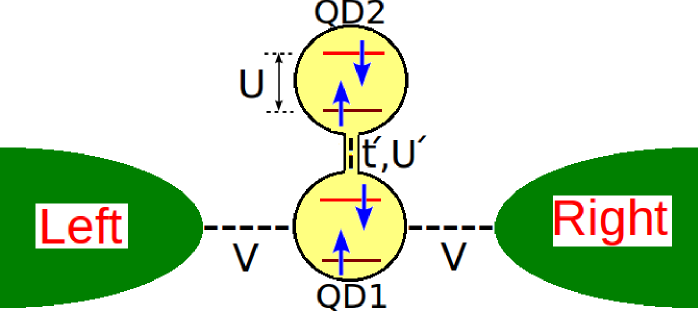
Figure 1: (color online) Schematic representation of the DQD system being analyzed in this work. Note the capacitive interaction, $U^{\prime}$, between the dots.

II Theoretical model and numerical methods

We study a system composed by two QDs (from now on referred to as QD1 and QD2) coupled by a tunneling matrix element as well as by capacitive inter-dot Coulomb repulsion. This system is described by the generalized Anderson Hamiltonian, which can be written as

$$H=H_{imp}+H_{cb}+H_{hyb},$$ (1)

where $H_{imp}$ is the Hamiltonian describing the QDs [which we define as “impurity region”], $H_{cb}$ describes the conduction bands, and $H_{hyb}$ describes the coupling of QD1 and the conduction bands (see Fig. 1). More explicitly,

$$H_{imp} = \sum_{i=1,2\atop\sigma}\varepsilon_{i}c^{\dagger}_{i\sigma}c_{i\sigma}+\sum_{i=1,2}U_{i}n_{i\uparrow}n_{i\downarrow}+U^{\prime}n_{1}n_{2}$$ (2)

$$+t^{\prime}\sum_{\sigma}\left[c^{\dagger}_{1\sigma}c_{2\sigma}+c^{\dagger}_{2\sigma}c_{1\sigma}\right],$$

where the operator $c^{\dagger}_{i\sigma}$ ($c_{i\sigma}$) creates (annihilates) an electron in the $i$-th ($i=1,2$) QD, with energy $\varepsilon_{i}$, spin $\sigma$, $n_{i\sigma}=c^{\dagger}_{i\sigma}c_{i\sigma}$ is the number operator, and $n_{i}=\sum_{\sigma}n_{i\sigma}$. The second term in $H_{imp}$ corresponds to the on-site Coulomb repulsion, where, for simplicity we will take the intra-dot interactions $U_{1}=U_{2}=U$ throughout this paper. The third term describes the inter-dot Coulomb repulsion $U^{\prime}$ due to the proximity of the dots, and the last term describes the coupling between the two dots, with tunneling matrix element $t^{\prime}$.

$$H_{cb}=\sum_{\ell k\sigma}\varepsilon_{\ell k}c^{\dagger}_{\ell k\sigma}c_{\ell k\sigma},$$ (3)

where the operator $c^{\dagger}_{\ell k\sigma}$ ($c_{\ell k\sigma}$) creates (annihilates) an electron with momentum $k$, energy $\varepsilon_{\ell k}$, and spin $\sigma$ in the $\ell$-th lead ($\ell=L,R$). Finally,

$$H_{hyb}=\sum_{k\sigma}\left[V_{\ell k}c^{\dagger}_{1\sigma}c_{\ell k\sigma}+V_{\ell k}^{*}c^{\dagger}_{\ell k\sigma}c_{1\sigma}\right].$$ (4)

Notice that QD2 couples to the band indirectly through QD1.

For simplicity, we assume the hybridization coupling $V_{\ell k}=V$ to be real, independent of $k$, and the same for both leads. The conduction band is characterized by a constant density of states given by $\rho_{c}(\omega)=\Theta(D-|\omega|)/2D$, where $D$ is the half-bandwidth and $\Theta(x)$ is the standard Heaviside step function. To properly study the low-temperature physics of this setup we employ Wilson’s NRGWilson (1975); Krishna-murthy et al. (1980a, b) approach, which allows for a systematic assessment of the Kondo effect in impurity systems. Within the NRG, we logarithmically discretize the conduction band and map it into a tridiagonal form, which corresponds to a semi-infinite chain where the coupling between the sites has the form

$$t_{N}=\frac{(1+\Lambda^{-1})(1-\Lambda^{-N-1})}{2\sqrt{1-\Lambda^{-2N-1}}\sqrt{1-\Lambda^{-2N-3}}}~{}\Lambda^{-N/2},$$ (5)

where $\Lambda$ is the discretization parameter (all results shown here are for $\Lambda=2.5$). The “impurity” site ($N-1$) possesses sixteen degrees of freedom, corresponding to all the base-states necessary to fully describe the quantum state of the two QDs, while the other $N\geq 0$ sites correspond to single non-interacting sites of Wilson’s chain. Denoting the base-states of $H_{-1}=H_{imp}$ for the QDs as

$$\mid\phi_{i}\rangle_{-1}\equiv\mid m_{1},m_{2}\rangle_{-1}$$ (6)

where $m_{k}=1,2,3,4$ corresponds respectively to $0,\uparrow,\downarrow$ or $\uparrow\downarrow$. In this basis the Hamiltonian $H_{-1}$ has matrix elements

$$[H_{-1}]_{ij}=_{-1}\hskip-2.84544pt\langle\phi_{i}\mid H_{-1}\mid\phi_{j}\rangle_{-1}.$$ (7)

By diagonalizing the matrix defined in Eq. 7 we obtain a set of sixteen eigenstates $\mid\Psi_{i}\rangle_{-1}$ with corresponding eigenenergies $E_{i}^{(-1)}$. In terms of the base-states the eigenstates can be written as

$$\mid\Psi_{i}\rangle_{-1}=\sum_{j}A_{ij}\mid\phi_{j}\rangle_{-1},$$ (8)

where $A_{ij}$ is the projection of the $i$-th eigenvector onto the $j$-th base-state. Once we obtain the eigenstates, we calculate all the necessary matrix elements for the next iteration, after which we add a new site $N=0$. To describe the resulting system we enlarge the Hilbert space such that the new basis is constructed performing all 64 possible combinations

$$\mid\phi_{i}\rangle_{0}:=\mid m\rangle\otimes\mid\Psi_{j}\rangle_{-1},$$ (9)

where $m=1,\cdots,4$ and $j=1,\cdots,16$. This procedure is repeated until the system has reached its strong-coupling fix point. When the dimension of the Hilbert space becomes larger than $N_{s}$, where typically $N_{s}=2500$, it is truncated by discarding the eigenstates corresponding to the largest eigenenergies. At each iteration $N$ we keep the energy spectrum $E^{(N)}_{i}$, together with the matrix elements necessary to calculate the relevant physical quantities. This procedure allows us to calculate thermodynamical properties, such as entropy $S$, magnetic moment $\mu^{2}=k_{B}T\chi_{imp}$, spin-spin correlation $\langle\textbf{S}_{1}\cdot\textbf{S}_{2}\rangle$, occupation numbers $n_{i\sigma}\equiv\langle n_{i\sigma}\rangle$, etc, as well as dynamical quantities, like density of states (DOS) and conductance. For the entropy and magnetic moment it is usual to define the contribution from the impurity as $S_{imp}$ and $\mu^{2}_{imp}$. These quantities are generically written as $X_{imp}=X-X_{0}$, where $X_{0}$ is calculated in the absence of the impurity. Within the canonical ensemble, as a function of temperature $T_{N}$, we can write,

$$X(T_{N})=\frac{1}{Z_{N}(T_{N})}\sum_{i}{{{}_{N}}}\langle\Psi_{i}\mid\hat{X}\mid\Psi_{i}\rangle_{N}e^{-\beta_{N}E^{(N)}_{i}},$$ (10)

where $\beta_{N}=(T_{N})^{-1}$, and

$$T_{N}=\frac{1}{2k_{B}\bar{\beta}}D(1+\Lambda^{-1})\Lambda^{-(N-1)/2}$$ (11)

is a characteristic temperature associated to the $N$-th iteration, $\bar{\beta}$ is a real number of order 1, $\hat{X}$ is the operator associated to the quantity $X$ and

$$Z_{N}(T_{N})=\sum_{i}e^{-\beta_{N}E^{(N)}_{i}}$$ (12)

is the canonical partition function.

The conductance is calculated by the generalized Landauer formula

$$G/G_{0}=-\sum_{\sigma}\int_{-\infty}^{\infty}{\tt Im}[{\cal T}_{\sigma}(\omega)]\left[\partial f(\omega)/\partial\omega\right]d\omega,$$ (13)

where ${\cal T}_{\sigma}(\omega)=2\pi V^{2}\rho_{c}(\omega)G_{11}^{\sigma}(\omega)$, $G_{0}=(2e^{2}/h)$ and $G_{11}(\omega)$ is the Fourier transform of the full interacting double-time Green’s function

$$G^{\sigma}_{ii}(t,t^{\prime})=-i\Theta(t-t^{\prime})\Big{\langle}\left[c_{i\sigma}(t),c^{\dagger}_{i\sigma}(t^{\prime})\right]\Big{\rangle},$$ (14)

which in the present case results to be spin independent. The Green’s function is calculated at frequency $\omega_{N}=D(1+\Lambda^{-1})\Lambda^{-(N-1)/2}$ within NRG in a standard manner via Lehmann representation,

$$G^{\sigma}_{ii}(\omega_{N}) = \sum_{nn^{\prime}}\frac{\mid{{{}_{N}}}\langle\Psi_{n}\mid c_{i\sigma}\mid\Psi_{n^{\prime}}\rangle_{N}\mid^{2}}{\omega_{N}-\left(E^{(N)}_{n}-E^{(N)}_{n^{\prime}}\right)}$$ (15)

$$\times\left(e^{-\beta E^{(N)}_{n}}+e^{-\beta E^{(N)}_{n^{\prime}}}\right).$$

We also employ a logarithmic Gaussian broadeningBulla et al. (2001) of the discrete NRG spectrum in order to obtain a smooth curve for the QDs DOS at arbitrary frequency $\omega$

$$\rho^{\sigma}_{i}(\omega)=-\frac{1}{\pi}{\tt Im}G^{\sigma}_{ii}(\omega),$$ (16)

necessary to calculate the conductance at finite temperature.

III Numerical results

In order to proceed with our numerical analysis, let us set $D$, typically the largest energy scale of the problem, as our energy unit ($D=1$). We then choose for all calculations $U_{1}=U_{2}=U=5\times 10^{-4}$ and $V=3.2\times 10^{-3}$, so that $U/\pi\Gamma_{1}\approx 5$, where $\Gamma_{1}=2\pi V^{2}\rho_{0}$, and $\rho_{0}=1/(2D)$. We will study in detail the two cases where $U^{\prime}=0$ and $U^{\prime}=U$, and also the range $0<U/U^{\prime}<1$ The bare levels $\varepsilon_{1}$ and $\varepsilon_{2}$ will be controlled by the same gate voltage ($V_{g}$), such that $\varepsilon_{1}=\varepsilon_{2}=V_{g}$. With the parameters set above, and $V_{g}=-U/2$ (i.e., with the system at the particle-hole (p-h) symmetric point), we can estimate the Kondo temperature for the single QD asKrishna-murthy et al. (1980a) $T_{K}=\sqrt{\Gamma_{1}U}\exp(-\pi U/8\Gamma_{1})\approx 2.89\times 10^{-7}$ for QD1, when QD2 is completely disconnected ($t^{\prime}=0$ and $U^{\prime}=0$).

III.1 $U^{\prime}=0$ case

Although this case has been studied in great detail in Ref. Cornaglia and Grempel, 2005, we will present below some results that will help us understand the more complicated situation at finite $U^{\prime}$. In Figs. 2 and 3, we show results for the temperature dependence of the entropy and the square of the total magnetic moment of the DQD system, $S_{imp}/k_{B}\ln(2)$ and $\mu^{2}_{imp}/(g\mu_{B})^{2}$, for $U^{\prime}=0$, $\varepsilon_{1}=\varepsilon_{2}=-U/2$ and various values of $t^{\prime}$, where $k_{B}$ is Boltzmann’s constant and $\mu_{B}$ is the Bohr magneton. For the special case where $t^{\prime}=0$ [(black) ○curve], the DQD corresponds to the case where just QD1 is coupled to the conduction band and QD2 is completely decoupled from the rest of the system. In this situation, as the temperature decreases, we find the following regimes: (i) for $k_{B}T\sim D\gg U$ the DQD is in its free orbital (FO) regime; in this regime, the temperature is high enough to allow for all the sixteen DQD states to be populated. This results in an entropy $S_{imp}=k_{B}\ln(16)$ (see Fig. 2) and a total square magnetic moment $\mu^{2}=2\times(g\mu_{B})^{2}/8$ (Fig. 3), (ii) for $k_{B}T_{K}<k_{B}T<\varepsilon_{1},\varepsilon_{2}$, thermally excited charge fluctuations are suppressed, and therefore the entropy decreases to $S_{imp}=k_{B}\ln(4)$, as only states with one electron in each QD are favored. This implies that $\mu^{2}$ increases, as double and unoccupied states in each QD are suppressed, and the DQD is in the so-called local moment (LM) regime. As the temperature decreases further, and becomes lower than $T_{K}$, QD2 remains in its LM regime, while the other spin is progressively screened by the conduction electrons due to the formation of the Kondo state, with the electrons in the leads screening the spin of QD1. This regime is characterized by the plateaus $S_{imp}=k_{B}\ln(2)$ and $\mu^{2}_{imp}=(g\mu_{B})^{2}/4$. These contributions arise just from the spin in QD2, as it is never Kondo screened when $t^{\prime}=0$.

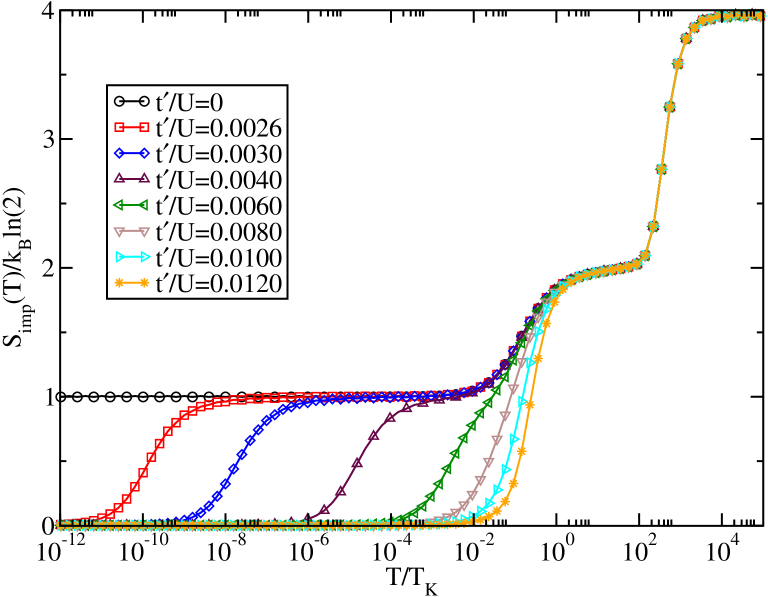
Figure 2: (color online) Temperature variation of the entropy for various values of $t^{\prime}$ (see legend). The other parameters are $U_{1}=U_{2}=5\times 10^{-4}$, $U^{\prime}=0$, $\varepsilon_{1}=\varepsilon_{2}=-2.5\times 10^{-4}$, and $V=3.2\times 10^{-3}$. Note that the temperature in the horizontal axis is scaled by the Kondo temperature of QD1 (see text), which, for the parameters chosen, is $T_{K}=2.89\times 10^{-7}$. Details for the different regimes are provided in the text.

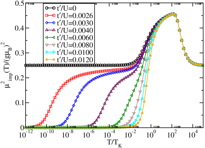
Figure 3: (color online) Magnetic moment $k_{B}T\chi$ as function of temperature for various values of $t^{\prime}$. All parameters are the same as in Fig. 2.

For finite $t^{\prime}$, however, the behavior of the DQD for temperatures below $T_{K}$ is quite different from the one just discussed above for $t^{\prime}=0$. For very small values of $t^{\prime}$, as shown in Ref. Cornaglia and Grempel, 2005, the DQD system presents a TSK effect, where $both$ QD1 and QD2 spins are screened by the conduction band, but the screening of the spin in QD2 occurs at a much lower temperature than that at which the spin in QD1 is screened. The second screening stage emerges at a characteristic temperature $T_{K}^{\prime}$ which depends mainly upon $t^{\prime}$ and $T_{K}$ (the Kondo temperature for QD1) as

$$T_{K}^{\prime}=aT_{K}\exp{(-bT_{K}/J^{\prime})},$$ (17)

where $a$ and $b$ are real positive numbers, with values approximately 1, and $J^{\prime}=4t^{\prime 2}/U$ is an effective antiferromagnetic coupling (between electrons in QD1 and QD2) favoring a local singlet state that competes with the regular Kondo energy scale $T_{K}$. As a result, a TSK effect is expected for $J^{\prime}<T_{K}$. We can clearly see this behavior, for example, when $t^{\prime}/U=0.0030$ [(blue) $\Diamond$ curve] in Figs. 2 and 3. Note that for this value of $t^{\prime}/U$ the second drop in the entropy (signaling the screening of the electron in QD2) happens at $T_{K}^{\prime}\approx 10^{-17}$, with $J^{\prime}\approx 1.35\times 10^{-8}$ (for this value of $t^{\prime}$) being much larger than $T_{K}^{\prime}$ (remember that $T_{K}\sim 2.89~{}10^{-7}$. As $t^{\prime}$ increases, and eventually $J^{\prime}$ becomes larger than $T_{K}$, a strong singlet is formed locally, destroying the TSK picture. A detailed discussion of this crossover can be found in Ref. Cornaglia and Grempel, 2005, here, instead, we focus on the effect of the inter-dot Coulomb repulsion, as discussed in the next section.

III.2 Finite $U^{\prime}$

III.2.1 Entropy and magnetic moment

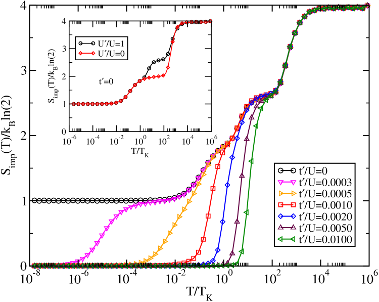
Figure 4: (color online) Same as in Fig. 2, but now for $U^{\prime}=U$ and different values of $t^{\prime}$ (see legend). The Kondo temperature used to scale the horizontal axis is that obtained for $U^{\prime}=U$ and $t^{\prime}=0$. The inset contains a comparison of $t^{\prime}=0$ results between $U^{\prime}=0$ [(black) $\Circle$ curve] and $U^{\prime}=U$ [(red) $\Diamond$ curve], showing that the Kondo temperature of the first stage (for $t^{\prime}=0$) does not depend on $U^{\prime}$.

Now, we turn on $U^{\prime}$ and for simplicity we choose $U^{\prime}=U$ (later on, we will analyze results for $0<U^{\prime}<U$). The new features to note in the entropy (in relation to the results in Fig. 2, for $U^{\prime}=0$) are (i) the very clear plateau (in Fig. 2) at $S_{imp}/k_{B}\ln(2)=2$ splits into two narrower plateaus in Fig. 4: one at $S_{imp}/k_{B}\ln(2)\approx 2.66$, and the one at $S_{imp}/k_{B}\ln(2)=2$ becomes less well defined, more like a shoulder. The plateau at $\approx\ln(6)/\ln(2)=2.58$ (starting at $T\approx 10^{2}~{}T_{K}$) comes from the fact that now, as $U^{\prime}=U$, all 6 states with 2 electrons have very similar energies. As the temperature goes further down, the 4 states that can participate in a Kondo state in QD1 (one electron in each QD) will have lower energy and the shoulder around $S_{imp}/k_{B}\ln(2)=2$ will form (at $T\approx T_{K}$), (ii) to obtain the second stage of the TSK (signaled by a plateau at $S_{imp}/k_{B}\ln(2)=1$, for finite $t^{\prime}$) one needs to go to one order of magnitude smaller values of $t^{\prime}$, when compared to the results for $U^{\prime}=0$ (compare the (purple) $\triangle$ curve in Fig. 2, for $t^{\prime}=0.004$, with the (purple) $\triangle$ curve in Fig. 4, for $t^{\prime}=0.005$, where all traces of the second stage in the TSK effect have vanished), (iii) it is also apparent that, contrary to the $U^{\prime}=0$ case, $T^{\prime}_{K}$ depends much more strongly on $t^{\prime}$. Indeed, it is clear that the temperature at which the entropy starts to decrease to zero becomes considerably higher as $t^{\prime}$ increases, conversely to what can be seen in Fig. 2. It is important to note that the horizontal axis in Fig. 4 is scaled by the Kondo temperature (for QD1) for $t^{\prime}=0$, estimated with the expression in the text above. In the inset to Fig. 4 we show that $T_{K}$ for $U^{\prime}=0$ and $U^{\prime}=U$ are equal. Indeed, as illustrated by the agreement between the entropy curves (for $T<T_{K}$) calculated with $t^{\prime}=0$ [(black) $\Circle$ curve for $U^{\prime}=U$, and (red) $\Diamond$ curve for $U^{\prime}=0$].

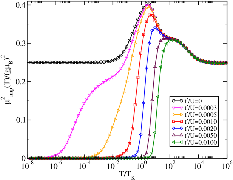
Figure 5: (color online) Magnetic moment $k_{B}T\chi$ as function of temperature for various values of $t^{\prime}$. All parameters are the same as in Fig. 4.

In relation to the magnetic susceptibility, a few differences are quite apparent when $U^{\prime}$ is turned on: (i) for the three smallest values of $t^{\prime}$, in Fig. 5, the peak in the susceptibility has moved down to $\approx T_{K}$, and the maximum value of the magnetic moment is now lower ($0.4$ for finite $U^{\prime}$, as compared to $\approx 0.45$ for $U^{\prime}=0$). The decrease in the magnetic moment comes from the two extra states (two electrons in each dot) that are now part of this manifold of states, and which have zero magnetic moment; (ii) as $t^{\prime}$ increases, the peak moves up in temperature (up to $T=10^{2}~{}T_{K}$) and the maximum value of the magnetic moment further decreases, down to $\mu^{2}_{imp}/(g\mu_{B})^{2}\approx 0.3$ for $t^{\prime}=0.01$, (iii) for the three smaller values of $t^{\prime}$, the splitting of the single plateau in the magnetic moment translates into a higher temperature shoulder (around $T/T_{K}=10^{2}$), which is not present for $U^{\prime}=0$. This shoulder becomes also the maximum value of the magnetic moment for $t^{\prime}=0.01$ (the largest $t^{\prime}$ results calculated).

However, the most important differences coming from adding $U^{\prime}$ are related to the behavior of $T_{K}$ and $T_{K}^{\prime}$. First, the value of $T_{K}$ being used for the scaling of the horizontal axis is that obtained when $t^{\prime}=0$. Note from Figs. 2 and 3, that $T_{K}$ is very weakly dependent on $t^{\prime}$ when $U^{\prime}=0$. That is clearly not the case for $U^{\prime}=U$, where it can be seen a strong variation of $T_{K}$ and $T_{K}^{\prime}$ with $t^{\prime}$. In addition, more interestingly from an experimental point of view, it is clear that the ratio $T_{K}^{\prime}/T_{K}$ increases by a few orders of magnitude for $U^{\prime}=U$.

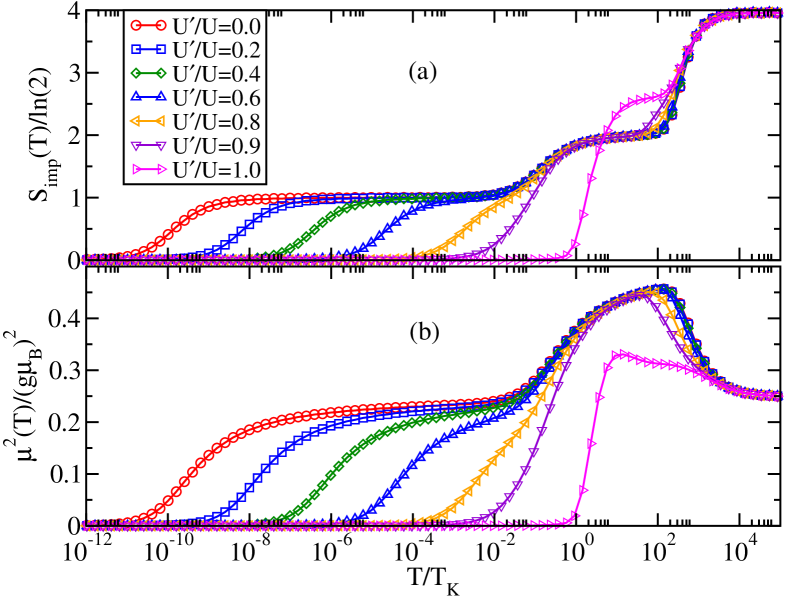
Figure 6: (color online) (a) Entropy $S_{imp}$ and (b) Magnetic moment $k_{B}T\chi$ as function of temperature for various ratios of $U^{\prime}/U$ (between 0 and 1, see legend) for $t^{\prime}/U=0.0026$. To preserve the p-h symmetry for each curve we set $V_{g}=-U/2+U^{\prime}$. All the other parameters are the same as in Figs. 4 and 5. It is clear from the results that the Kondo temperature for the second stage of the TSK effect is greatly enhanced (by a few orders of magnitude) when $U^{\prime}$ increases.

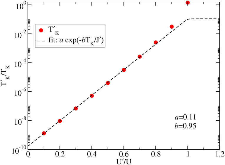
Figure 7: (color online) Fitting (dashed line) of the $T_{K}^{\prime}$ values [red dots] extracted from Fig. 6, obtained by using eqs. 17 and 18. The values obtained (from the fitting) for the two free parameters a and b are indicated in the figure.

To analyze in more detail the increase of $T_{K}^{\prime}$ with $U^{\prime}$ we show, in Fig. 6, results for entropy [panel (a)] and magnetic moment [panel (b)] which clearly indicate the strong increase in $T_{K}^{\prime}$ (by a few orders of magnitude) when the ratio $U^{\prime}/U$ varies from 0 to 1 for a fixed value of $t^{\prime}/U=0.0026$. This increase in $T_{K}^{\prime}$ can be understood by estimating the Kondo temperature $T_{K}^{\prime}$ for the second stage of the TSK, by using eq. 17, and explicitly calculating $J^{\prime}$ for finite $U^{\prime}$:

$$J^{\prime}=-\frac{U-U^{\prime}-\sqrt{(U-U^{\prime})^{2}+16t^{\prime 2}}}{2},$$ (18)

indicating that, at least for small values of $U^{\prime}/U$ (where $J^{\prime}\sim 4t^{\prime 2}/(U-U^{\prime})$, there should be an exponential increase of $T_{K}^{\prime}$ with $U^{\prime}/U$. This expectation is supported by the NRG results shown in Fig. 6. One can go one step further and, substitute eq. 18 into eq. 17, and use the equation thus obtained to fit the values of $T_{K}^{\prime}$ that can be extracted from Fig. 6. This fitting is shown in Fig. 7. Note that the only free parameters in the fitting shown in Fig. 18 are ‘a’ and ‘b’ (values indicated in the figure). It can be clearly seen that fitting (at least up to $U^{\prime}/U\sim 0.7$ is very good (note that the vertical axis is in a logarithmic scale). Indeed, this is one of the principal results of this paper. Given the recent advances in the use of floating interdot capacitors (see Ref. Chan et al., 2002), values of $U^{\prime}/U$ for double dot systems have been steadily increasing, and may, in light of our results, offer the hope of observing the so far experimentally inaccessible energy scale $T_{K}^{\prime}$.

III.2.2 Zero-temperature case: QD occupation and conductance

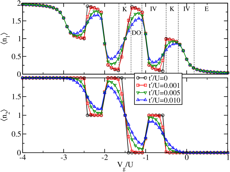
Figure 8: (color online) Total occupation $\langle n_{1}\rangle$ (top) and $\langle n_{2}\rangle$ (bottom) as function of gate voltage ($V_{g}$) for $t^{\prime}/U=0$ ($\Circle$), $t^{\prime}/U=1.0\times 10^{-3}$ ($\square$), $t^{\prime}/U=2\times 10^{-3}$ ($\Diamond$) and $t^{\prime}/U=1.0\times 10^{-2}$ (${\triangle}$). Other parameters are $t^{\prime}/U=5\times 10^{-4}$ and $V=3.2\times 10^{-3}$. The regions delimited by the vertical lines refer to QD1 states, namely, empty (E), intermediate valence (IV), Kondo (K) and doubly occupied (DO) intermediate valence.

We first study how the occupation of the dots, $\langle n_{i}\rangle\equiv\sum_{\sigma}\langle n_{i\sigma}\rangle$, is modified due to inter-dot Coulomb repulsion. In Fig. 8, we show $\langle n_{1}\rangle$ (top) and $\langle n_{2}\rangle$ (bottom) as function of $V_{g}$ for various values of $t^{\prime}$. For $t^{\prime}=0$ [(black) $\Circle$ curve], as $V_{g}\approx 0$ one can observe a smooth increase of $\langle n_{1}\rangle$, while $\langle n_{2}\rangle$ remains zero all the way down to $V_{g}/U\approx-0.5$, where $\langle n_{2}\rangle$ jumps to $1$ and $\langle n_{1}\rangle$ abruptly decreases. The discontinuous increase of $\langle n_{2}\rangle$ is due to the sharp peak in the local density of states (LDOS) $\rho_{2}$ of level $\epsilon_{2}$, which is not broadened for $t^{\prime}=0$. On the other hand, $\langle n_{1}\rangle$ increases smoothly, as $\epsilon_{1}$ is broadened by $\Gamma_{1}$. The value of $V_{g}$ for which the first discontinuity of $\langle n_{2}\rangle$ occurs (expected to be at $V_{g}\approx 0$, when $U^{\prime}=0$) depends on the additional capacitive energy necessary to put electrons in different dots, due to the inter-dot Coulomb repulsion $U^{\prime}$.

As discussed by three of the current authors in a previous work,Büsser et al. (2011) this gate-voltage-dependent charge oscillation can be understood as a competition between the Kondo and Intermediate Valence (IV) regimes: level $\epsilon_{2}$, when $t^{\prime}=0$, acts as a dark state, whose charge occupation, which can only be an integer, adds a step function of height $U^{\prime}$ to the gate potential $V_{g}$ in QD1 (depending on $\langle n_{2}\rangle$ being 0 or 1). The value of $V_{g}$ for which the transition of $\langle n_{2}\rangle$ between 0 and 1 (and vice versa) occurs depends on $\Gamma_{1}$ and reflects which many-body regime, Kondo or IV, better optimizes the energy of QD1. The dark state $\varepsilon_{2}$ acts like a switch between the two regimes and may have applications in quantum computation.Pemberton-Ross et al. (2010); Büsser et al. (2011) For example, when the first discontinuity occurs, for $V_{g}/U\approx-0.5$, QD1 is in a Kondo state, however, further decrease of $V_{g}$ makes it more favorable for QD1 to be in an IV state, which can be accomplished by charging QD2 (by exactly one electron), this, due to the capacitive coupling, increases the effective gate potential of QD1, discharging it, and bringing it back to the IV regime. As $V_{g}/U$ further decreases below $-0.5$, QD1 starts to transition from an IV to a Kondo state; when $V_{g}/U\approx-1$, again the IV state for QD1 is more favorable; this regime can now be achieved by completely avoiding the Kondo regime through the discontinuous charging of QD1 by one extra electron. Total charge is kept constant by discharging QD2 completely ($\langle n_{2}\rangle=0$). Finally, further decrease of $V_{g}$, bringing it close to the p-h symmetric point [$V_{g}=-(U/2+U^{\prime})=-3U/2$], increases the charge in QD1 to almost 2 electrons; at this point, the Kondo state in QD1 is more favorable, and a new discharging and charging occurs of QD1 and QD2, respectively, after which, each QD hosts one electron. These gate-voltage-dependent occupancy oscillations are clearly observed for all curves in Fig. 8, with the difference that, for finite $t^{\prime}$, there are no discontinuities. Indeed, for finite $t^{\prime}$, discontinuities in the $\langle n_{i}\rangle$ are no longer observed, we rather notice that the jumps are smoothened out as $t^{\prime}$ increases. This continuous charging of QD2 now results from the broadening $\Gamma_{2}$ of the local bare (and also the many-body) level at QD2. For the non-interacting case it is easily shown that $\Gamma_{2}\propto t^{\prime 2}\Gamma_{1}$. It is important to note the differences and similarities between this model and the one studied in Ref. Büsser et al., 2011: in the latter, one has a two channel system, where the dark state, for small values of $t_{-}$, acquires a finite broadening and smoothen out the discontinuities seen in the $\langle n_{1}\rangle$ and $\langle n_{2}\rangle$ curves in Fig. 8. In the model being studied here, a similar process occurs: the dark state in QD2 acquires a broadening through its connection $t^{\prime}$ to the single conduction channel through QD1. Nonetheless, through a comparison of Fig. 8 in this work with Fig. 4 in Ref. Büsser et al., 2011 [panels (c) and (d)], one can see that qualitatively the results are very similar, indicating that the basic processes determining the gate voltage dependent occupancy oscillations are the same.

The strong gate-dependent variations in $\langle n_{i}\rangle$ ($i=1,~{}2$) (caused by the capacitive coupling) are expected to have dramatic influence in the conductance of the system, specially in the Kondo regime. For $U^{\prime}=0$, and in the special case where $t^{\prime}=0$, QD1 will be in a Kondo state for all $V_{g}$ values in the interval $[-U,0]$. For finite $U^{\prime}$, however, the charging and discharging of the QDs moves QD1 from a Kondo to an IV regime, and vice versa. For the case of $t^{\prime}=0$ [(black) $\Circle$ curve in Fig. 9], when $V_{g}$ becomes negative, we observe a narrow Kondo plateau of height $G_{0}$, and then the conductance drops suddenly to almost zero at $V_{g}/U\approx-0.5$, which is exactly the gate potential value where QD1 is discharged (see Fig. 8). This drop signals the transitioning of QD1 from the Kondo to the IV regime, as described above and in Ref. Büsser et al., 2011. The small peak (of height $0.3~{}G_{0}$) observed at $V_{g}/U\approx-1$ corresponds to the discontinuous jump of the renormalized level $\tilde{\epsilon}_{1}\approx\varepsilon_{1}+U^{\prime}\langle n_{2}\rangle$, caused by the discontinuous change in $\langle n_{2}\rangle$ from $1$ to $0$, leading QD1 from a low occupancy ($\langle n_{1}\rangle\approx 0.0$) IV regime, to a high ($\langle n_{1}\rangle\approx 2.0$) IV regime, completely skipping the Kondo regime (with occupancy $\langle n_{1}\rangle\approx 1.0$).

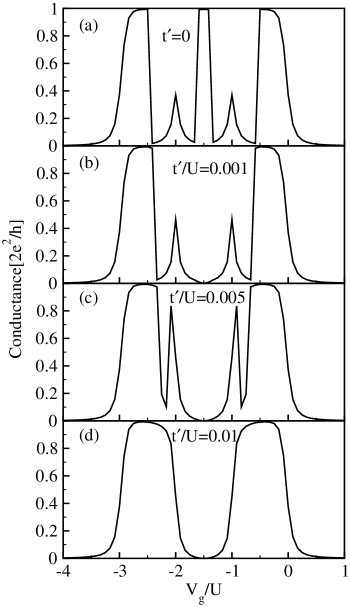
Figure 9: (color online) Zero-temperature conductance as a function of $V_{g}$ for the same parameters as in Fig. 8. The occupancy discontinuities analyzed in Fig. 8 are associated to the discontinuities seen here for the conductance. See text for a full description of the variation of the peak structures with increasing $t^{\prime}$: (a) $t^{\prime}/U=0$, (b) $t^{\prime}/U=10^{-3}$, (c) $t^{\prime}/U=5\times 10^{-3}$, and (d) $t^{\prime}/U=10^{-2}$.

When the system reaches the vicinity of its p-h symmetric point [$V_{g}=-(U/2+U^{\prime})=-3U/2$], there are exactly two electrons in the QDs (one in each) and the Kondo effect is fully reestablished in QD1 (for $t^{\prime}=0$), thus the conductance reaches $G_{0}$. Due to p-h symmetry, the other half of the curve can be explained in a similar way. The (black) $\Circle$ curve in Fig. 9 should be compared to the right-side panel of Fig. 3(b) in Ref. Büsser et al., 2011.

For increasing $t^{\prime}$ there are mainly two differences in the charge and in the conductance: i) the abruptness of the charging/discharging and the discontinuities in the conductance are progressively smoothed out, and ii) the central peak in the conductance (around the p-h symmetric point) is fully suppressed. For example, for $t^{\prime}/U=1\times 10^{-3}$, a rapid drop in the QD occupations is still clearly visible (as observed on the $\square$ (red) curve in Fig. 8), resulting in a rapid variation in the conductance, which now moves down to a lower value of $V_{g}$ when compared with the $t^{\prime}=0$ curve (see $\square$ curve in Fig. 9). Notice that the peak at $V_{g}\approx-U$ is enhanced, as $t^{\prime}$ increases, as now the value of $V_{g}$ in the IV regime corresponds to a higher conductance. For even larger $t^{\prime}$ there is a continuous enhancement of the conductance as $V_{g}$ approaches $-U$, as clearly observed for $t^{\prime}/U=1.0\times 10^{-2}$. The suppression of the conductance around the p-h symmetric point for small (but finite) $t^{\prime}$ results from destructive Fano-like interference due to the Kondo resonance in QD2. For large $t^{\prime}$, on the other hand, results from the formation of a local singlet due to an antiferromagnetic effective coupling ($J=4t^{\prime 2}/U$) between the two electrons in the QDs, competing with the Kondo singlet formed between the electron in QD1 and the conduction electrons. This is clearly associated to the TSK effect previously analyzed in this system. Cornaglia and Grempel (2005)

One should note that there is a striking difference in the effect of $t^{\prime}$ over the conductance for different regions of gate potential, and for different values of $t^{\prime}$. For the smallest value studied ($t^{\prime}$), as mentioned above, the Kondo peak at half-filling is immediately suppressed and this can be associated to the TSK effect. On the other hand, the peak around $V_{g}=-U$ is barely affected for a small $t^{\prime}$. Indeed, as the TSK effect depends on the energy scale $J^{\prime}$, one expects that it will be more effective at half-filling. Higher values of $t^{\prime}$ will then quickly modify the structures around $V_{g}=-U/2$: the peak at $V_{g}=-U$ is quickly enhanced and shifted to higher gate voltage values, while the discontinuity located (for $t^{\prime}=0$) at $V_{g}=-U/2$ moves to lower gate potential values, extending the Kondo plateau, until the two structures merge and form a single Kondo peak centered at $V_{g}=-U/2$. This occurs because now level $\epsilon_{2}$ acquires a finite width and therefore the discharging of QD1 (and simultaneous charging of QD2) is not abrupt anymore and the system smoothly proceeds from the IV to the Kondo regime.

III.2.3 Finite-temperature case

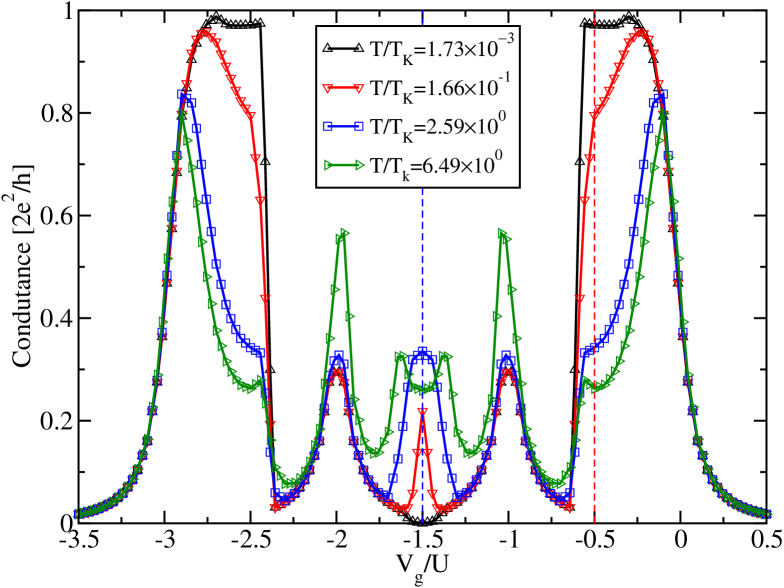
Figure 10: (color online) Conductance as function of $V_{g}$ for $U_{2}=U_{1}$, $t^{\prime}/U=1.0\times 10^{-3}$ for $T/T_{K}=7.31\times 10^{-10}$ ($\Circle$), $T/T_{K}=1.08\times 10^{-4}$ ($\square$), $T/T_{K}=1.70\times 10^{-3}$ ($\Diamond$), $T/T_{K}=1.66\times 10^{-1}$ ($\triangle$), $T/T_{K}=6.49\times 10^{0}$ ($\triangleright$).

Now we turn our attention to the effect of temperature in the transport properties of the system described in Fig. 1. In Fig. 10, we show the conductance for $U^{\prime}=U$, $t^{\prime}/U=1.0\times 10^{-3}$, and various values of temperature. The curves in this figure should be compared to the corresponding zero temperature curves in Fig. 9 [(red) $\square$ curve]. Starting with $T/T_{K}=1.7\times 10^{-3}$ [(black) $\bigtriangleup$] we notice a very similar shape when compared to the $T=0$ results [(red) $\square$] in Fig. 9, except that the two symmetric Kondo plateaus and the IV peaks at $V_{g}/U\approx-1$ and $V_{g}/U\approx-2$ are slightly suppressed, which results from the small (but finite) temperature. Results for smaller temperatures (not shown) interpolate between $T=0$ and $T/T_{K}=1.7\times 10^{-3}$. For $T/T_{K}=1.66\times 10^{-1}$ [(red) $\triangledown$] we observe a clear suppression of the Kondo plateau while, the IV peaks do not differ much from those for lower temperatures. This is readily understood since the characteristic energy of the Kondo state $T_{K}$ is much smaller than the energy scale associated to the IV regime, of order $\Gamma_{1}$ (for details, see Fig. 8 in Ref. Büsser et al., 2011). On the other hand, it is interesting to notice the emergence of a sharp small peak at the p-h symmetric point for a higher temperature such as $T/T_{K}=1.66\times 10^{-1}$ [(red) $\triangledown$]. This peak results from a revival of the Kondo peak observed for $t^{\prime}=0$ in the $T=0$ case, see the corresponding curve in Fig. 9 [(black) $\Circle$]. This revival of the Kondo peak results from the progressive restoration of the Kondo singlet state in QD1 as the local singlet is suppressed when $T^{\prime}_{K}<T<T_{K}$. For $T>T_{K}$, as in the (green) $\triangleright$ curve, we observe a suppression of the p-h Kondo peak, similar to a splitting.

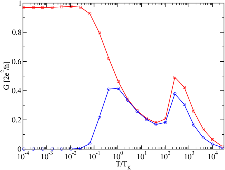
Figure 11: (color online) Conductance as function of temperature for $t^{\prime}/U=1.0\times 10^{-3}$ for $V_{g}/U=-1.5$ [(blue) $\Circle$] and $V_{g}=-0.5$ [(red) $\square$], along the (blue and red) dashed vertical lines shown in Fig. 10.

In order to show this effect in more detail, in Fig 11 we plot the temperature variation of the conductance for the same parameters as in Fig. 10, for two different values of $V_{g}$. For $V_{g}/U=-1.5$ [(blue) $\Circle$ curve], the conductance vanishes when $T\rightarrow 0$, increases for $10^{-2}\lesssim T/T_{K}\lesssim 10^{-1}$, and is suppressed again for $T\gtrsim T_{K}$. Note that the initial enhancement of the conductance as the temperature increases results from the destruction of the Kondo resonance in the QD2, suppressing the destructive interference between the two paths. Conversely, as the temperature keeps increasing, and $T$ exceeds $T_{K}$, the conductance is suppressed due to the destruction of the Kondo resonance in QD1. Finally, it will rise again and reach a maximum at approximately $T/T_{K}\sim 10^{2}\approx\Gamma_{1}$ due to charge fluctuations in QD1. For $V_{g}=-0.5$ [(red) $\square$ curve], i.e., at the edge of the right plateau of Fig. 10], the conductance starts from $G_{0}=2e^{2}/h$ as $T\rightarrow 0$, and is suppressed for $10^{-2}~{}T_{K}\lesssim T\lesssim 10~{}T_{K}$ due to the destruction of the Kondo effect in QD1. This is the behavior of the regular Kondo effect in a single QD. It is interesting to point out that once the temperature is above $T^{\prime}_{K}$, the conductance at both $V_{g}$ values behave alike.

In Fig. 12, similarly to Fig. 10, we show $G~{}vs.~{}V_{g}$, for different temperatures, but now for $t^{\prime}=1\times 10^{-2}$, the largest $t^{\prime}$ value used in Fig. 9. These curves should be compared to the zero-temperature (blue) $\triangle$ curve in Fig. 9. For the case of $T/T_{K}\sim 10^{-10}$, the curve has the same shape as the corresponding curve in Fig. 9. We notice, however, that by gradually increasing the temperature, both Kondo plateaus become valleys surrounded by two Coulomb blockade peaks, while the gap at the p-h symmetric point remains almost unchanged. This is in consistent with what one would expect of the charge transport at high temperature for two molecular levels.

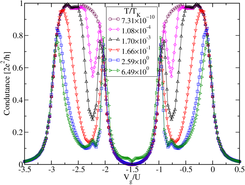
Figure 12: (color online) Conductance as function of $V_{g}$ and $t^{\prime}/U=0.01$ for various temperatures in the $U_{2}=U_{1}$, $t^{\prime}/U=1.0\times 10^{-2}$ and $T/T_{K}=7.31\times 10^{-10}$ ($\Circle$), $T/T_{K}=1.08\times 10^{-4}$ ($\Diamond$), $T/T_{K}=1.70\times 10^{-3}$ ($\triangle$), $T/T_{K}=1.66\times 10^{-1}$ ($\triangledown$), $T/T_{K}=2.59\times 10^{0}$ ($\square$), and $T/T_{K}=6.49\times 10^{0}$ ($\triangleright$).

IV Concluding remarks

We have studied a strongly interacting double dot system arranged in a T-shape configuration, where the dots are coupled via a tunneling matrix element and also strong inter-dot Coulomb repulsion. We have presented a detailed study of the effect of the inter-dot Coulomb interaction on the Kondo physics of the system. Our numerical analysis reveals interesting crossovers between different mixed valence and Kondo regimes that produce dramatic changes in the conductance of the system. These crossovers can be tuned by varying the gate voltage of the QDs, and the charging/discharging processes produce anomalous peaks in the conductance across the system, allowing a clear identification of the various regimes. We show that the inter-dot Coulomb repulsion not only preserves the TSK regime, but it also dramatically increases the lowest energy scale of the TSK effect. Indeed, $T_{K}^{\prime}$ increases exponentially with the inter-dot Coulomb interaction, as shown in panels 9a) and (b) of Fig. 6. We stress that this enhancement may allow the experimental observation of this so far elusive effect. Finally, by fixing the gate voltage at the p-h symmetric point and raising the temperature, the conductance shows clearly the crossover from TSK to Kondo and then to mixed valence regime (see Fig. 11). By contrast, away from the p-h symmetry only the regular Kondo regime is observed. For temperatures larger than $T_{K}$ (and large enough values of the coupling $t^{\prime}$ between the QDs) the conductance of the system as a function of the gate voltage possesses a four-peak structure, showing clearly the Coulomb blockade regime of the molecular orbitals of the system. Finally, we believe that our results will motivate future experimental measurements.