11email: dgruber@mpe.mpg.de 22institutetext: Green Cross Capital Pty Ltd, 495 Harris St, Ultimo, NSW 2007, Australia 33institutetext: Institute of Astro and Particle Physics, University Innsbruck, Technikerstrasse 25, 6176 Innsbruck, Austria 44institutetext: University of Alabama in Huntsville, NSSTC, 320 Sparkman Drive, Huntsville, AL 35805, USA 55institutetext: Los Alamos National Laboratory, P.O. Box 1663, Los Alamos, NM 87545, USA 66institutetext: Universities Space Research Association, NSSTC, 320 Sparkman Drive, Huntsville, AL 35805, USA 77institutetext: Space Science Office, VP62, NASA/Marshall Space Flight Center Huntsville, AL 35812, USA
Quasi-Periodic Pulsations in Solar Flares:
new clues from the Fermi Gamma-Ray Burst Monitor
Abstract
Aims. In the last four decades it has been observed that solar flares show quasi-periodic pulsations (QPPs) from the lowest, i.e. radio, to the highest, i.e. gamma-ray, part of the electromagnetic spectrum. To this day, it is still unclear which mechanism creates such QPPs. In this paper, we analyze four bright solar flares which show compelling signatures of quasi-periodic behavior and were observed with the Gamma-Ray Burst Monitor (GBM) onboard the Fermi satellite. Because GBM covers over 3 decades in energy (8 keV to 40 MeV) it can be a key instrument to understand the physical processes which drive solar flares.
Methods. We tested for periodicity in the time series of the solar flares observed by GBM by applying a classical periodogram analysis. However, contrary to previous authors, we did not detrend the raw light curve before creating the power spectral density spectrum (PSD). To assess the significance of the frequencies we made use of a method which is commonly applied for X-ray binaries and Seyfert galaxies. This technique takes into account the underlying continuum of the PSD which for all of these sources has a dependence and is typically labeled red-noise.
Results. We checked the reliability of this technique by applying it to a solar flare which was observed by the Reuven Ramaty High-Energy Solar Spectroscopic Imager (RHESSI) which contains, besides any potential periodicity from the Sun, a 4 s rotational period due to the rotation of the spacecraft around its axis. While we do not find an intrinsic solar quasi-periodic pulsation we do reproduce the instrumental periodicity. Moreover, with the method adopted here, we do not detect significant QPPs in the four bright solar flares observed by GBM. We stress that for the purpose of such kind of analyses it is of uttermost importance to appropriately account for the red-noise component in the PSD of these astrophysical sources.
Key Words.:
Sun: flares, Methods: data analysis, Methods: statistical, Methods: observational1 Introduction
Over the last 40 years quasi-periodic pulsations (QPP) in solar flares have been reported from observations across the electromagnetic spectrum, i.e. from radio waves up to the high energetic gamma-rays ranging from sub-second timescales up to several minutes (e.g. Parks & Winckler 1969; Ofman & Sui 2006; Li & Gan 2008; Nakariakov & Melnikov 2009; Nakariakov et al. 2010a). While there seems to be an overwhelming amount of observational data, the underlying physical mechanism which could generate such QPPs remains still a mystery. Possible processes that are considered are modulation of electron dynamics by magnetohydrodynamic (MHD) oscillations (Zaitsev & Stepanov 1982), periodic triggering of energy releases by MHD waves (Foullon et al. 2005; Nakariakov et al. 2006), MHD flow overstabilities (Ofman & Sui 2006) and oscillatory regimes of magnetic reconnection (Kliem et al. 2000).
In this paper we will present time series and periodogram analyses of four solar flares which show an intriguing quasi-periodic behavior in their light curves. All of these solar flares were observed by the Fermi Gamma-Ray Burst Monitor (GBM, Meegan et al. 2009). GBM is one of the instruments onboard the Fermi Gamma-Ray Space Telescope (Atwood et al. 2009) launched on June 11, 2008. Specifically designed for gamma-ray burst (GRB) studies, GBM observes the whole unocculted sky with a total of 12 thallium-activated sodium iodide (NaI(Tl)) scintillation detectors covering the energy range from 8 keV to 1 MeV and two bismuth germanate scintillation detectors (BGO) sensitive to energies between 150 keV and 40 MeV (Meegan et al. 2009). Therefore, GBM offers superb capabilities for the analyses of not only GRBs but solar flares as well.
The analysis and interpretation of power spectral density (PSD) of solar flares is, in general, difficult. A variety of astrophysical sources (such as X-ray binaries, Seyfert galaxies (e.g. Lawrence et al. 1987; Markowitz et al. 2003) and GRBs (Ukwatta et al. 2009; Cenko et al. 2010)), show erratic, aperiodic brightness changes. Solar flares exhibit similar aperiodic variations with the general time profile being a sharp impulsive phase followed by a slower decay phase. Solar flares, together with many other astrophysical sources, thus have very steep power spectra in the low-frequency region. This type of variability is known as red-noise (e.g. Groth 1975; Deeter & Boynton 1982; Vaughan 2005). When determining the significance of possible periodicities in the PSD the red-noise has to be accounted for in order not to severely overestimate the significance of identified frequencies (Lachowicz et al. 2009). In this paper we will account for the red-noise properties when performing a periodogram analysis.
This paper is organized as follows. In Sect.2 we briefly present the methodology of the time-series analysis. We provide an overview of the red-noise properties in astrophysical sources and demonstrate the importance of the red-noise when estimating significances. In Sect.3 we will present light curves and periodograms of solar flares which were observed by GBM. Finally, in Sect.4, we will summarize and conclude.
2 Analysis of data governed by red-noise
As it was already pointed out by Mandelbrot & Wallis (1969) and Press (1978), the human eye has a tendency to identify periodicities from purely random time series, i.e. where sinusoidal variations are not statistically real. According to Press (1978) the strongest eye-apparent period in (actually non-periodic) data will be about one-third the length of the data sample. According to these authors “three-cycle” quasiperiods should be taken with a grain of salt.
Solar flares fall into the group of astrophysical sources where red-noise is important. Red-noise has nothing to do with measurement errors or systematics of the detectors, which are also called noise. Red-noise is an intrinsic property of the observed source and is due to erratic, aperiodic brightness changes. Contrary to white noise, which displays a flat spectrum in a PSD, i.e. is power independent of frequency, red-noise is characterized by a power law of the form of . As a first order approximation, red-noise is the realization of a linear stochastic and weakly non-stationary process. This red-noise component makes the interpretation of the significance of a peak in the PSD more complex.
One way to estimate the significance of induced frequencies on top of an underlying red-noise continuum in a PSD, was presented by Vaughan (2005).
In short, Vaughan suggests to calculate the periodogram normalized so that the units of power are (e.g. Schuster 1898; Press & Rybicki 1989). Then, the periodogram is converted to log-space in both frequency and power. For such a log-periodogram one can than clearly identify the power-law component in the low-frequency range and a “cutoff” where white noise or an additional noise component takes over (e.g. Ukwatta et al. 2009). One can easily determine the power-law parameters by fitting a linear function to the low-frequency periodogram bins using the least-squares method. In this paper the method of Vaughan (2005) was slightly modified in that we use a broken power law (BPL) to fit the PSD instead of a single power law.
2.1 Red-noise simulation
It is common practice (Inglis et al. 2008; Nakariakov et al. 2010a) to suppress the low-frequency component by de-trending the light curves of solar flares. This can be achieved by smoothing the light curve with a moving average or by applying a Gaussian filter and perform the periodogram analysis on the residual emission, i.e. the smoothed version is subtracted from the original data-set. This can give rise to misleading results as we will show in the following.

By randomizing the phase as well as the amplitudes, Timmer & Koenig (1995) introduced an algorithm to generate a purely random time series which shows a dependence in the PSD. We created a time series consisting of 300 data points, evenly spaced by 1 s with a periodogram shape. From this light curve, we subtracted a simple moving average of 50 s (see Fig. 1). We then calculated the PSD (first described by Lomb (1976) and Scargle (1982)) and then refined by Press & Rybicki 1989) on the residuals. The result is striking. Although we started with a purely random, red-noise dominated time-series we obtain a PSD with three frequencies whose power exceeds the confidence limit (calculated according to Scargle 1982). This approach in signal processing clearly returns false-positive frequencies with periods of s, s and s, respectively. When the periodogram is calculated over the original light curve, using the Vaughan (2005) approach, i.e. with a single power law fit to the data, the spectral peaks remain below the threshold.
Therefore, by this example, we strongly discourage subtracting smoothed versions of raw light curves when looking for intrinsic frequencies in the red-noise dominated PSD.
2.2 Detour: QPPs in GRBs
The same procedure of light curve reprocessing with a subsequent PSD analysis has also been applied for GRBs. These events are the most luminous flashes of -rays known to mankind, believed to originate from highly relativistic outflows from a compact source with Lorentz factors . In 2009, the Swift-BAT satellite (Gehrels et al. 2004) observed GRB 090709A (Morris et al. 2009). Soon after the detection, Markwardt et al. (2009) claimed to have found a very unusual behavior, not observed in any other GRB so far, namely a QPP like behavior with a periodicity of s at the 12 level of significance. This QPP was subsequently confirmed and found to be in phase in the data of the Anticoincidence System (ACS) of the spectrometer SPI on board the INTEGRAL satellite (Götz et al. 2009), the Konus-WIND instrument (Golenetskii et al. 2009) and the Suzaku Wide-band All-sky Monitor (WAM) (Ohno et al. 2009). These latter instruments operate in the energy ranges 80 keV-10 MeV, 20 keV-1150 keV and 50 keV-5 MeV, respectively. Swift-BAT, on the other hand, is sensitive in the energy range 15 keV-150 keV.
However, soon thereafter, Cenko et al. (2010) showed that the interpretation of this QPP strongly depends on the assumption of the underlying continuum. If, in fact, it is accounted for, the significance of the claimed periodicity drops below the 3 confidence limit. This analysis was independently repeated by Iwakiri et al. (2010) and de Luca et al. (2010) who also took into account the red-noise component in the PSD, and only find a marginally significant periodicity at the confidence limit.
In conclusion to this detour, we emphasize once more the importance to account for the red-noise component in the PSD. Additionally, we draw attention to the fact that a potential quasi-periodic signal is not necessarily significant even if it is identified in several instruments with different (but overlapping) energy ranges and observed to be in phase across these bands.
2.3 Method testing
The Reuven Ramaty High-Energy Solar Spectroscopic Imager (RHESSI, Lin et al. 2002) rotates around its spin axis which is always pointed towards the Sun. The period of this rotation is s and a PSD analysis of the RHESSI light curves is expected to display this instrumental signal. We applied the Vaughan (2005) test to a solar flare which has been observed by RHESSI on January 1st, 2005 and where QPPs have been reported (Nakariakov et al. 2010a). This solar flare peaked at 00:31 UT at a GOES level X1.7, from the NOAA active region 10715 located on disk at N03E47. We used RHESSI data in the energy range from 50 keV-100 keV with a fine time resolution of 0.1 s (see upper panel of Fig.2) and performed two periodogram analyses on this light curve in the range between 1660 s and 1820 s. The first periodogram analysis was performed using the classical approach introduced by Lomb (1976) and Scargle (1982). Similarly to what has been commonly done in the past (e.g. Inglis & Nakariakov 2009) a periodogram has been calculated on the residual emission after a simple moving average of 50 s has been subtracted from the raw data (see middle panel of Fig.2). With this method, several peaks are found above the 3 threshold. The peak with the highest value of normalized power is located at Hz, corresponding to the periodicity reported by Nakariakov et al. (2010a). Another peak which is worth mentioning is located at Hz which is the expected rotational frequency of RHESSI around its spin axis.


As we will show in the following, the significance of the peak at Hz is highly overestimated by the latter method. We show a PSD which was calculated using the raw and undetrended light curve applying the technique by Vaughan (2005) in the bottom panel of Fig.2. Analogically to the Lomb and Scargle periodogram analysis, we found a significant spectral feature at Hz which is the expected rotation period of the RHESSI instrument. However, this PSD is lacking any other frequency above the 3 confidence limit. The discrepancy between the two methods is easily explained. Firstly, the whole raw light curve was used without artificially detrending it beforehand. Secondly, the method by Lomb and Scargle assumes a white noise continuum and does not take into consideration the red noise component of the solar flare. However, the latter is taken into account by the method of Vaughan. In conclusion, we could not confirm the reported QPP in this solar flare. We are confident that this latter method can be used for further analysis since we believe that it is more adequate for sources which are dominated by red-noise and the inherent rotational frequency of the instrument is found to be significant.

An additional check was performed using SPI-ACS data of the outburst of the soft gamma repeater SGR 1806-20 observed on December 27th, 2004 in the energy range from 80 keV to 8 MeV (Mereghetti et al. 2005). SGR 1806-20 is known to have a rotational period of 7.56 s and the methodology adopted here should be able to recover this periodicity. We removed the very bright initial pulse and focused on the emission from s to 175 s (see Fig.3). We unambiguously recover the main pulsation period ( s) together with the first, second, third and fifth harmonic.
We conclude that the here applied methodology is appropriate and reliable for the further analysis.
3 Solar flares observed by GBM
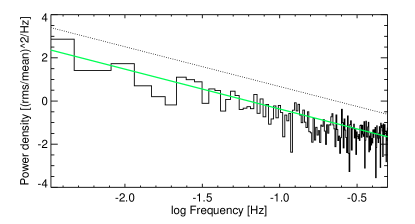
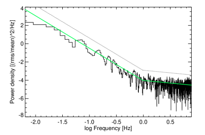
3.1 Solar flare on February 24, 2011 at 07:29:20.71 UT
For the purpose of its analysis we use CSPEC and CTIME data of detectors NaI 3, NaI 4 and NaI 5 with a time-resolution of 1.024 s (4.096 s pre-trigger) and 0.064 s (0.256 s pre-trigger), respectively. In the energy range from 50 keV to 1 MeV this solar flare lasted for about 500 s. The light curve (Fig.4) consists of several peaks and a compellingly looking quasi-periodic behavior lasting to s. After de-trending the raw light curve with a simple moving average (50 s) the QPP pattern becomes more visible (see inset of Fig.4). Applying a standard periodogram analysis (Lomb 1976; Scargle 1982) on the detrended light curve several peaks are above the confidence limit as can be seen in the middle panel of Fig.4.


However, applying the previously introduced method (Vaughan 2005) on the original light curve, thus taking into account the red-noise properties of the source we did not find any significant QPP during the solar flare life-time, as is pointed out in the lower panel of Fig.4. We performed this analysis making use of the CTIME data with a time resolution of 64 ms. The PSD has been calculated for the signal spanning from () s to ( s), where denotes the time of trigger.
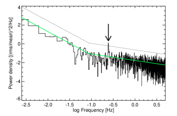
3.2 Solar flare on June 12, 2010 at 00:55:05 UT
For the analysis we use again CSPEC and CTIME data of detectors NaI 0 through NaI 5. The count rate is not increasing significantly for the first 30 s in the 50 keV to 1 MeV energy range. After this time there is a sharp increase in the flare brightness which then decays again very rapidly after 60 s. The whole duration of the solar flare in this energy range is approximately 120 s. Overlaid on top of the observed light curve, again one can identify a compellingly looking QPP behavior with a period of s (see upper panel of Fig.5). This periodicity is apparently significant when applying a standard Lomb-Scargle periodogram (see middle panel of Fig.5) on the detrended light curve. The smoothing length was 15 s.


However, the PSD, computed for CTIME data with a time resolution of 64 ms in the interval () s to () s and according to Vaughan (2005), does not show a significant periodicity.
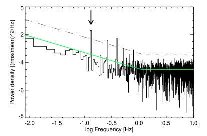
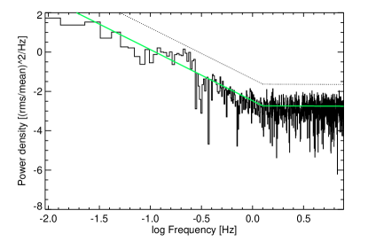
3.3 Solar flare on March 15, 2011 at 00:21:15.69 UT
For the analysis we use again CTIME data of detectors NaI 0 through NaI 5 in an energy range covering 50 keV to 1 MeV with a time resolution of 0.256 s. The total duration of the solar flare in this energy range is approximately 50 s (see Fig.6). For the Lomb-Scargle periodogram analysis (see middle panel of Fig.6) the light curve was detrended with a simple moving average of 5 s. Repeating the PSD analysis on the original data set between () s and () s according to Vaughan (2005) we did not find any significant QPP.


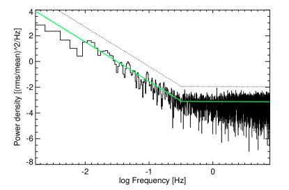
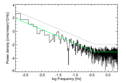
3.4 Solar flare on March 14, 2011 at 19:50:17.3 UT
For the analysis we use the same data type, energy range and time resolution as for solar flare #4 in Sect.3.3. The total duration of the solar flare is approximately 150 s (see Fig.7). Contrary to the a Lomb-Scargle periodogram which finds a significant periodicity in the detrended light curve (smoothing length of 10 s), the PSD, determined in the time interval between () s and () s and done according to Vaughan (2005), does not find any significant QPP.


4 Summary & Conclusions
We have analyzed light curves of five solar flares observed by both GBM and RHESSI. We tested the data for the presence and significance of QPPs accounting for the overall shape of the PSD by applying the method introduced by Vaughan (2005). First of all, this technique was validated and tested by applying it on raw data of the RHESSI satellite. Any RHESSI light curve has an inherent period caused by the rotation of the space craft around its axis. With the method adopted here we successfully retrieve this well known 4 s period. However, we were not able to confirm the previously reported QPP of 40 s in the very same solar flare (Nakariakov et al. 2010a). An additional check was performed by applying the method to SPI-ACS data of the giant flare of the well known SGR 1806-20. This magnetar has a rotation period of s which, together with several harmonics, could be recovered unambiguously with the procedure presented here. These two tests gave us confidence that the method is appropriate to test the significance of QPPs in red-noise dominated solar flare time series.
The routine was then applied to four solar flares observed by GBM. Although all of these solar flares showed very promising quasi-periodic features in their detrended light curves at first none of these were significant ( 3 ). Previous authors (e.g. Inglis et al. 2008; Inglis & Nakariakov 2009; Zimovets & Struminsky 2010; Nakariakov et al. 2010a) who claim a significant QPP detection, applied a standard Lomb-Scargle analysis to detrended solar flare light curves. Our investigation of this method suggests the power in the low frequency range is being artificially suppressed, which can lead to misleading values for the significances of features in the PSD. A periodogram analysis should always be performed on the raw and undetrended light curve as was done here.
We stress once more that not only solar flares but many astrophysical sources (X-ray binaries, Seyfert galaxies, GRBs) suffer from steep power spectra in the low-frequency range. Such power spectra make a periodogram analysis not trivial, the interpretation of a peak in a PSD more complex and an estimation of its significance an important issue. Again we emphasize that red-noise is an intrinsic source property. In other words, having shown that the variations in the corresponding solar flares are not quasi-periodic at the 3 level does not mean that these variations are not real. The corresponding flux changes are sometimes dramatic, reaching a factor of a few within a few tens of seconds. Also, these variations occur in phase at different X-ray to gamma-ray energies, and other flares have been observed to also occur in phase with microwave radio emission (e.g. Nakariakov et al. 2010a; Foullon et al. 2010).
References
- Atwood et al. (2009) Atwood, W. B., Abdo, A. A., Ackermann, M., et al. 2009, ApJ, 697, 1071
- Cenko et al. (2010) Cenko, S. B., Butler, N. R., Ofek, E. O., et al. 2010, AJ, 140, 224
- de Luca et al. (2010) de Luca, A., Esposito, P., Israel, G. L., et al. 2010, MNRAS, 402, 1870
- Deeter & Boynton (1982) Deeter, J. E. & Boynton, P. E. 1982, ApJ, 261, 337
- Foullon et al. (2010) Foullon, C., Fletcher, L., Hannah, I. G., et al. 2010, ApJ, 719, 151
- Foullon et al. (2005) Foullon, C., Verwichte, E., Nakariakov, V. M., & Fletcher, L. 2005, A&A, 440, L59
- Gehrels et al. (2004) Gehrels, N., Chincarini, G., Giommi, P., et al. 2004, ApJ, 611, 1005
- Golenetskii et al. (2009) Golenetskii, S., Aptekar, R., Mazets, E., et al. 2009, GRB Coordinates Network, 9647, 1
- Götz et al. (2009) Götz, D., Mereghetti, S., von Kienlin, A., & Beck, M. 2009, GRB Coordinates Network, 9649, 1
- Groth (1975) Groth, E. J. 1975, ApJS, 29, 453
- Inglis & Nakariakov (2009) Inglis, A. R. & Nakariakov, V. M. 2009, A&A, 493, 259
- Inglis et al. (2008) Inglis, A. R., Nakariakov, V. M., & Melnikov, V. F. 2008, A&A, 487, 1147
- Iwakiri et al. (2010) Iwakiri, W., Ohno, M., Kamae, T., et al. 2010, in American Institute of Physics Conference Series, Vol. 1279, American Institute of Physics Conference Series, ed. N. Kawai & S. Nagataki, 89–92
- Kliem et al. (2000) Kliem, B., Karlický, M., & Benz, A. O. 2000, A&A, 360, 715
- Lachowicz et al. (2009) Lachowicz, P., Gupta, A. C., Gaur, H., & Wiita, P. J. 2009, A&A, 506, L17
- Lawrence et al. (1987) Lawrence, A., Watson, M. G., Pounds, K. A., & Elvis, M. 1987, Nature, 325, 694
- Li & Gan (2008) Li, Y. P. & Gan, W. Q. 2008, Sol. Phys., 247, 77
- Lin et al. (2002) Lin, R. P., Dennis, B. R., Hurford, G. J., et al. 2002, Sol. Phys., 210, 3
- Lomb (1976) Lomb, N. R. 1976, Ap&SS, 39, 447
- Mandelbrot & Wallis (1969) Mandelbrot, B. B. & Wallis, J. R. 1969, Water Resources Research 5, 1, 228
- Markowitz et al. (2003) Markowitz, A., Edelson, R., Vaughan, S., et al. 2003, ApJ, 593, 96
- Markwardt et al. (2009) Markwardt, C. B., Gavriil, F. P., Palmer, D. M., Baumgartner, W. H., & Barthelmy, S. D. 2009, GRB Coordinates Network, 9645, 1
- Meegan et al. (2009) Meegan, C., Lichti, G., Bhat, P. N., et al. 2009, ApJ, 702, 791
- Mereghetti et al. (2005) Mereghetti, S., Götz, D., von Kienlin, A., et al. 2005, ApJ, 624, L105
- Morris et al. (2009) Morris, D. C., Beardmore, A. P., Evans, P. A., et al. 2009, GRB Coordinates Network, 9625, 1
- Nakariakov et al. (2010a) Nakariakov, V. M., Foullon, C., Myagkova, I. N., & Inglis, A. R. 2010a, ApJ, 708, L47
- Nakariakov et al. (2006) Nakariakov, V. M., Foullon, C., Verwichte, E., & Young, N. P. 2006, A&A, 452, 343
- Nakariakov et al. (2010b) Nakariakov, V. M., Inglis, A. R., Zimovets, I. V., et al. 2010b, Plasma Physics and Controlled Fusion, 52, 124009
- Nakariakov & Melnikov (2009) Nakariakov, V. M. & Melnikov, V. F. 2009, Space Science Reviews, 149, 119
- Ofman & Sui (2006) Ofman, L. & Sui, L. 2006, ApJ, 644, L149
- Ohno et al. (2009) Ohno, M., Iwakiri, W., Suzuki, M., et al. 2009, GRB Coordinates Network, 9653, 1
- Parks & Winckler (1969) Parks, G. K. & Winckler, J. R. 1969, ApJ, 155, L117+
- Press (1978) Press, W. H. 1978, Comments on Astrophysics, 7, 103
- Press & Rybicki (1989) Press, W. H. & Rybicki, G. B. 1989, ApJ, 338, 277
- Reznikova & Shibasaki (2011) Reznikova, V. E. & Shibasaki, K. 2011, A&A, 525, A112+
- Scargle (1982) Scargle, J. D. 1982, ApJ, 263, 835
- Schuster (1898) Schuster, A. 1898, Journal of Geophysical Research, 3, 13
- Timmer & Koenig (1995) Timmer, J. & Koenig, M. 1995, A&A, 300, 707
- Ukwatta et al. (2009) Ukwatta, T. N., Dhuga, K. S., Parke, W. C., et al. 2009, ArXiv e-prints
- Vaughan (2005) Vaughan, S. 2005, A&A, 431, 391
- Zaitsev & Stepanov (1982) Zaitsev, V. V. & Stepanov, A. V. 1982, Soviet Astronomy Letters, 8, 132
- Zimovets & Struminsky (2010) Zimovets, I. V. & Struminsky, A. B. 2010, Sol. Phys., 263, 163