Noncommutative $\kappa$-Minkowski $\phi^{4}$ theory:
Construction, properties and propagation

Abstract:

Noncommutative (NC) $\kappa$-deformation of a spacetime, whose NC coordinates close in a Lie algebra, affects the coalgebra of the Poincaré group and the algebra of physical fields. This leads to a modification of the multiplication in the corresponding universal enveloping algebra. The usual pointwise multiplication has to be replaced by a deformed star product. The measure problems in the $\kappa$-Minkowski spacetime are avoided because the measure function is naturally absorbed in the new ${\star}_{h}$-product. That reflects itself in the way we have constructed the deformed NC scalar $\phi^{4}$ action. The action is further modified by adding a harmonic oscillator term and expanding up to linear order in the deformation parameter $a$. This leads to an effective theory on commutative spacetime. Furthermore, we obtain modified equations of motion and conserved currents. In order to compute the tadpole contributions to the scalar field propagation/self-energy, we anticipate that statistics on $\kappa$-Minkowski spacetime is specifically deformed. Thus, our prescription in fact corresponds to a hybrid approach of standard quantum field theory (QFT) and NCQFT on $\kappa$-deformed Minkowski spacetime. The results are analyzed in the framework of the two-point Green’s function for low, intermediate and Planckian energies, respectively. For low energies $E$, the dependence of the tadpole contribution on the $\kappa$-deformation parameter $a$ completely drops out. At Planckian propagation energies, it tends to a finite fixed value, which only depends on the Planckian energy and/or the $\kappa$-deformation parameter. Semiclassical/hybrid behavior of the first order quantum effects do show up due to the $\kappa$-deformed momentum conservation law. The mass term of the scalar field is shifted and these shifts are dramatically different at different propagation energies. At Planckian energies, the $\kappa$-modified dispersion relations show the genuine effect of birefringence. We conclude that our results could have physical consequences e.g. in the NC Higgs sector and the connection to quantum gravity.

1 Introduction

Two basic areas of interest, namely quantum gravity and the deformation of the Poincaré algebra, make $\kappa$-Minkowski spacetime to an important subject of theoretical investigations from both, physical as well as mathematical perspective.

An argument in favor of $\kappa$-Minkowski spacetime is the indication that it could arise in the context of quantum gravity coupled to matter fields [1, 2]. These considerations show that after integrating out the gravitational topological degrees of freedom of gravity, the effective dynamics of matter fields is described by a noncommutative quantum field theory which has a $\kappa$-Poincaré group as its symmetry [3, 4, 5]. In this context, the $\kappa$-Minkowski spacetime can be, and there are some arguments to support this, considered as a flat limit of quantum gravity.

Second, $\kappa$-Minkowski spacetime emerges naturally from the $\kappa$-Poincaré algebra [6, 7, 8, 9, 10], which provides a possible group theoretical framework for the describing of the so-called Doubly Special Relativity (DSR) theories [11, 12, 13, 14, 15, 16]. Although different proposals for DSR theories can be considered as different bases [15, 16] for the $\kappa$-Poincaré algebra, they all represent the same noncommutative structure. This situation makes noncommutative field theories on noncommutative $\kappa$-Minkowski spacetime an even more interesting subject to study. Various attempts have been undertaken in this direction by many authors [17, 18, 19, 20, 21, 22, 23].

Recently, it was established that $\kappa$-Minkowski spacetime leads to modification of the particle statistics described by deformed oscillator algebras [24, 25, 26, 27, 28, 29, 30]. Deformation quantization of Poincaré algebra can be performed by means of the twist operator [31, 32, 33, 34, 35] which happens to include the dilatation generator. Thus, the twist belongs is an element of the universal enveloping algebra of the general linear algebra [36, 37, 38, 39, 40]. It also gives rise to a deformed statistics on $\kappa$-Minkowski spacetime [25, 37, 41, 42]. However, since the $\kappa$-Poincaré Hopf algebra is a quantum symmetry described only approximatively by the twisted quantum algebra, identifying charges and conserved current and therefore also establishing a Noether theorem could be problematic. A certain modification of momentum conservation is necessary in order to obtain a reasonable physics out of the twisted Hopf algebra prescription of our theory.

The transition from the $\kappa$-deformed to the commutative Minkowski spacetime in the case of the free fields was described in [43], while the star product and interacting fields were treated in the same approach in [44]. The problem of UV/IR mixing and $\kappa$-deformation was discussed in [45]. In correspondence to the above observations, as well as by comparing the deformed dispersion relations to the corresponding time delay calculations of high energy photons, bounds can be put on the deformation (quantum gravity) scale [46, 47, 48]. In the present work, we are work with commutative Minkowski spacetime endowed with a $\kappa$-deformed star product. The considered $\kappa$-deformed symmetry of the Minkowski spacetime has an undeformed Lorentz sector (classical basis [49, 15, 16, 50]) and its noncommutative coordinates close in the $\kappa$-deformed Lie algebra and additionally, form a Lie algebra together with the Lorentz generators [51, 52, 53, 54]. This deformation of the spacetime structure affects the algebra of physical fields, leading to a modification of the multiplication in the corresponding universal enveloping algebra. As mentioned before, the usual pointwise multiplication has to be replaced by a deformed star product, i.e. by the new star product ${\star}_{h}$. This star product together with the usual integration enjoys the important trace property [54]. The integral measure problems for $\kappa$-Minkowski spacetime are avoided, since the measure function is naturally absorbed in the new ${\star}_{h}$-product. The action is further modified by adding a harmonic oscillator term [55, 56] and expanding up to first order in the deformation parameter $a$. The resulting action should be considered as an effective theory on commutative spacetime. Furthermore, we obtain modified equations of motion and conserved currents to first order in $a$. Next, in order to compute the tadpole contributions to the scalar field propagation/self-energy, we anticipate that statistics on $\kappa$-Minkowski spacetime is specifically deformed. Expanding the model was necessary in order to be able to compute relevant physical quantities, such as the self-energy of the complex scalar field $\phi$. The above properties are very welcome, however, we have to stress that by truncating the $\kappa$-deformed action at the linear order in the deformation parameter $a$ we have lost nonperturbative quantum effects like the celebrated UV/IR mixing [45], which, for example, connects NC field theories to Holography via UV and IR cutoffs in a model independent way [57, 58]. Resummation of the expanded action can in principle restore the nonperturbative character of the theory, see e.g. [60, 61, 62]. Those are general properties of most of the NCQFT expanded/resummed in terms of the noncommutative deformation parameter. Holography and UV/IR mixing are possible windows to quantum gravity [57, 58, 59].

In the same line of reasoning, we should take into account the harmonic oscillator term, despite that it is well known that such a term breaks translational invariance [55, 56]. Our approach generally represents a hybrid approach of standard quantum field theory and NCQFT on $\kappa$-Minkowski spacetime, including $\kappa$-deformed momentum conservation law [17, 19, 20, 63, 64].

In a next step, we discuss the results in the framework of two-point Green’s function for low, intermediate and the Planck scale energy regime, respectively. We have found semiclassical behavior of the first order quantum effects, and, as a consequence, a shift of the mass term of the scalar field. This shift depends on the energy. Thus, the dispersion relations are $\kappa$-deformed and we have found a genuine birefringence effects, [65, 66] of the massive scalar field mode at first order in the deformation parameter $a$. This is similar to the fermion field birefringence in truncated Moyal $\star$-product theories [66].

Above, we have described the main results of this paper, which could be of physical importance for example for the $\kappa$-deformed scalar field (Higgs) and its propagation, as well as to quantum gravity.

In the first section, we give some mathematical preliminaries including the Hopf algebra structure of $\kappa$-deformed Minkowski spacetime and star products. In the second section, we introduce, the hermitian realization and the corresponding star product $\star_{h}$. The modified $\kappa$-deformed scalar field action based on the above notions is introduced next, and the equations of motion are derived. The corresponding currents are conserved. The properties of our new $\kappa$-deformed action on ordinary Minkowski spacetime are discussed in the last section. This includes $\kappa$-deformed Feynman rules and the field propagation via computation of two-point Green’s function within the proposed model.

2 Mathematical preliminaries of $\kappa$-deformed Minkowski spacetime

2.1 Hopf algebra and star product

We are considering a $\kappa$-deformation of the Minkowski spacetime whose symmetry has an undeformed Lorentz sector and whose noncommutative coordinates $\hat{x}_{\mu},~{}(\mu=0,1,...,n-1),$ close in a Lie algebra together with the Lorentz generators $M_{\mu\nu},~{}(M_{\mu\nu}=-M_{\nu\mu})$  :

$$[\hat{x}_{\mu},\hat{x}_{\nu}] =i(a_{\mu}\hat{x}_{\nu}-a_{\nu}\hat{x}_{\mu})\,,$$ (2.1)

$$[M_{\mu\nu},M_{\lambda\rho}] =\eta_{\nu\lambda}M_{\mu\rho}-\eta_{\mu\lambda}M_{\nu\rho}-\eta_{\nu\rho}M_{\mu\lambda}+\eta_{\mu\rho}M_{\nu\lambda}\,,$$ (2.2)

$$[M_{\mu\nu},\hat{x}_{\lambda}] =\hat{x}_{\mu}\eta_{\nu\lambda}-\hat{x}_{\nu}\eta_{\mu\lambda}-i\left(a_{\mu}M_{\nu\lambda}-a_{\nu}M_{\mu\lambda}\right)\,,$$ (2.3)

where the deformation parameter $a_{\mu}$ is a constant Lorentz vector and $~{}\eta_{\mu\nu}=diag(-1,1,\cdot\cdot\cdot,1)$ defines the metric in this spacetime. The quantity $a^{2}=a_{\mu}a^{\mu}$ is Lorentz invariant having a dimension of inverse mass squared, $a^{2}\equiv\frac{1}{{\kappa}^{2}}.$ The above algebra satisfies all the Jacobi identities and therefore forms a Lie algebra with the property that in the limit $a_{\mu}\rightarrow 0,$ the commutative spacetime with the usual action of the Lorentz algebra is recovered. Throughout the paper we will work in natural units, $\hbar=c=1$.

The symmetry of the deformed spacetime (2.1) is assumed to be described by an undeformed Poincaré algebra. Thus, in addition to Lorentz generators $M_{\mu\nu},$ we also introduce the momentum $p_{\mu}$ which transforms as a vector under the Lorentz algebra,

$$[p_{\mu},p_{\nu}] =0\,,$$ (2.4)

$$[M_{\mu\nu},p_{\lambda}] =\eta_{\nu\lambda}\,p_{\mu}-\eta_{\mu\lambda}\,p_{\nu}\,.$$ (2.5)

For convenience we refer to algebra (2.1)-(2.5) as a deformed special relativity algebra since its different realizations lead to different special relativity models with different physics encoded in deformed dispersion relations resulting from such theories. This algebra, however, does not fix the commutation relation between $~{}p_{\mu}$ and $\hat{x}_{\nu}$. In fact, there are infinitely many possibilities which are all consistent with the algebra (2.1)-(2.5), in the sense that the Jacobi identities between all generators of the algebra are satisfied. In this way, we have an extended algebra generated by $M_{\mu\nu},~{}p_{\mu}$ and $\hat{x}_{\lambda}$. Particularly, the algebra generated by $p_{\mu}$ and $\hat{x}_{\nu}$ is a deformed Heisenberg-Weyl algebra that can generally be written in the form

$$[p_{\mu},\hat{x}_{\nu}]=-i\Phi_{\mu\nu}(p)\,,$$ (2.6)

where $\Phi_{\mu\nu}(p)$ are functions of the generators $p_{\mu}$, which are constrained by the Jacobi identities and the boundary conditions $\Phi_{\mu\nu}(0)=\eta_{\mu\nu}$. The latter constraint reflects the requirement that the deformed NC space reduces to ordinary commutative space in the limiting case of vanishing deformation parameter, $a_{\mu}\rightarrow 0.$

The momentum $p_{\mu}=-i\hat{\partial}_{\mu}$, expressed in terms of the deformed derivative $\hat{\partial}_{\mu}$, can be realized in a natural way [52] by adopting the identification between deformed and undeformed derivatives, $\hat{\partial}_{\mu}\equiv\partial_{\mu}$, implying $p_{\mu}=-i\partial_{\mu}$. The deformed algebra (2.1)-(2.5) then admits a wide class of realizations

$$\hat{x}_{\mu}=x^{\alpha}\Phi_{\alpha\mu}(p)\,,$$ (2.7)

$$M_{\mu\nu}=x_{\mu}\partial_{\nu}-x_{\nu}\partial_{\mu}\,,$$ (2.8)

in terms of the undeformed Heisenberg algebra

$$[x_{\mu},x_{\nu}]=0,\qquad[\partial_{\mu},\partial_{\nu}]=0,\qquad[\partial_{\mu},x_{\nu}]=\eta_{\mu\nu}$$ (2.9)

and the analytic function $\Phi_{\alpha\mu}(p)$ satisfying the boundary conditions $~{}\Phi_{\alpha\mu}(0)=\eta_{\alpha\mu}$. At this point $\partial_{\mu}$’s represent abstract generators of the undeformed Heisenberg algebra. Later on, we will use a concrete representation in terms of differential operators, $\partial/\partial x^{\mu}$. By taking this prescription, the deformed algebra (2.1)-(2.5) is then automatically satisfied, as well as all Jacobi identities among the generators $\hat{x}_{\mu}$, $M_{\mu\nu}$, and $p_{\mu}$.

Some comments are in order. The algebra (2.1)-(2.5), as it is defined, does not closed. Closing it by the relations (2.6), we obtain an extended algebra containing the deformed Heisenberg-Weyl subalgebra. The realization (2.7) indicates that the deformed Heisenberg-Weyl algebra (2.1), (2.4), (2.6) and the undeformed one (2.9) are isomorphic at the level of vector spaces. In the same way one can show that the deformed and the undeformed extended algebras are isomorphic in the same sense. This is independent of the particular choice for $\Phi_{\mu\nu}$ in (2.7), as shown in a general setting in [67], where the extended algebra (2.1)-(2.5) has been defined as a crossed (smash) product algebra. In Ref [67], the authors started from the coproduct (Hopf algebra + module algebra) and then determined the crossed commutation relations of the extended algebra (2.1)-(2.6). Our route is just opposite: we close the algebra by the crossed commutation relation and then accordingly determine the coproduct.

In this paper, we shall strictly work with one particular type of realization (as well as with its hermitian variant, see Eq.(3.33) below), namely with the realization of the form [53]

$$\hat{x}_{\mu}=x_{\mu}\sqrt{1+a^{2}p^{2}}-iM_{\mu\nu}a^{\nu}\,.$$ (2.10)

We refer to this type of realization as Maggiore-type of realization of the algebra (2.1), since it leads to phase space noncommutativity analyzed for the first time by Maggiore [68, 69]. This particular kind of phase space noncommutativity is directly related to a generalized uncertainty principle appearing in the contexts of string theory and quantum gravity. It is also considered in [21]. The realization (2.10) belongs to the class defined in (2.7) and is thus consistent with algebra (2.1)-(2.5). With these particular settings, the deformed Heisenberg-Weyl algebra (2.6) receives the following form

$$[p_{\mu},\hat{x}_{\nu}]=-i\eta_{\mu\nu}\left(ap+\sqrt{1+a^{2}p^{2}}\right)+ia_{\mu}p_{\nu}\,.$$ (2.11)

As mentioned above, this particular type of phase space noncommutativity leads to uncertainty relations of the form [68, 69, 70]

$$\triangle x_{\mu}~{}\geq~{}\frac{\hbar}{\triangle p_{\mu}}+\alpha G\triangle p_{\mu}\,,$$ (2.12)

($\alpha$ is constant, and $G$ is the gravitational constant) that have been obtained from the study of string collisions at Planckian energies, i.e. so called gravity collapse of strings [70], thus manifesting its dynamical origin. The same generalized uncertainty principle emerges from considerations related to quantum gravity [68, 69].

The operator appearing in (2.11) in parenthesis appears to play a very important role in $\kappa$-deformed spaces in general. Therefore, we give a special label to it,

$$Z^{-1}=ap+\sqrt{1+a^{2}p^{2}}\,.$$ (2.13)

This operator, among others, has the following properties that define a universal shift operator [53]:

$$[Z^{-1},\hat{x}_{\mu}]=-ia_{\mu}Z^{-1},\qquad[Z,p_{\mu}]=0\,,$$ (2.14)

with $Z$ being its inverse, $Z=\frac{1}{Z^{-1}}$. The operator $Z=\frac{1}{Z^{-1}}$ and its properties are described in great detail in Refs. [53, 54].

It can certainly be expected that a deformation of the spacetime structure will affect the algebra of physical fields, leading to a modification of the multiplication in the corresponding universal enveloping algebra. Specifically it means that a spacetime deformation requires one to replace the usual pointwise multiplication by a deformed product or star product, which will finally have its consequences in physics, particularly it will reflect itself in the way in which one should construct the field theoretic action. This modified multiplication, i.e. star product will obviously depend on the particular realization (2.7), which in turn is characterized by an analytic function $\Phi_{\mu\nu}$ of generators $p_{\mu}$. In this paper it will be understood that noncommutative coordinates $\hat{x},$ appearing in all subsequent course of exposition, will be represented either by the specific realization determined by (2.7) or by its hermitian variant, (3.33) in the next section.

In preparation for our further analysis it is useful to introduce a few notions. First, we denote by ${\mathcal{A}}$ the algebra of physical fields $\phi(x)$ in commutative coordinates $x_{\mu}$. Since the the polynomials in $x_{\mu}$ build a basis for the physical fields $\phi(x)$, the algebra ${\mathcal{A}}$ is the universal enveloping algebra generated by the commuting coordinates $x_{\mu}$. The algebra ${\mathcal{A}}$ can also be understood as a module of the deformed Weyl algebra, which is generated by $\hat{x}_{\mu}$ and $\partial_{\mu},~{}~{}\mu=0,1,...,n-1$, and allows for infinite series in $\partial_{\mu}$. In a similar way as for commutative fields $\phi(x)$, the noncommutative fields $\hat{\phi}(\hat{x})$ are built of polynomials in $\hat{x}_{\mu}$, and thus belong to the universal enveloping algebra ${\hat{\mathcal{A}}}_{\kappa}$ generated by the noncommutative coordinates $\hat{x}_{\mu}$. Although the universal enveloping algebras ${\mathcal{A}}$ and ${\hat{\mathcal{A}}}_{\kappa}$ are not isomorphic to each other, there exists a unique map and even an isomorphism at the level of vector spaces for any given realization described by the function $\Phi_{\mu\nu}$ in (2.7). Both enveloping algebras, ${\mathcal{A}}$ and ${\hat{\mathcal{A}}}_{\kappa}$, can be shown to have a Hopf algebra structure [6, 8, 71], with the latter one being obtained from the former by means of a twist deformation [31, 72, 73, 74], satisfying counit and cocycle condition [71]. The full Hopf algebra description of the theory includes an algebraic as well as a coalgebraic part. However, for theories on a commutative spacetime, the coalgebraic aspects of the symmetry are trivial and basically already contained within the algebraic aspects of the symmetry transformations. It is for this reason that it suffices to describe symmetries only by specifying their Lie algebra structure. On the contrary, for theories in noncommutative spacetime, the coalgebraic aspects of the symmetry are generally not trivial. So a complete characterization of the symmetry requires a description in terms of Hopf algebra. The Hopf algebra is a quantum symmetry where the issue of conserved charges and currents is still subject of research, and the Noether theorem generally is still not established. However, to obtain a sensible physical picture out of the Hopf algebra prescription of our theory we will need to do certain compromises, most important towards the Noether theorem and momentum conservation. We shall elaborate on this issue in the next subsections. Before doing that, the notion of the star product still remains to be introduced.

2.2 Coalgebra and star product

The star product is introduced in the following way: first let us introduce the unit element $1\in{\mathcal{A}}$ and define the action of Poincaré generators $\partial_{\mu}$ and $M_{\mu\nu}$ on $1$ as

$$\partial_{\mu}\triangleright 1=0,\qquad M_{\mu\nu}\triangleright 1=0\,,$$ (2.15)

where ${\mathcal{A}}$ is understood as a module for the enveloping algebra ${\mathcal{U}}({\mathfrak{so}}(3,1))~{}$ of Poincaré algebra. In other words, ${\mathcal{A}}$ is considered to be a ${\mathcal{U}}({\mathfrak{so}}(3,1))$-module. Let us consider two noncommutative functions $\hat{\phi}(\hat{x}),\hat{\psi}(\hat{x})\in{\hat{\mathcal{A}}}_{\kappa}$. Via the vector space isomorphism, these functions are associated to $\phi(x),\psi(x)\in{\mathcal{A}}$, where $\phi(x)=\hat{\phi}(\hat{x})\triangleright 1,\psi(x)=\hat{\psi}(\hat{x})\triangleright 1$. Then the star product is defined by

$$\phi(x)\star\psi(x)~{} := ~{}\hat{\phi}(\hat{x})\hat{\psi}(\hat{x})\triangleright 1$$ (2.16)

$$= ~{}\hat{\phi}(\hat{x})\triangleright(\hat{\psi}(\hat{x})\triangleright 1)~{}=~{}\hat{\phi}(\hat{x})\triangleright\psi(x)\,,$$

where it is understood that ${\hat{x}}$ is given either by (2.10) or by its hermitian variant (3.33). In this situation, ${\mathcal{A}}$ considered as a vector space together with the star product (2.16) constitutes a noncommutative algebra, which we denote by ${\mathcal{A}}_{\kappa}$. Unlike the algebra ${\mathcal{A}},$ the algebra ${\mathcal{A}}_{\kappa}$ is isomorphic to the enveloping algebra ${\hat{\mathcal{A}}}_{\kappa}$ of NC coordinates. Note that the commutator (2.1) can be written in terms of ordinary coordinates and $\star$-product (2.16) as

$$[x_{\mu},x_{\nu}]_{\star}=x_{\mu}\star x_{\nu}-x_{\nu}\star x_{\mu}=i(a_{\mu}x_{\nu}-a_{\nu}x_{\mu})\,.$$ (2.17)

In the familiar context of theories on commutative spacetime, we describe a symmetry as a transformation of the coordinates that leaves the action of the theory invariant. We keep this notion also in case of noncommutative spacetime. The symmetry underlying the $\kappa$-deformed Minkowski space is the deformed Poincaré symmetry which can most conveniently be described in terms of Hopf algebras. As can be seen in relations (2.2), (2.4) and (2.5), the algebraic sector of this deformed symmetry is the same as that of the undeformed Poincaré algebra. However, the action of the Poincaré generators on the deformed Minkowski space is modified in such a way, that the whole deformation is contained in the coalgebraic sector. This means that the Leibniz rules, which describe the action of the generators $M_{\mu\nu}$ and $p_{\mu}$ on a product of fields, will no more have the standard form, but instead will be deformed and will depend on the presentation of $\Phi_{\mu\nu}$. The Hopf algebra structure describes the properties of the generators of a deformed Poincaré symmetry. Its algebraic sector is determined by the relations (2.2), (2.4) and (2.5). On the other hand, the coalgebraic sector is determined by the coproducts for translation ($p_{\mu}=-i\partial_{\mu}$), rotation and boost generators ($M_{\mu\nu}$) [52, 53],

$$\triangle\partial_{\mu} = \partial_{\mu}\otimes Z^{-1}+\mathbf{1}\otimes\partial_{\mu}+ia_{\mu}(\partial_{\lambda}Z)\otimes\partial^{\lambda}-\frac{ia_{\mu}}{2}\square\,Z\otimes ia\partial\,,$$ (2.18)

$$\triangle M_{\mu\nu} = M_{\mu\nu}\otimes\mathbf{1}+\mathbf{1}\otimes M_{\mu\nu}$$ (2.19)

$$+ ia_{\mu}\left(\partial^{\lambda}-\frac{ia^{\lambda}}{2}\square\right)\,Z\otimes M_{\lambda\nu}-ia_{\nu}\left(\partial^{\lambda}-\frac{ia^{\lambda}}{2}\square\right)\,Z\otimes M_{\lambda\mu}\,.$$

In the above expressions, $Z$ is the shift operator, determined by (2.13). It has a simple expression for the coproduct:

$$\triangle Z=Z\otimes Z\,.$$ (2.20)

The operator $\square$ is the deformed d’Alembert operator [21, 51, 53],

$$\square=\frac{2}{a^{2}}(1-\sqrt{1-a^{2}\partial^{2}})\,,$$ (2.21)

which in the limit $a\rightarrow 0$ acquires the standard form, $\square\rightarrow\partial^{2}$.

The Hopf algebra in question also has well defined counits and antipodes. The antipodes for the generators of the $\kappa$-Poincaré Hopf algebra are given by

$$S(\partial_{\mu})=\left(-\partial_{\mu}+ia_{\mu}{\partial}^{2}+\frac{1}{2}a_{\mu}(a\partial)\square\right)Z\,,$$ (2.22)

$$S(M_{\mu\nu})=-M_{\mu\nu}+ia_{\mu}\left(\partial_{\alpha}-\frac{ia_{\alpha}}{2}\square\right)M_{\alpha\nu}-ia_{\nu}\left(\partial_{\alpha}-\frac{ia_{\alpha}}{2}\square\right)M_{\alpha\mu}\,,$$ (2.23)

while the counits remain trivial. In the above relations, the operator $Z$ is given by

$$Z\equiv\frac{1}{Z^{-1}}=\frac{1}{-ia\partial+\sqrt{1-a^{2}{\partial}^{2}}}\,,$$ (2.24)

in accordance with (2.13), and $\square$ is given in (2.21).

Since we are interested in the perturbative expansion of the field theoretic action, for later convenience we provide a series expansion up to second order in the deformation parameter $a$ for the expression $\triangle\partial_{\mu}$:

$$\triangle\partial_{\mu} = \partial_{\mu}\otimes\mathbf{1}+\mathbf{1}\otimes\partial_{\mu}-i\partial_{\mu}\otimes a\partial+ia_{\mu}\partial_{\alpha}\otimes\partial^{\alpha}$$ (2.25)

$$- \frac{1}{2}a^{2}\partial_{\mu}\otimes\partial^{2}-a_{\mu}(a\partial)\partial_{\alpha}\otimes\partial^{\alpha}+\frac{1}{2}a_{\mu}\partial^{2}\otimes a\partial+{\mathcal{O}}(a^{3})\,.$$

Once we have the coproduct (2.18), we can straightforwardly construct a star product between two arbitrary fields $f$ and $g$ of commuting coordinates [51, 52]. For the noncommutative spacetime (2.1), the star product has the following form:

$$(f\;\star\;g)(x)=\lim_{\begin{subarray}{c}u\rightarrow x\\ y\rightarrow x\end{subarray}}{\cal M}\left(e^{x^{\mu}(\triangle-{\triangle}_{0}){\partial}_{\mu}}f(u)\otimes g(y)\right)\,,$$ (2.26)

where ${\triangle}_{0}{\partial}_{\mu}={\partial}_{\mu}\otimes 1+1\otimes{\partial}_{\mu}$, $\>\triangle({\partial}_{\mu})$ is given by (2.18), and $\;{\cal M}\;$ is the multiplication map in the undeformed Hopf algebra, namely $\;{\cal M}(f(x)\otimes g(x))=f(x)g(x)~{}$ [71]. From (2.26) we see that the star product only depends on the coproduct for translation generators. Its form does not depend on the presentation for $\Phi_{\mu\nu}$. However, since the coproducts depend on $\Phi_{\mu\nu}$ so does the star product according to (2.26), in an implicit form. At this point we emphasize here once again that in this paper we are doing analysis based on the specific realization (2.10) and its hermitian variant (3.33), given in the next section. The coproducts (2.18) and (2.19) are written for and correspond to this particular type of realization. One can check that the star product (2.26) with the coproduct (2.18) is associative.

3 Modified $\kappa$-deformed scalar field action

3.1 Nonhermitian realization of the NC $\phi^{4}$ action

In this subsection, we construct an interacting scalar field theory on noncommutative spacetime whose short distance geometry is governed by the $\kappa$-deformed symplectic structure (2.1). In particular, we are interested in a field theoretic action describing the dynamics of a massive scalar field, i.e. generalizing the celebrated Grosse-Wulkenhaar action in dimension $n$,

$$S_{n}[\phi] = \int d^{n}x~{}{\mathcal{L}}(\phi,\partial_{\mu}\phi,\partial_{\mu}\partial_{\nu}\phi)$$ (3.27)

$$= \frac{1}{2}\int d^{n}x~{}(\partial_{\mu}\phi)\star(\partial^{\mu}\phi)+\frac{m^{2}}{2}\int d^{n}x~{}\phi\star\phi+\frac{\xi^{2}}{2}\int d^{n}x~{}x_{\mu}\phi\star x^{\mu}\phi$$

$$+ \frac{\lambda}{4!}\int d^{n}x~{}\phi\star\phi\star\phi\star\phi\,.$$

Note that the $\phi^{4}$ interaction term is accompanied by an additional harmonic term of the Grosse-Wulkenhaar type, along with the standard kinetic and mass terms. Due to the very definition of the $\star$-product (2.26), all terms in the action (3.27) will be $\kappa$-deformed. In the case of the nonhermitian realization (2.10), the scalar field $\phi$ is, up to first order in the deformation parameter $a,$ governed by the action

$$S_{n}[\phi] = \frac{1}{2}\int d^{n}x~{}\Big{[}(\partial_{\mu}\phi)(\partial^{\mu}\phi)+m^{2}\phi^{2}+\xi^{2}x^{2}\phi^{2}+\frac{\lambda}{12}\phi^{4}\Big{]}$$ (3.28)

$$+ \frac{1}{2}a_{\mu}\int d^{n}x~{}\Big{\{}(n-1)\xi^{2}x^{\mu}\phi^{2}$$

$$+ ({\eta}^{\alpha\beta}x^{\mu}-{\eta}^{\mu\beta}x^{\alpha})$$

$$\times \Big{[}\phi x_{\alpha}(\partial_{\beta}\phi)+(m^{2}+\xi^{2}x^{2}+\frac{\lambda}{3}\phi^{2})(\partial_{\alpha}\phi)(\partial_{\beta}\phi)+(\partial_{\alpha}\partial_{\gamma}\phi)(\partial_{\beta}\partial^{\gamma}\phi)\Big{]}\Big{\}}\,.$$

However, in this case the scalar field cannot be properly defined and it is not clear at all if it is complex or real. Next, besides that various terms from (3.27) attain an explicit $x$-dependence after the expansion in $a$, it is easy to note the lack of a typical property of the Moyal $\star$-product, namely $\int f\star g=\int f\cdot g$. This makes the above nonhermitian models uncontrollable, thus less attractive, since it would be very difficult to extract some physical meaning. Generally, to have a scalar field defined in the right way and to be able to say whether it is real or complex, it is necessary to introduce an involution operation $\dagger$ corresponding to the adjoint or hermitian conjugation operation $\ddagger$, which in turn requires to consider and work with a hermitian, instead of the nonhermitian realization. The problems just described can thus be properly resolved only after we replace the nonhermitian realization (2.10) with a hermitian one and introduce the notion of an antipode in order to properly define an adjoint or hermitian conjugation operation $\ddagger$. In order to proceed, we introduce the scalar product $(\cdot,\cdot)$ on the algebra ${\mathcal{A}}_{\kappa}$ as

$$(\psi,\phi)_{\kappa}=\int d^{n}x~{}{\psi}^{\dagger}~{}{\star}_{h}~{}\phi\,,$$ (3.29)

where $\dagger$ is the involution with respect to this new scalar product, defined in terms of the star product $\star_{h}$, whose explicit form will be provided later. Assuming that functions in the algebra ${\mathcal{A}}_{\kappa}$ have the Fourier expansion

$$\phi(x)=\int d^{n}p~{}\tilde{\phi}(p)~{}e^{ipx},$$ (3.30)

the action of the operation $\dagger$ on plane waves is specified as follows

$${\left(e^{ipx}\right)}^{\dagger}=e^{iS(p)x}\,.$$ (3.31)

Here $S(p)=-iS(\partial)$ is the antipode (2.22) and $\dagger$ is the involution defined on ${\mathcal{A}}_{\kappa}$. Note that the reality of the field $\phi$ can be defined in a more than one way, depending on the conjugation operation we might choose: $\phi^{\dagger}=\phi$ or $\phi^{*}=\phi$. When we use the term ”real field”, we have the first case in mind. For further details see reference [54].

In case of Moyal-deformation, we have $(e^{ipx})^{\dagger}=e^{-ipx}$ as in the commutative case instead of (3.31). In order to clarify particle-antiparticle plane waves, one needs to modify the interpretation of (3.31) accordingly. However, this is not trivial for $a\not=0$. In our approach the algebraic sector of the Poincare algebra, i.e. commutation relations (2.2) are undeformed, thus the corresponding Casimirs are also undeformed, and the dispersion relation remains the same, $p^{2}=m^{2}$. From the antipodes (2.22) for the translation generators of the $\kappa$-Poincaré Hopf algebra, it follows that $S^{2}(p)=p^{2}=m^{2}$, in agreement with previous conclusions regarding the dispersion [54].

3.2 Hermitian realization of the NC $\phi^{4}$ action

In order to obtain the physical meaning of the NC $\phi^{4}$ field theory, we have to introduce a complex scalar field $\phi$ together with the corresponding notion of hermitian conjugation, as explained above and will proceed further with the construction of a hermitian theory.

In order to obtain a hermitian action, we are necessarily forced to work with a hermitian realization represented by operators ${\hat{x}}_{\mu}^{h}$, with the property ${({\hat{x}}_{\mu}^{h})}^{\dagger}={\hat{x}}_{\mu}^{h}.$ These fully hermitian operators ${\hat{x}}_{\mu}^{h}$ can be constructed from the operators (2.10) as

$${\hat{x}}_{\mu}^{h}=\frac{1}{2}(\hat{x}_{\mu}+\hat{x}_{\mu}^{\dagger})={({\hat{x}}_{\mu}^{h})}^{\dagger}\,,$$ (3.32)

which results in ($\dagger$ here means usual hermitian conjugation, $x_{\mu}^{\dagger}=x_{\mu},\;\partial_{\mu}^{\dagger}=-\partial_{\mu}$)

$$\hat{x}_{\mu}^{h}=x_{\mu}\sqrt{1+a^{2}p^{2}}-iM_{\mu\nu}a^{\nu}-i\frac{a^{2}}{2}\frac{1}{\sqrt{1+a^{2}p^{2}}}p_{\mu}\,.$$ (3.33)

Changing the realization of the coordinates from (2.10) to (3.33) modifies the form of the star product, and we obtain a the new star product denoted as ${\star}_{h}$:

$$\phi(x){\star}_{h}\psi(x)~{} = ~{}\hat{\phi}({\hat{x}}^{h})\hat{\psi}({\hat{x}}^{h})\triangleright 1$$ (3.34)

$$= ~{}\hat{\phi}({\hat{x}}^{h})\triangleright(\hat{\psi}({\hat{x}}^{h})\triangleright 1)~{}=~{}\hat{\phi}({\hat{x}}^{h})\triangleright\psi(x)\,,$$

with ${\hat{x}}^{h}$ being given by (3.33). Thus, we are forced to replace the star product (2.26) with a new one of the following form [54]:

$$(f\;{\star}_{h}\;g)(x)=\lim_{\begin{subarray}{c}u\rightarrow x\\ y\rightarrow x\end{subarray}}{\cal M}\left(e^{x^{\mu}(\triangle-{\triangle}_{0}){\partial}_{\mu}}\sqrt[4]{\frac{1-a^{2}\triangle({\partial}^{2})}{(1-a^{2}~{}{\partial}^{2}\otimes 1)~{}(1-a^{2}~{}1\otimes{\partial}^{2})}}~{}f(u)\otimes g(y)\right)\,,$$ (3.35)

where it is understood that the coproduct $\triangle({\partial}_{\mu})$, Eq.(2.18), is a homomorphism, i.e. $\triangle({\partial}^{2})=\triangle({\partial}_{\mu})\triangle({\partial}^{\mu})$. In this way, the nonhermitian version of the star product (2.26) is replaced by the above hermitian one, (3.35).

The star product ${\star}_{h}$ is associative. However, in contrast to the star product (2.26), it has the following desirable property [54]:

$$\int d^{n}x\;\phi^{\dagger}{\star}_{h}\psi=\int d^{n}x\;\phi^{*}\cdot\psi\,,$$ (3.36)

where the asterisk $*$ denotes the usual complex conjugation.

The above results – the new ${\star}_{h}$-product (3.35), and the identity (3.36) – encode a very nice and important property: the integral measure problems are avoided. That means that by usage of the ${\star}_{h}$-product, corresponding to the hermitian realization of the $\kappa$-Minkowski spacetime, the measure function is naturally absorbed within the new ${\star}_{h}$-product. Therefore, the action (3.27) has to be replaced by

$$S_{n}[\phi] = \int d^{n}x~{}{\mathcal{L}}(\phi,\partial_{\mu}\phi,\partial_{\mu}\partial_{\nu}\phi)$$ (3.37)

$$= \int d^{n}x~{}(\partial_{\mu}\phi)^{\dagger}{\star}_{h}(\partial^{\mu}\phi)+m^{2}\int d^{n}x~{}\phi^{\dagger}{\star}_{h}\phi+\xi^{2}\int d^{n}x~{}x_{\mu}\phi^{\dagger}{\star}_{h}x^{\mu}\phi$$

$$+ \frac{\lambda}{4}\int d^{n}x~{}\frac{1}{2}(\phi^{\dagger}{\star}_{h}\phi^{\dagger}{\star}_{h}\phi{\star}_{h}\phi+\phi^{\dagger}{\star}_{h}\phi{\star}_{h}\phi^{\dagger}{\star}_{h}\phi)\,.$$

In the above action, the interaction $\phi^{4}$ term should in fact incorporate six terms corresponding to all possible permutations of the fields $\phi$ and $\phi^{\dagger}.$ However, due to the integral property (3.36), these six different permutations can be reduced to only two mutually nonequivalent terms, namely $\phi^{\dagger}{\star}_{h}\phi^{\dagger}{\star}_{h}\phi{\star}_{h}\phi$ and $\phi^{\dagger}{\star}_{h}\phi{\star}_{h}\phi^{\dagger}{\star}_{h}\phi$.

When expanded up to first order in the deformation parameter $a,$ the action (3.37) after some rearrangements including integration by parts, receives the following form

$$S_{n}[\phi] = \int d^{n}x~{}\Big{[}(\partial_{\mu}\phi^{*})(\partial^{\mu}\phi)+(m^{2}+\xi^{2}x^{2})\phi^{*}\phi+\frac{\lambda}{4}{(\phi^{*}\phi)}^{2}\Big{]}$$ (3.38)

$$+ i\frac{\lambda}{4}\int d^{n}x\bigg{[}a_{\mu}~{}x^{\mu}\Big{(}{\phi^{*}}^{2}(\partial_{\nu}\phi){\partial}^{\nu}\phi-\phi^{2}(\partial_{\nu}{\phi}^{*}){\partial}^{\nu}{\phi}^{*}\Big{)}$$

$$+ a_{\nu}~{}x^{\mu}\Big{(}\phi^{2}(\partial_{\mu}\phi^{*}){\partial}^{\nu}\phi^{*}-{\phi^{*}}^{2}(\partial_{\mu}{\phi}){\partial}^{\nu}{\phi}\Big{)}$$

$$+ \frac{1}{2}a_{\nu}x^{\mu}~{}\phi^{*}\phi\Big{(}(\partial_{\mu}{\phi}^{*}){\partial}^{\nu}\phi-(\partial_{\mu}\phi){\partial}^{\nu}{\phi}^{*}\Big{)}\bigg{]}+{\mathcal{O}}(a^{2})\,.$$

Note that the oscillator term proportional to $\xi^{2}$ attain no correction in the deformation parameter $a$. These two features of our model separate completely in the above action.

At the end of this subsection note that the underlying Hopf algebra is a twisted symmetry algebra, where existence/conservation of charges and currents are still subject of research. However the action (3.38), obtained by expansion of (3.37) up to first order in the deformation parameter $a$, is invariant under the following internal symmetry transformations:

$$\left(\begin{array}[]{c}\phi\\ \phi^{\ast}\end{array}\right)\rightarrow\begin{pmatrix}e^{i\chi}&0\\ 0&e^{-i\chi}\end{pmatrix}\left(\begin{array}[]{c}\phi\\ \phi^{\ast}\end{array}\right)\,,$$ (3.39)

thus the corresponding Noether current should be conserved.

3.3 Equations of motion and Noether currents of internal symmetry

We proceed further by evaluating the equations of motion for the fields $\phi$ and ${\phi}^{\ast}$:

$${\partial}_{\mu}{\partial}^{\mu}\phi-(m^{2}+{\xi}^{2}x^{2})\phi = \frac{\lambda}{6}\Big{[}{\phi}^{\ast}{\phi}^{2}+ia_{\mu}x^{\mu}\Big{(}{\phi}^{2}{\partial}_{\nu}{\partial}^{\nu}{\phi}^{\ast}+{\phi}^{\ast}({\partial}_{\nu}\phi){\partial}^{\nu}\phi+\phi({\partial}_{\nu}{\phi}){\partial}^{\nu}{\phi}^{\ast}\Big{)}$$ (3.40)

$$- ia^{\mu}x^{\nu}\Big{(}{\phi}^{\ast}({\partial}_{\nu}\phi){\partial}_{\mu}\phi+\phi({\partial}_{\nu}\phi){\partial}_{\mu}{\phi}^{\ast}+{\phi}^{2}{\partial}_{\mu}{\partial}_{\nu}{\phi}^{\ast}+\phi({\partial}_{\mu}\phi){\partial}_{\nu}{\phi}^{\ast}\Big{)}$$

$$+ \frac{i}{4}(1-n)a^{\mu}{\phi}^{\ast}\phi{\partial}_{\mu}\phi+\frac{i}{2}(1-n)a^{\mu}{\phi}^{2}{\partial}_{\mu}{\phi}^{\ast}\Big{]}\,,$$

where $\phi=0$ is the trivial solution of the above equation, as it should be. The equation of motion for ${\phi}^{\ast}$ can be obtained from (3.40) by complex conjugation.

Next, we present Noether currents derived from the Lagrangian densities (3.38):

$$j^{\mu}(x) = i\frac{\delta{\cal L}}{\delta(\partial_{\mu}\phi)}\phi-i\frac{\delta{\cal L}}{\delta(\partial_{\mu}{\phi}^{\ast})}{\phi}^{\ast}\,,$$ (3.41)

$$\frac{\delta{\cal L}}{\delta(\partial_{\mu}\phi)} = \frac{1}{2}\partial^{\mu}{\phi}^{\ast}+\frac{i\lambda}{4}\Big{[}{{\phi}^{\ast}}^{2}(2a_{\nu}x^{\nu}\partial^{\mu}-a^{\nu}x^{\mu}\partial_{\nu}-a^{\mu}x^{\nu}\partial_{\nu})\phi+\frac{1}{2}{\phi}^{\ast}\phi(a^{\mu}x^{\nu}\partial_{\nu}-a^{\nu}x^{\mu}\partial_{\nu}){\phi}^{\ast}\Big{]}\,,$$

$$\frac{\delta{\cal L}}{\delta(\partial_{\mu}{\phi}^{\ast})} = \frac{1}{2}\partial^{\mu}{\phi}-\frac{i\lambda}{4}\Big{[}{\phi}^{2}(2a_{\nu}x^{\nu}\partial^{\mu}-a^{\nu}x^{\mu}\partial_{\nu}-a^{\mu}x^{\nu}\partial_{\nu})\phi^{\ast}+\frac{1}{2}{\phi}^{\ast}\phi(a^{\mu}x^{\nu}\partial_{\nu}-a^{\nu}x^{\mu}\partial_{\nu}){\phi}\Big{]}\,.$$

The above current (3.41) is conserved; that is

$$\partial_{\mu}j^{\mu}(x)=0\,,$$ (3.42)

as it should be due to the invariance of the Lagrangian (3.38) under the internal symmetry transformations (3.39). This can be shown by straightforward computations from (3.37)-(3.42).

4 Quantum properties of the model

4.1 Feynman rules

Even though the S-matrix LSZ formalism, including the Wick theorem, is not quite clearly defined on $\kappa$-Minkowski noncommutative spacetime, we continue bona fide towards the research of the quantum properties of the model defined by the action (3.38). To do that, we first derive the relevant Feynman rules and than compute the tadpole diagram contributions to the 2-point Green’s function of our model.

Due to the $\kappa$-deformation of our theory, the statistics of particles is twisted, so that we are generally no more dealing with pure bosons. We are in fact dealing with something whose statistics is governed by the statistics flip operator [75, 76, 77, 78] and the quasitriangular structure (universal R-matrix) on the corresponding quantum group [71, 79, 80, 81]. It would be interesting to investigate these mutual relations more thoroughly, but at the surface level, we can argue that it is possible to pick up the basic characteristics of the twisted statistics by using the nonabelian momentum addition law [18, 19, 20, 43, 44, 63, 64, 82, 83]. It can be seen that the accordingly induced deformation of the $\delta$-function (arising from the implementation of the nonabelian momentum addition/subtraction rule) yields the usual $\delta$-function multiplied by a certain statistical factor, which could have its origin in $\kappa$-modified statistics. When we speak about deformed statistics, we have a less rigid notion of statistics in mind than applied to the symmetry properties of states, where multiparticle change of 4-momenta may change the state’s symmetry properties.

In order to obtain the Feynman rules in momentum space, we are suggesting to use the following line of reasoning, which we shall from now on call hybrid approach.
(A) We use the methods of standard QFT and treat the modifications in action (3.38) as a perturbation. In doing this, we obtain propagators and Feynman rules for vertices.
(B) We know that the statistics of particles is twisted and that it has to be implemented into the formalism. Thus we require that the ordinary addition/subtraction rule induces the addition rule for twisted statistics on $\kappa$-Minkowski spacetime. In momentum space, this means

$$\sum_{i}k^{\mu}_{i}\;\;\rightarrow\;\;\sum_{\oplus i}k^{\mu}_{i}\;\;\;\;\,\&\,\;\;\;\;\sum_{i}k^{\mu}_{i}-\sum_{j}p^{\mu}_{j}\;\;\rightarrow\;\;\sum_{\oplus i}k^{\mu}_{i}\ominus\sum_{\oplus j}p^{\mu}_{j}\,,$$ (4.43)

where induced $direct$ addition/subtraction rules are going to be defined in Subsection 4.1.2, for the simplest cases of two and four momenta. We proceed in two steps:
(1) Following the arguments above, we implement the induced conservation law within the $\delta$-functions in the Feynman rule, and
(2) whenever needed, we use the modified/deformed conservation law along the course of evaluation of the Feynman diagrams.

4.1.1 Feynman rules (A): standard momentum addition law

From now on we will restrict ourselves to the Euclidean metric. Note that for the transition from Minkowski to Euclidean signature, we are using the following rules: $a^{M}=(a^{M}_{0},a^{M}_{i})\longrightarrow a^{E}=(a^{E}_{i},a^{E}_{n})$, where $a^{E}_{n}=ia_{0}^{M}$, and similary for any $n$-vector. Thus scalar product is defined as $a^{E}k^{E}=a^{E}_{\mu}k^{E}_{\mu}=a^{E}_{i}k^{E}_{i}+a^{E}_{n}k^{E}_{n}=-a^{M}_{0}k^{M}_{0}+a^{M}_{i}k^{M}_{i}=a^{M}k^{M}$. In subsequent consideration we drop the $M$ and $E$ superscripts, but it is understood that we work with Euclidean ($E$) quantities. As the quadratic part of the action (3.38) in $\kappa$-space is modified by the harmonic oscillator term, the propagator in momentum space is also going to be modified,

$$\tilde{\Gamma}^{\xi}(k_{1},k_{2}) = -i\Bigg{(}\frac{\delta^{2}S[\tilde{\phi}]}{\delta\tilde{\phi}^{*}(k_{1})\delta\tilde{\phi}(k_{2})}\Bigg{)}_{\tilde{\phi}=\tilde{\phi}^{*}=0}$$

$$= -i(2\pi)^{n}\bigg{[}(k_{1\mu}k_{2\mu}+m^{2})+\xi^{2}\partial^{2}_{k_{1}}\bigg{]}\delta^{(n)}(k_{1}-k_{2})\,,$$

with all fields $\phi,\phi^{*}$ having the same nonzero mass. The free propagator is than symbolically written as

$${\tilde{G}}^{\xi}(k_{1},k_{2})=\frac{(2\pi)^{n}}{\tilde{\Gamma}^{\xi}(k_{1},k_{2})}=i\Bigg{(}(k_{1\mu}k_{2\mu}+m^{2}+\xi^{2}\partial^{2}_{k_{1}})\,\delta^{(n)}(k_{1}-k_{2})\Bigg{)}^{-1}\,.$$ (4.45)

Since the harmonic oscillator term in the action (3.38) breaks translational invariance, it is clear from above that translational invariance breaking produces some kind of modification of the mass. The parameter $\xi^{2}$ has dimension $dim[\xi]=length^{-2}$ and specifies the magnitude of the breaking of translational invariance.

If one includes a harmonic oscillator term, the propagator is given by the so-called Mehler kernel which depends on different incoming and outgoing momenta since the propagator does not respect momentum conservation [84]. So for full computation, one needs to take into account the Mehler kernel from the beginning. However, in the spirit of our hybrid approach and under the assumption of small perturbation due to the harmonic term, we approximate the full propagator by

$$G^{\xi}\equiv G^{\xi}(k_{1},k_{2})\simeq\frac{i}{k_{1}^{2}+m^{2}}\Bigg{(}1-\frac{\xi^{2}}{(k_{1}^{2}+m^{2})}\partial^{2}_{k_{1}}\Bigg{)}\delta^{(n)}(k_{1}-k_{2})\,.$$ (4.46)

This is going to be used in the computation of the 2-point Green’s function. We believe that the approximative expression (4.46) is good enough to help us to indicate the influence of the $\xi^{2}$ term on the one-loop quantum corrections. This is going to be presented in Subsection 4.2. Of course the full computation of quantum corrections including the Mehler kernel is out of scope for this paper, but it is certainly going to be performed in the future.

If $a$ is of the order of the Planck length, $\xi$, despite being small, carries contributions to Green’s functions that are still larger than the terms linear in $a$.

The vertex function, which in momentum space is given by

$$\tilde{\Gamma}(k_{1},k_{2},k_{3},k_{4};a)=i\frac{\delta^{4}S[\tilde{\phi}]}{\delta\tilde{\phi}(k_{1})\delta\tilde{\phi}(k_{2})\delta\tilde{\phi}^{*}(k_{3})\delta\tilde{\phi}^{*}(k_{4})}\,,$$ (4.47)

is modified too. It is illustrated in Fig. 1 and amounts to the following expression:

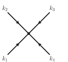
Figure 1: Scalar 4-field vertex

$$\tilde{\Gamma}(k_{1},k_{2},k_{3},k_{4};a) = i(2\pi)^{n}\frac{\lambda}{2}\,a_{\nu}\Bigg{[}\frac{a_{\nu}}{a^{2}}+\frac{1}{4}\bigg{(}k_{4\mu}k_{3\nu}+k_{3\mu}k_{4\nu}-2\delta_{\mu\nu}k_{4\rho}k_{3\rho}$$ (4.48)

$$+\frac{1}{2}(k_{2\mu}k_{4\nu}-k_{4\mu}k_{2\nu}+k_{2\mu}k_{3\nu}-k_{3\mu}k_{2\nu})\bigg{)}\partial_{\mu}^{k_{1}}$$

$$+\frac{1}{4}\bigg{(}k_{4\mu}k_{3\nu}+k_{3\mu}k_{4\nu}-2\delta_{\mu\nu}k_{4\rho}k_{3\rho}$$

$$+\frac{1}{2}(k_{1\mu}k_{4\nu}-k_{4\mu}k_{1\nu}+k_{1\mu}k_{3\nu}-k_{3\mu}k_{1\nu})\bigg{)}\partial_{\mu}^{k_{2}}$$

$$+\frac{1}{4}\bigg{(}k_{1\mu}k_{2\nu}+k_{2\mu}k_{1\nu}-2\delta_{\mu\nu}k_{1\rho}k_{2\rho}\bigg{)}(\partial_{\mu}^{k_{3}}+\partial_{\mu}^{k_{4}})\Bigg{]}\delta^{(n)}(k_{1}+k_{2}-k_{3}-k_{4}),$$

where we denote $\partial_{\mu}^{k}=\frac{\partial}{\partial k_{\mu}}$, and all four momenta $k_{i}$ are flowing into the vertex. Both couplings, $\xi$ and $\lambda$ have to be dimensionally regularized.

4.1.2 Feynman rules (B): $\kappa$-deformed momentum addition law

Next, we discuss the notion which anticipates the induced momentum conservation law on $\kappa$-space, within our hybrid approach. Namely, the $\delta$-function in (4.48) comes from the contraction of fields, where the momentum conservation should be obeyed in accordance with the $\kappa$-deformed momentum addition rule [18, 19, 43]. We have two cases for summation/subtraction of 4-vectors $k^{\mu}$ with respect to the physical situation of four particles and/or quantum fields propagating in space with respect to an interaction point:
(I) all particle momenta flowing into the vertex, as given in Fig. 1

$$k_{1\mu}+k_{2\mu}+k_{3\mu}+k_{4\mu}=0\;\;\to\;\;k_{1\mu}\oplus k_{2\mu}\oplus k_{3\mu}\oplus k_{4\mu}=0\,,$$ (4.49)

(II) the process of scattering ”2 particle $\to$ 2 particle”, where we have

$$(k_{1\mu}+k_{2\mu})-(k_{3\mu}+k_{4\mu})=0\,\;\;\to\;\;(k_{1\mu}\oplus k_{2\mu})\ominus(k_{3\mu}\oplus k_{4\mu})=0\,.$$ (4.50)

Having obtained the Feynman rules (4.46) and (4.48), we have completed the first stage of our program, that is to deduce the free propagation and interaction properties of the model by using the standard quantization.

At this point we turn to the second part, which includes the effective description of the statistics of particles described by the model. As already indicated before, the statistics of particles is twisted in $\kappa$-space [24, 25, 37, 42], with the deformation being encoded within the nonabelian momentum addition rule. It is known that the rule for addition of momenta is governed by the coproduct structure of the Hopf algebra in question. In our case, the relevant Hopf algebra is the $\kappa$-Poincaré algebra and the corresponding coalgebra structure is given by (2.18), (2.19), and (2.22), (2.23), respectively. In particular, the coproduct (2.18) for translation generators determines the required momentum addition rule, which in momentum space and up to the first order in deformation $a$, from (2.22) and (2.25), yields:

$$S(p_{\mu}) = -iS(\partial_{\mu})=-p_{\mu}-a_{\mu}p^{2}+(ap)p_{\mu}+{\mathcal{O}}(a^{2})\,,$$ (4.51)

$$(p_{\mu}\oplus k_{\mu}) = (p+k)_{\mu}+(ak)p_{\mu}-a_{\mu}(pk)+{\mathcal{O}}(a^{2})\,.$$ (4.52)

The second equation (4.52) states the nonabelian momentum addition rule, while $S(p)$ is the antipode with the property $p^{\mu}\oplus S(p^{\mu})=0$. Since commutativity in momentum space is not satisfied, i.e. $k\oplus p\not=p\oplus k$, a certain ordering has to be implemented. However, instead of implementing a possibly complicated unknown ordering, we shall proceed in the most simple way by taking into account all possible type of contributions; for example $k\oplus p\oplus q$, $p\oplus k\oplus q$, etc. Combining (4.51) and (4.52), we obtain the following momentum subtraction rule:

$$p_{\mu}\ominus k_{\mu} \equiv (p\oplus S(k))_{\mu}=(p-k)_{\mu}(1-ak)+a_{\mu}(pk-k^{2})+{\mathcal{O}}(a^{2})\,.$$ (4.53)

This enables us to rewrite the energy-momentum conservation which is supposed to be satisfied at each vertex. Thus, if two external momenta $k_{1}$ and $k_{2}$ flow into the vertex and the other two external momenta $k_{3}$ and $k_{4}$ flow out of the vertex, then, writing in components, we have the induced momentum conservation law (4.50), which corresponds to our physical situation .

In order to obtain the expressions for the $\delta$-functions in Feynman rules, we are starting with

$$\delta^{(n)}(p\ominus k)=\sum_{i}\Bigg{|}\det\Bigg{(}\frac{\partial{(p\ominus k)}_{\mu}}{\partial p_{\nu}}\Bigg{)}_{p=q_{i}}\Bigg{|}^{-1}\delta^{(n)}(p-q_{i})\,,$$ (4.54)

where we have to sum over all zeros $q_{i}$ for the expression in the argument of the $\delta$-function. Since there is only one zero at $q_{i}=k$, with the help of subtraction rule (4.53), we find the following first order contribution to the above $\delta^{(n)}$-function

$$\delta^{(n)}(p\ominus k)=\frac{\delta^{(n)}(p-k)}{{(1-ap)}^{n-1}}=(1+(n-1)ap+\mathcal{O}(a^{2}))\delta^{(n)}(p-k)\,.$$ (4.55)

It was shown in [54] that the star product $\star_{h}$ (3.35) breaks translation invariance (in the sense of [18]). However, this feature does not show up until computations are extended to second order in the deformation parameter $a$. The important point is that translation invariance is conserved within the first order deformation. Since we are carrying out our investigation in exactly this order, we are allowed to invoke the energy momentum conservation albeit in a modified form, dictated by the modified coproduct structure and by the oscillator term. Relations between Hopf algebra symmetries and conservation laws are an important subject of investigation. This is the issue of generalizing the Noether theorem, thus the whole subject is still appealing [85].

With the idea of implementing the new physical features that have just been described, we modify the Feynman rule (4.48). Taking into account all possible contributions, with the help of (4.52) and (4.53), and choosing the following replacement of $\delta$-function from (4.48) [17, 19, 20, 86],

$$\delta^{(n)}(k_{1}+k_{2}-k_{3}-k_{4})\rightarrow\delta^{(n)}((k_{1}\oplus k_{2})\ominus(k_{3}\oplus k_{4}))+\delta^{(n)}((k_{1}\oplus k_{2})\ominus(k_{4}\oplus k_{3}))\,,$$ (4.56)

we obtain the hybrid Feynman rule which obeys the $\kappa$-deformed momentum addition/subtraction rule via sum of $\delta$-functions (4.56):

$$\tilde{\Gamma}(k_{1},k_{2},k_{3},k_{4};a) = i(2\pi)^{n}\frac{\lambda}{2}\,a_{\nu}\Bigg{[}\frac{a_{\nu}}{a^{2}}+\frac{1}{4}\bigg{(}k_{4\mu}k_{3\nu}+k_{3\mu}k_{4\nu}-2\delta_{\mu\nu}k_{4\rho}k_{3\rho}$$ (4.57)

$$+\frac{1}{2}(k_{2\mu}k_{4\nu}-k_{4\mu}k_{2\nu}+k_{2\mu}k_{3\nu}-k_{3\mu}k_{2\nu})\bigg{)}\partial_{\mu}^{k_{1}}$$

$$+\frac{1}{4}\bigg{(}k_{4\mu}k_{3\nu}+k_{3\mu}k_{4\nu}-2\delta_{\mu\nu}k_{4\rho}k_{3\rho}$$

$$+\frac{1}{2}(k_{1\mu}k_{4\nu}-k_{4\mu}k_{1\nu}+k_{1\mu}k_{3\nu}-k_{3\mu}k_{1\nu})\bigg{)}\partial_{\mu}^{k_{2}}$$

$$+\frac{1}{4}\bigg{(}k_{1\mu}k_{2\nu}+k_{2\mu}k_{1\nu}-2\delta_{\mu\nu}k_{1\rho}k_{2\rho}\bigg{)}(\partial_{\mu}^{k_{3}}+\partial_{\mu}^{k_{4}})\Bigg{]}$$

$$\times\bigg{[}\delta^{(n)}((k_{1}\oplus k_{2})\ominus(k_{3}\oplus k_{4}))+\delta^{(n)}((k_{1}\oplus k_{2})\ominus(k_{4}\oplus k_{3}))\bigg{]}\,.$$

In the above, the sum of $\delta$-functions represents all mutually different physical situations.

The $\delta$-functions in (4.57), should in principle come from the contraction of fields quite naturally, if the noncommutative version of the LSZ formalism is applied to our model. Since such a formalism has not been developed so far, we choose to follow an approach that kind of combines the standard quantum field theory consideration (used when treating terms in the Lagrangian linear in $a$ as small perturbations) with the peculiarities resulting from the $\kappa$-deformed statistics of particles. The latter part is realized through embedding a nonabelian momentum-energy conservation within the 4-point vertex function. That approach may seem as a hybrid construction arising from trying to move our understanding one step forward towards a complete quantum theory on noncommutative spaces in general. In this sense, such an approach can serve as an intermediate step bridging the gap between the standard quantum field theory and a complete field theory on $\kappa$-space in a similar way as for example the semiclassical theory of radiation can be considered as a cross-over towards the quantum theory of radiation. In following the described path we have to rely in part on intuition, especially when peculiarities of $\kappa$-space statistics have to be taken into account.

The Feynman rule (4.57) now appears to be consistent with the energy-momentum conservation that respects the $\kappa$-deformed momentum addition rule. In order to obtain the complete expression for the $\delta$-functions appearing in (4.57), we are proceeding in two steps. First, with the help of (4.52) and (4.55), up to linear order in $a$, and with $j,l=3,4;\,j\not=l$, we have:

$$\delta^{(n)}((k_{1}\oplus k_{2})\ominus(k_{j}\oplus k_{l})) = \frac{\delta^{n}((k_{1}\oplus k_{2})-(k_{j}\oplus k_{l}))}{{\bigg{(}1-a(k_{1}\oplus k_{2})\bigg{)}}^{n-1}}$$

$$=\frac{\delta^{(n)}((k_{1}\oplus k_{2})-(k_{j}\oplus k_{l}))}{{\bigg{[}1-\bigg{(}a(k_{1}+k_{2})+(ak_{1})(ak_{2})-a^{2}(k_{1}k_{2})+{\mathcal{O}}(a^{3})\bigg{)}\bigg{]}}^{n-1}}$$

$$=(1+(n-1)a(k_{1}+k_{2})+{\mathcal{O}}(a^{2}))\delta^{(n)}((k_{1}\oplus k_{2})-(k_{j}\oplus k_{l}))\,.$$

The second step is to compute the $\delta$-functions from (4.1.2) in the same way as we computed the one in (4.55):

$$\delta^{(n)}((k_{1}\oplus k_{2})-(k_{j}\oplus k_{l}))=\sum_{i}\Bigg{|}\det\Bigg{(}\frac{\partial{((k_{1}\oplus k_{2})-(k_{j}\oplus k_{l})}_{\mu}}{\partial k_{1\nu}}\Bigg{)}_{k_{1}=q_{i}}\Bigg{|}^{-1}\delta^{(n)}(k_{1}-q_{i})\,,$$ (4.59)

where we have to sum up over all zeros $q_{i}$ for the expression in the argument of $\delta$-function.

To proceed, we shall choose specific values for the momenta $k_{2}=k_{3}=\ell$, which we need for the evaluation of the tadpole diagram. Since there are no zeros for the delta function $\delta^{(n)}((k_{1}\oplus\ell)-(\ell\oplus k_{4}))$, the only contribution comes from the second combination $\delta^{(n)}((k_{1}\oplus\ell)-(k_{4}\oplus\ell))$. In order to perform that computation, we start with (4.52) and orient the vector $a$ in the direction of time, $a=(0,...,0,ia_{0}).$ Then due to covariance, the obtained result will also be valid for an arbitrary orientation of $a$. Hence

$$\det{\left(\frac{\partial{((k_{1}\oplus\ell)-(k_{4}\oplus\ell))}_{\mu}}{\partial k_{1\nu}}\right)}_{k_{1}=k_{4}} = \left|\begin{array}[]{ccccc}1&~{}-ia_{0}\ell_{1}&\cdot\cdot\cdot&~{}-ia_{0}\ell_{n-2}&~{}-ia_{0}\ell_{n-1}\\ 0&1+a\ell&\cdot\cdot\cdot&0&0\\ \cdot&\cdot&\cdot\cdot\cdot&\cdot&\cdot\\ \cdot&\cdot&\cdot\cdot\cdot&\cdot&\cdot\\ 0&0&\cdot\cdot\cdot&1+a\ell&0\\ 0&0&\cdot\cdot\cdot&0&1+a\ell\\ \end{array}\right|$$ (4.66)

$$= {(1+a\ell)}^{n-1}.$$ (4.67)

Since there is only one zero, at $q_{i}=k_{4}$, we find

$$\delta^{(n)}((k_{1}\oplus\ell)-(k_{4}\oplus\ell))=\frac{\delta^{(n)}(k_{1}-k_{4})}{{(1+a\ell)}^{n-1}}=\bigg{(}1-(n-1)a\ell\bigg{)}\delta^{(n)}(k_{1}-k_{4})+\mathcal{O}(a^{2})\,,$$ (4.68)

which gives us the final expression for the $\delta$-function in (4.57) via (4.1.2), up to first order in $a$:

$$\delta^{(n)}((k_{1}\oplus\ell)\ominus(k_{4}\oplus\ell)) = \bigg{(}1+(n-1)a(k_{1}+\ell)\bigg{)}\frac{\delta^{(n)}(k_{1}-k_{4})}{{(1+a\ell)}^{n-1}}+\mathcal{O}(a^{2})$$ (4.69)

$$= (1+(n-1)ak_{1})\delta^{(n)}(k_{1}-k_{4})+\mathcal{O}(a^{2})\,.$$

In the above expression the dependences on $\ell$ drop out as we expected, thus showing the consistency of the hybrid Feynman rule derivation. The remaining factor $(1+(n-1)ak_{1})$ in (4.69) is due to the $\kappa$-space twisted particle statistics of our hybrid approach.

4.2 Massive scalar field propagation

4.2.1 Tadpole diagram: standard momentum conservation

In order to compute the tadpole diagram from Fig. 2, using dimensional regularization technique, we have to introduce in the action (3.38) $new$ dimensionfull regularization masses, denoted by $\mu$ for the coupling $\lambda$, and by $\mu^{\prime}$ for $\xi^{2}$, respectively. In accordance with quantum field theory [87], the regularization of the $\phi^{4}$ model requires that they are given in the following form:

$$\lambda_{new} = \lambda_{old}(\mu^{2})^{\frac{n}{2}-2}\;\;\;\to\;\;\;(\mu^{2})^{2-\frac{n}{2}}\lambda\,,\;\;\;\lambda=\lambda_{new}\,,$$ (4.70)

$$\xi_{new} = \xi_{old}({\mu^{\prime}}^{2})^{\frac{n}{2}-4}\;\;\;\to\;\;\;({\mu^{\prime}}^{2})^{4-\frac{n}{2}}\xi\,,\;\;\;\xi=\xi_{new}\,.$$ (4.71)

Here $\mu^{\prime}$ is defined in such a way that the new parameters are dimensionless.

In this paper, we shall further restrict our computation only to the first order contribution of the two-point function ${\Pi}^{a,\xi}_{2}$ in our $\lambda\phi^{4}$ model, (3.38), corresponding to the tadpole diagram depicted in Fig. 2:

$$\Pi^{a,\xi}_{2}={\Pi}^{0,0}_{2}+{\Pi}^{a\neq 0,0}_{2}+{\Pi}^{0,\xi\neq 0}_{2}+{\Pi}^{a\neq 0,\xi\neq 0}_{2}=\int\frac{d^{n}k_{2}}{(2\pi)^{n}}\frac{d^{n}k_{3}}{(2\pi)^{n}}\,\tilde{\Gamma}(k_{1},k_{2},k_{3},k_{4};a,\mu)G^{\xi}(k_{2},k_{3};\mu^{\prime})\,.$$ (4.72)

In general, the one-loop integral (4.72) produces four different contributions, where for $G^{\xi}(k_{2},k_{3};\mu^{\prime})$ we are using the expanded expression (4.46) further on. In computing the first two terms from (4.72), we assume momentum conservation, $k_{1}+k_{2}=k_{3}+k_{4}$ and $k_{2}=k_{3}=\ell$. Thus we have

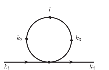
Figure 2: Scalar 4-field tadpole

$${\Pi}^{a,0}_{2}=\int\frac{d^{n}\ell}{(2\pi)^{n}}\;\tilde{\Gamma}(k_{1},\ell,\ell,k_{4};a,\mu)\,\frac{i}{\ell^{2}+m^{2}}\,.$$ (4.73)

First, we need $\tilde{\Gamma}$ from the Feynman rule (4.48), in accordance with the notations from Fig. 1; that is for incoming momenta $k_{1}$ and outgoing momenta $k_{4}$ we have to replace $k_{3}\to-k_{3}=-\ell$ and $k_{4}\to-k_{4}$. Thus, we have

$$\tilde{\Gamma}(k_{1},\ell,\ell,k^{out}_{4};a,\mu)=i(2\pi)^{n}\mu^{4-n}\;\frac{\lambda}{2}\,\Bigg{\{}1+a_{\nu}\frac{1}{8}\bigg{[}\bigg{(}k_{4\mu}k_{1\nu}-k_{1\mu}k_{4\nu}\bigg{)}\partial^{\ell}_{\mu}$$

$$- 2\bigg{(}{\ell}_{\mu}k_{4\nu}-3\ell_{\nu}k_{4\mu}+8\delta_{\mu\nu}k_{4\rho}\ell_{\rho}\bigg{)}\partial^{k_{1}}_{\mu}-2\bigg{(}\ell_{\mu}k_{1\nu}+k_{1\mu}\ell_{\nu}-2\delta_{\mu\nu}k_{1\rho}\ell_{\rho}\bigg{)}\partial_{\mu}^{k_{4}}$$

$$+ \bigg{(}\ell_{\mu}(2k_{4}-k_{1})_{\nu}+\ell_{\nu}(2k_{4}-3k_{1})_{\mu}-4\delta_{\mu\nu}(k_{4}-k_{1})^{\rho}\ell_{\rho}\bigg{)}\partial^{\ell}_{\mu}\bigg{]}\Bigg{\}}\delta^{(n)}(k_{1}-k_{4})\,.$$

In order to obtain $\tilde{\Gamma}(k_{1},\ell,\ell,k^{in}_{4};a,\mu)$ we just have to replace $k_{4}\to-k_{4}$ in (4.2.1).

As a next step, we compute $\Pi^{a,\xi}_{2}$ straightforwardly. Employing integration by parts in (4.73) and using the dimensional regularization scheme, we obtain

$$\Pi^{0,0}_{2} = -\frac{\lambda}{2}\,I_{0}\,,$$ (4.75)

$$\Pi^{a\neq 0,0}_{2} = -\frac{\lambda}{2}\Bigg{\{}\frac{3}{8}{(aK)}I_{0}-\frac{1}{4}{(aK)}\bigg{(}{\delta}_{\mu\nu}-\frac{a_{\mu}K_{\nu}}{(aK)}\bigg{)}I_{2,\mu\nu}\Bigg{\}}\,,$$ (4.76)

where $K=2k_{4}-k_{1}$. The oscillator contribution from the $\xi$-term has been obtained by a rude approximation of (4.72). That is, from

$${\Pi}^{0,\xi\neq 0}_{2}=-i\int\frac{d^{n}\ell}{(2\pi)^{n}}\;\tilde{\Gamma}(k_{1},\ell,\ell,k_{4};a,\mu)\,\frac{\xi^{2}}{(\ell^{2}+m^{2})^{2}}\partial_{\ell}^{2}\delta^{(n)}(\ell)\,,$$ (4.77)

after integrating by parts, we have found

$$\Pi^{0,\xi\neq 0}_{2} = -\frac{\lambda}{2}\xi^{2}\frac{(8n)({\mu^{\prime}}^{2})^{4-\frac{n}{2}}}{m^{6}}\,.$$ (4.78)

In the above equations, we have omitted the factor $(2\pi)^{n}\delta^{(n)}(k_{1}-k_{4})$ for simplicity. For $n=4-\epsilon$, we have the well known integrals

$$I_{0} = (\mu^{2})^{2-\frac{n}{2}}\int\frac{d^{{n}}\ell}{(2\pi)^{n}}\frac{1}{\ell^{2}+m^{2}}=\frac{m^{2}}{(4\pi)^{2}}\Bigg{[}\Bigg{(}\frac{4{\pi}{\mu}^{2}}{m^{2}}\Bigg{)}^{\frac{\epsilon}{2}}\Gamma(-1+\frac{\epsilon}{2})\;{{\Bigg{]}}_{\epsilon\to 0}}$$ (4.79)

$$= \frac{-1}{8\pi^{2}}m^{2}\Bigg{[}\frac{1}{\epsilon}+\frac{\psi(2)}{2}+{\rm log}\sqrt{\frac{4\pi\mu^{2}}{m^{2}}}+...\Bigg{]}\,,$$

$$I_{2,\mu\nu} = (\mu^{2})^{2-\frac{n}{2}}\int\frac{d^{n}\ell}{(2\pi)^{n}}\frac{\ell_{\mu}\ell_{\nu}}{(\ell^{2}+m^{2})^{2}}=\frac{1}{2}\delta_{\mu\nu}I_{0}\,,\;\;\;\delta_{\mu\nu}\delta_{\mu\nu}=n\,,$$ (4.80)

with a simple pole at $\epsilon=0$. Thus the expression (4.79) is divergent in the UV cut-off.

The non-vanishing contributions come from the commutative cases, that is from (4.75), and from harmonic oscillator term (4.78) which is finite for finite scalar field mass. The integrals (4.79) and (4.80) for $n=4$ give $\Pi^{a\neq 0,0}_{2}=0$, producing in the case $\xi=0$, very well known commutative $\lambda\phi^{4}$ theory result (4.75). All contributions proportional to $a$, coming from $\kappa$-Minkowski NC $\phi^{4}$ theory cancel out, as one would naively expect by inspecting the vertex weight (4.2.1).

Clearly, the one loop computation has to be modified by anticipating the momentum conservation on $\kappa$-space. To illustrate that something nonstandard appears in our model (4.48), we start with the general one-loop integral (4.72). It should be noted that one cannot integrate over $k_{3}$ using the first delta $\delta^{(n)}(k_{2}-k_{3})$ – from the propagator – and replace $k_{3}$ by $k_{2}$ in the above expression as it stands, because of the derivative with respect to $k_{2}$. So, in a first step of the computation we are using a simple trick

$$\partial_{\mu}^{k_{1}}\delta^{(n)}(k_{1}+k_{2}-k_{3}-k_{4}) = \partial_{\mu}^{k_{2}}\delta^{(n)}(k_{1}+k_{2}-k_{3}-k_{4})\,,$$

$$\partial_{\mu}^{k_{1}}\delta^{(n)}(k_{1}+k_{2}-k_{3}-k_{4}) = -\partial_{\mu}^{k_{3}}\delta^{(n)}(k_{1}+k_{2}-k_{3}-k_{4})\,,\;{\rm etc.,}$$ (4.81)

and than we rewrite (4.48) and (4.46) as follows:

$$\tilde{\Gamma}(k_{1},k_{2},k_{3},k_{4};a)G^{\xi}(k_{2},k_{3})=$$

$$\Bigg{\{}i(2\pi)^{n}\frac{\lambda}{4}\Bigg{[}1+a_{\nu}\bigg{(}2(-k_{1\mu}k_{2\nu}-k_{2\mu}k_{1\nu}+k_{3\mu}k_{4\nu}+k_{4\mu}k_{3\nu}+2\delta_{\mu\nu}(k_{1\rho}k_{2\rho}-k_{3\rho}k_{4\rho}))$$

$$+\frac{1}{2}(k_{1\mu}k_{3\nu}-k_{3\mu}k_{1\nu}+k_{2\mu}k_{3\nu}-k_{3\mu}k_{2\nu}+k_{1\mu}k_{4\nu}-k_{4\mu}k_{1\nu}+k_{2\mu}k_{4\nu}-k_{4\mu}k_{2\nu})\bigg{)}\partial_{\mu}^{k_{1}}\Bigg{]}$$

$$\times\delta^{(n)}(k_{1}+k_{2}-k_{3}-k_{4})\Bigg{\}}\bigg{[}\frac{i}{k_{2}^{2}+m^{2}}\bigg{(}1-\frac{\xi^{2}}{(k_{2}^{2}+m^{2})}\partial^{2}_{k_{3}}\bigg{)}\delta^{(n)}(k_{2}-k_{3})\bigg{]}\,.$$ (4.82)

For the part independent of $\xi$, we obtain after performing the integration over $k_{3}$ in (4.82) the following expression:

$$\Pi^{a\neq 0,0}_{2}=-\frac{\lambda}{8(2\pi)^{n}}((ak_{1})k_{4}-(ak_{4})k_{1})_{\mu}\bigg{[}\partial_{\mu}^{k_{1}}\delta^{(n)}(k_{1}-k_{4})\bigg{]}\int\frac{d^{n}k_{2}}{k_{2}^{2}+m^{2}}\,,$$ (4.83)

where $k_{1}$ and $k_{4}$ are external momenta. This expression is quadratically divergent in the UV cut-off representing a quantum loop modification of the free action (3.38), which can be nonzero because of the momentum conservation violation at the vertex. The next term of (4.82), is obtained after partial integration:

$${\Pi}^{0,\xi\neq 0}_{2}=-\frac{\lambda\xi^{2}}{4(2\pi)^{n}}\bigg{[}\partial^{2}_{k_{1}}\delta^{(n)}(k_{1}-k_{4})\bigg{]}\int\;\frac{d^{n}k_{2}}{(k_{2}^{2}+m^{2})^{2}}\,.$$ (4.84)

It is logarithmically divergent in $n=4$ dimensions. The last term depends on both deformation parameters, $a$ and $\xi$, it reads

$${\Pi}^{a\neq 0,\xi\neq 0}_{2} = -\frac{\lambda\xi^{2}}{8(2\pi)^{n}}a_{\nu}\bigg{[}\bigg{(}\partial^{2}_{k_{1}}\partial_{\mu}^{k_{1}}\delta^{(n)}(k_{1}-k_{4})\bigg{)}(k_{1\mu}k_{4\nu}-k_{4\nu}k_{1\mu})$$ (4.85)

$$-4\bigg{(}\partial^{k_{1}}_{\sigma}\partial_{\mu}^{k_{1}}\delta^{(n)}(k_{1}-k_{4})\bigg{)}\bigg{(}2(\delta_{\mu\sigma}k_{4\nu}+\delta_{\nu\sigma}k_{4\mu}-2\delta_{\mu\nu}k_{4\sigma})$$

$$\hskip 28.45274pt+\frac{1}{2}(\delta_{\nu\sigma}k_{1\mu}-\delta_{\mu\sigma}k_{1\nu})\bigg{)}\bigg{]}\int\frac{d^{n}k_{2}}{(k_{2}^{2}+m^{2})^{2}}\,,$$

which is also logarithmically divergent in $n=4$ dimensions. The one-loop corrections (4.84)-(4.85) have to be included in the action as counterterms. Their structure is different from the tree-level terms, and therefore the tree-level action is not stable under 1-loop quantum corrections. For this reason, we have to question the approximations we have employed: namely the expansion of the action up to first order in the deformation parameter $a$ and the expansion of the propagator up to first order in $\xi$. The results (4.75) and (4.76) (as well as the result (4.86) that will follow shortly) are obtained directly from (4.73). We assume that (4.73) replaces the expression (4.72) for $\xi=0$. As for (4.78) (and (4.87)), it is a rude estimate of what the $\xi$ term would produce. It is obtained by making approximations in (4.72), by approximating/adjusting the form of the propagator (4.46) and by using the $\kappa$-deformed addition/subtraction of momenta instead of the commutative one. The difference between (4.78) and (4.87) is that unlike the former expression, the latter one is obtained by making use of the $\kappa$-deformed addition/subtraction rule for momenta. Due to the results (4.83)-(4.85) we obviously stumbled across the momentum nonconservation. Such results seem to favor our hybrid approach.

4.2.2 Tadpole diagram: $\kappa$-deformed momentum conservation

In the following computation of the tadpole diagram from Fig. 2, we fully implement the hybrid approach. That is the notion that standard momentum conservation is not satisfied, i.e. we use induced momentum conservation on $\kappa$-space represented within the $\delta$-functions in (4.56). However, in accordance with our hybrid approach, at the end undeformed momentum conservation has to be applied. The general one-loop integral (4.72) can be roughly reduced to two terms, namely (4.73) and (4.77).

In the next step, we are applying integration by parts, which is possible due to the notion that the remaining integral in (4.72) is an effective action of the given one-loop quantum process. This of course plays an essential role in our hybrid approach. Performing the computation of all terms in the tadpole one-loop integral (4.73) with Feynman rule (4.57) and $\delta$-function (4.69) and for an arbitrary number of dimensions $n$, we obtain the following first order result:

$$\Pi^{0,0}_{2}+\Pi^{a\neq 0,0}_{2} = -\frac{\lambda}{2}\bigg{[}(1+(n-1)ak_{1})+\frac{1}{2}(1-\frac{n}{4})(ak_{1}-2ak_{4})\bigg{]}\,I_{0}$$ (4.86)

$$\Pi^{0,\xi\neq 0}_{2}+\Pi^{a\neq 0,\xi\neq 0}_{2} = -\frac{\lambda}{2}\xi^{2}\frac{8n({\mu^{\prime}}^{2})^{4-\frac{n}{2}}}{m^{6}}(1+(n-1)ak_{1})\,.$$ (4.87)

The first terms in (4.86) and (4.87) for $n=4$ correspond to the results (4.75) and (4.78) from the previous subsection. From the above formulas it is clear that there exist non-vanishing contributions even for $n=4$ dimensions. They are arising via the $\kappa$-deformed momentum conservation rule, entering through the deformed $\delta$-function (4.69) in the hybrid Feynman rule (4.57), and from the harmonic oscillator term in the action (3.38) via the modified propagator (4.46).

For $n=4-\epsilon$, we obtain a modified expression for the tadpole in Fig. 2 in the limit $\epsilon\to 0$, where the $1/\epsilon$-divergence is explicitly isolated. For conserved external momentum in accordance with (4.69), i.e. for $k_{1}=k_{4}\equiv k$, from (4.79), (4.86) and (4.87) we finally have,

$${\Pi}^{a,\xi}_{2}=\frac{\lambda m^{2}}{32\pi^{2}}(1+3ak)\Bigg{[}\frac{2}{\epsilon}+\psi(2)+{\rm log}\frac{4\pi\mu^{2}}{m^{2}}-\frac{9}{4}\frac{ak}{1+3ak}-(4-\epsilon)128\pi^{2}\frac{\xi^{2}{\mu}^{4-\epsilon}}{m^{8}}\Bigg{]}\,,$$ (4.88)

where for simplicity we have used $\mu^{\prime}=\mu$, and in the $\xi$-term we retain the explicit $\epsilon$-dependence in order to keep dimensional and/or limiting procedure under control. The parts above represent modifications of the scalar field self-energy and explicitly depend on the regularization parameter, the mass of the scalar field, the magnitude of the translation invariance breaking, and it contains a correction $ak$ due to the dependence on the energy $|k|$, where actual scalar field self-energy modification occurs. The dependence of (4.88) on the $\kappa$-deformation parameter $a$ enters explicitly, as we expected. Note that there is no need to do renormalization at the point $(1+3ak)\to 0$.

The result (4.88) is next discussed in the framework of Green’s functions. Generally we know that by summing all the 1PI contributions, for the modifications of the full free propagator (4.45), we get the following expression for the two-point connected Green’s function [87]

$$G_{(c,2)}^{a,\xi}(k_{1},k_{4}) = \bigg{[}\frac{i}{k_{1}^{2}+m_{1}^{2}}+\frac{i}{k_{1}^{2}+m_{1}^{2}}{\Pi}^{a,\xi}_{2}\frac{i}{k_{1}^{2}+m_{1}^{2}}+...\bigg{]}\,,$$ (4.89)

where, symbolically, $m_{1}^{2}=m^{2}+\xi^{2}\partial^{2}_{k_{1}}\delta^{(n)}(k_{1}-k_{4})$ represents the redefined mass. As an illustration we resume the above series in the limit $\xi\to 0$:

$$G_{(c,2)}^{a,\xi}(k_{1},k_{4}) {}_{\longrightarrow}^{\xi\to 0} \,(2\pi)^{n}\delta^{(n)}(k_{1}-k_{4})\bigg{[}\frac{i}{k_{1}^{2}+m^{2}-{\Pi}^{a,0}_{2}}\bigg{]}\,.$$ (4.90)

The genuine $1/\epsilon$ divergence in ${\Pi}^{a,\xi}_{2}$, can only be removed by introducing the following counter term $\delta m^{2}$:

$$\delta m^{2}\tilde{\phi}^{*}(k)\tilde{\phi}(k)=\frac{\lambda m^{2}}{32\pi^{2}}\Bigg{[}2(1+3ak)\frac{1}{\epsilon}+f\bigg{(}\frac{4-\epsilon}{2},\frac{\mu^{2}}{m^{2}},ak,\frac{\xi^{2}}{m^{4}}\bigg{)}\Bigg{]}\tilde{\phi}^{*}(k)\tilde{\phi}(k)\,,$$ (4.91)

where $f$ denotes an arbitrary dimensionless function, which is fixed by the renormalization conditions. Adding the contribution of the above counterterm to the previous expression (4.89) results during the renormalization procedure in the shift $m^{2}\to m^{2}+\delta m^{2}$ in (4.89)/(4.90), thus leading to

$${\tilde{G}}_{(c,2)}^{a,\xi}(k_{1},k_{4}) = \Bigg{[}G_{(c,2)}^{a,\xi}(k_{1},k_{4})+G_{(c,2)}^{a,\xi}(k_{1},k_{4})(-\delta m^{2})G_{(c,2)}^{a,\xi}(k_{1},k_{4})+...\Bigg{]}$$ (4.92)

$${}_{\longrightarrow}^{\xi\to 0} (2\pi)^{n}\delta^{(n)}(k_{1}-k_{4})\bigg{[}\frac{i}{k_{1}^{2}+m^{2}+\delta m^{2}-{\Pi}^{a,0}_{2}}\bigg{]}\,,$$

where ${\tilde{G}}_{(c,2)}^{a,\xi}$ denotes the Green’s function with the contribution from the counterterm incorporated.

However, since ${\Pi}^{a,\xi}_{2}$ was computed for the expanded free propagator (4.46), it is consistent to compute the two-point connected Green’s function under the same approximation. After the resummation of (4.89) and using (4.46), we obtain

$$G_{(c,2)}^{a,\xi}(k_{1},k_{4})=\frac{G^{\xi}}{1-G^{\xi}\;{\Pi}^{a,\xi}_{2}}\,.$$ (4.93)

In order to identify the proper counterterm for the above expression, we resume the series in (4.92), but with replacement (4.89) $\to$ (4.93), and the full free propagator $i/(k_{1}^{2}+m_{1}^{2})$ replaced with the expanded one (4.46), giving:

$${\tilde{G}}_{(c,2)}^{a,\xi}(k_{1},k_{4})=\frac{G^{\xi}}{1+G^{\xi}(\delta m^{2}-{\Pi}^{a,\xi}_{2})}\,.$$ (4.94)

In (4.94) $\delta m^{2}$ is a generic quantity. This is due to the fact that expression (4.88) also contains finite parts. The requirement $\delta m^{2}={\Pi}^{a,\xi}_{2}$ removes the infinity. Thus we have

$${\tilde{G}}_{(c,2)}^{a,\xi}(k_{1},k_{4})=\frac{G^{\xi}}{1+G^{\xi}\frac{\lambda m^{2}}{32\pi^{2}}\bigg{[}f-(1+3ak)\bigg{(}\psi(2)+{\rm log}\frac{4\pi\mu^{2}}{m^{2}}-\frac{9}{4}\frac{ak}{1+3ak}-512\pi^{2}\frac{\xi^{2}{\mu}^{4}}{m^{8}}\bigg{)}\bigg{]}}\,.$$

(4.95)

Precise extraction and removal of the genuine UV divergence is performed next via (4.91) in the context of the analysis of ${\tilde{G}}_{(c,2)}^{a,\xi}(k_{1},k_{4})$ for different energy regimes; that is from low energy to extremely high -Planck scale- energy propagation.

There is a very interesting property of expression (4.88) at extreme energies. Namely, there exists a term $(1+3ak)$ which for $(1+3ak\to 0)$ tends to zero linearly. For low energies and/or small $\kappa$-deformation $a$, i.e. for $ak=0$, (equivalent to $a=0$), which is far away from the point $(1+3ak=0)$, this is not the case.

Low energy limit
Using the finite combination $(\delta m^{2}-\Pi^{0,0}_{2})$ for low energy ($ak=0$), and at order $\lambda$

$$\delta m^{2}-{\Pi}^{0,0}_{2}=\frac{\lambda m^{2}}{32\pi^{2}}\Bigg{[}f-\psi(2)-{\rm log}\frac{4\pi\mu^{2}}{m^{2}}\Bigg{]}\,,$$ (4.96)

from (4.88) and (4.95), we get

$${\tilde{G}}_{(c,2)}^{0,\xi}(k_{1},k_{4})=\frac{G^{\xi}}{1+G^{\xi}\frac{\lambda m^{2}}{32\pi^{2}}\bigg{(}f-\psi(2)-{\rm log}\frac{4\pi\mu^{2}}{m^{2}}+512\pi^{2}\frac{\xi^{2}{\mu}^{4}}{m^{8}}\bigg{)}}\,,$$

(4.97)

while in the case $\xi=0$

$${\tilde{G}}_{(c,2)}^{0,0}(k_{1},k_{4})=\frac{(2\pi)^{4}\delta^{(4)}(k_{1}-k_{4})}{k_{1}^{2}+m^{2}\bigg{(}1+\frac{\lambda}{32\pi^{2}}\bigg{[}f-\psi(2)-{\rm log}\frac{4\pi\mu^{2}}{m^{2}}\bigg{]}\bigg{)}}\,.$$

(4.98)

This expression has a pole in Minkowski space, and we can define the renormalization condition by requiring that the inverse propagator at the physical mass is $k_{1}^{2}+m^{2}_{phys/low}$. This choice, in the case $\xi^{2}=0$, determines uniquely the sum of the residual terms in (4.96), which is in accordance with the result from commutative $\phi^{4}$ theory [87].

Planckian energy limit
At the limiting point $(1+3ak\to 0)$, which corresponds to extreme energy propagation $|k|$, where the components of the $\kappa$-deformation parameter $a_{\mu}$ are extremely small, of Planck length order, the divergence in (4.88) gets removed under the reasonable assumption that $(1+3ak)$ tends to zero with the same speed as $\epsilon$ does. That is, in the Planckian propagation energy limit

$$\frac{(1+3ak)\to 0}{\epsilon\to 0}\longrightarrow{\cal O}(1)\,,$$ (4.99)

the $1/\epsilon$ and $ak$ terms from (4.88) do contribute.

Assuming that our $\kappa$-noncommutativity is spatial, $a_{\mu}=(\vec{a},0)$, and using the momentum along the third axis $k_{\mu}=(0,0,E,iE)$, i.e. for $ak=Ea_{3}$, Eq. (4.88) in the Planckian propagation energy limit (4.99) gives

$$\Pi^{a,0}_{2}\,\bigg{|}_{(3Ea_{3}+1\to 0)}\longrightarrow\,\frac{\lambda m^{2}}{32\pi^{2}}\;\bigg{[}2-\frac{9}{4}ak\bigg{]}_{(3Ea_{3}+1\to 0)}\,,$$ (4.100)

producing the following modified Green’s function (4.90):

$$\Pi^{a,0}_{2}\,\bigg{|}_{(3Ea_{3}+1\to 0)}\to\frac{\lambda m^{2}}{32\pi^{2}}\,\frac{11}{4}\,\Rightarrow\;{\tilde{G}}_{(c,2)}^{a,0}(k_{1},k_{4})\bigg{|}_{(3Ea_{3}+1\to 0)}\simeq\frac{i(2\pi)^{4}\delta^{(4)}(k_{1}-k_{4})}{k_{1}^{2}+m^{2}\bigg{(}1-\frac{\lambda}{32\pi^{2}}\frac{11}{4}\bigg{)}}\,.$$ (4.101)

At exact zero-point $3Ea_{3}+1=0$ however, from (4.88) we obtain a different result

$$\Pi^{a,0}_{2}\,\bigg{|}_{(3Ea_{3}+1=0)}=\frac{\lambda m^{2}}{32\pi^{2}}\,\frac{3}{4}\,\;\;\Rightarrow\;\;{\tilde{G}}_{(c,2)}^{a,0}(k_{1},k_{4})\bigg{|}_{(3Ea_{3}+1=0)}\simeq\frac{i(2\pi)^{4}\delta^{(4)}(k_{1}-k_{4})}{k_{1}^{2}+m^{2}\bigg{(}1-\frac{\lambda}{32\pi^{2}}\frac{3}{4}\bigg{)}}\,.$$ (4.102)

For time-space noncommutativity with the time component of $\kappa$-deformation parameter $ia_{0}$ being also of order Planck length and vanishing space component, i.e. for $ak=-Ea_{0}$, Eq. (4.88) in the Planckian energy limit (4.99) yields the result:

$$\Pi^{a,0}_{2}\,|_{(3Ea_{0}-1\to 0)}\longrightarrow\,\frac{\lambda m^{2}}{32\pi^{2}}\;\bigg{[}2-\frac{9}{4}ak\bigg{]}_{(3Ea_{0}-1\to 0)}\,,$$ (4.103)

equivalent to (4.100), leading to final results which are identical to (4.101) and (4.102).

The existence of a linear type of limit $(1+3ak\to 0)$ which removes the genuine UV divergence $1/\epsilon$ is a new, previously unknown feature of NC $\kappa$-Minkowski $\phi^{4}$ theory at linear order in $a$. The mass shift is of a fixed value (4.100), independent of the function $f$, but dependent on the energy $|k|$ and the $\kappa$-deformation parameter $a$. Above expressions give $\kappa$-deformed dispersion relations, thus, (4.100)/(4.103) and (4.101)/(4.102) represent birefringence [65, 66] of the massive scalar field mode. Namely, neither of the finite terms in (4.95)-(4.98) do not contribute in the limit $(1+3ak)\to 0$, and the possibility of their internal cancellation is diminished. In this way, the birefringence of the massive scalar field mode arises as a genuine effect. The above inverse propagator determines the physical mass $m^{2}_{phys/Planck}$ at respected Planck scale energies.

5 Discussion and conclusion

Let us discuss the final outcome of the above constructed $\phi^{4}$ scalar field theory on the NC $\kappa$-deformed spacetime and describe the main results of this work.

First, we point out the most important new results:
(i) The integral measure problems on $\kappa$-Minkowski spacetime are avoided by the introduction of the new ${\star}_{h}$-product (3.35), which naturally absorbs the measure function due to the hermitian realization (3.32).
(ii) The trace-like property (the integral identity (3.36)) is valid for $\kappa$-deformed spaces, but only if one is dealing with the hermitian realization (3.32), as one should because only hermitian realizations have a physical meaning. Due to the integral identity (3.36), the only deformation with respect to the standard scalar field action comes from the interaction term in (3.37).
(iii) The action (3.38) includes a harmonic type of interaction term and is expanded up to first order in the deformation parameter $a$, producing an effective theory on commutative spacetime. Despite $\kappa$-deformation a mixture with the $\xi^{2}$ term in (3.37) via the ${\star}_{h}$ product, at first order in the $\kappa$-deformation parameter these two features of our model decouple completely in (3.38). The action (3.38) further produces modified equations of motion (3.40) and conserved deformed currents (3.41) due to the invariance under an internal symmetry. The above properties are very welcome.
(iv) The truncated $\kappa$-deformed action (3.38) does not possess the celebrated quantum effect of UV/IR mixing [45]. The lack of UV/IR mixing is a general feature of most of the NC gauge field theories expanded in terms of the deformation parameter. However, resummation of the expanded action could in principle restore the nonperturbative character of the model (see for example [60, 61, 62]), thus restoring the presence of UV/IR mixing in quantum loop computations. Under such circumstances UV/IR mixing would help in determining what the UV theory might be, that is, it would help to determine the UV completeness of the theory. It is important to note that UV/IR mixing connects NC gauge theories with Holography via UV and IR cutoffs, in a model independent way [57]. Both, UV/IR mixing and Holography, represent important windows to quantum gravity phenomena [57, 58, 59].
(v) Next, we discuss the result of the contribution of the tadpole diagram to the propagation and/or self-energy of our scalar field $\phi$ for arbitrary number of dimensions $n$, depicted in Fig. 2, as a function of $\kappa$-deformed momentum conservation law. This deformed conservation law originates from the deformed statistics on $\kappa$-Minkowski spacetime. Thus our approach represents kind of a hybrid approach of standard QFT and NCQFT, involving $\kappa$-deformed $\delta$-functions in the Feynman rules.
(vi) When we worked with the standard conservation of momenta (standard addition of momenta) and undeformed $\delta$-function, the contributions to the tadpole diagram to the first order in $a$ are zero. The deformed $\delta$-function can be written in terms of a leading term plus corrections in $a$. Since the Feynman rule (4.48) has already terms linear in $a$, we have to retain only the zeroth order term in the modified $\delta$-function, because otherwise we get terms of quadratic and higher orders in $a$ (and this is not what we are interested in). The only term where we need to take into account corrections linear in $a$ for the $\delta$-function is the leading order term in the Feynman rule (4.48). However, this term vanishes due to the integration over the loop momentum. Analyzing (4.83)-(4.85), we recognize that something nonstandard appears in the model for the tadpole integral at first order in $\lambda$ and $\kappa$-deformation $a$.
(vii) It appears that in the computation of the tadpole diagram integrals for $n=4$, all contributions linear in $a$ cancel each other automatically. For $n\not=4$ dimensions, the same contributions linear in $a$ become nonzero, regardless which momentum conservation rule is applied. However, the harmonic oscillator term from the action (3.38) modifies the mass term in the free propagator (4.45), thus producing an additional contribution (4.78) from the tadpole in Fig. 2. The propagation of the scalar field $\phi$ in $n=4$ dimensions also receives a modification from $\kappa$-deformation at linear order in the deformation parameter $a$, and it also receives a contribution due to the oscillator term.
(viii) In the final computation of the tadpole diagram depicted in Fig. 2, we fully implement the notion of our hybrid approach, that means that standard momentum conservation is not explicitly satisfied, and we have to use the momentum conservation on $\kappa$-spaces given by (4.50), while at the end of the computation the undeformed momentum conservation has to be applied. We have found non-vanishing contributions even for $n=4$ dimensions. They are arising from the harmonic oscillator term in the action (3.38) via the modified propagator (4.46), and the $\kappa$-deformed momentum conservation rule which enters through the deformed $\delta$-function in the hybrid Feynman rule (4.57). We have found the fully modified expression for the tadpole in Fig. 2 in the limit $\epsilon\to 0$, where the genuine $1/\epsilon$ (UV) divergence is explicitly isolated. For conserved external momenta, i.e. for $k_{1}=k_{4}\equiv k$, we obtain the two-point function (4.88), where the finite parts represent the modification of the scalar field self-energy $\Pi^{a,\xi}_{2}$ and depend explicitly on the regularization parameter $\mu^{2}$, the mass of the scalar field $m^{2}$, and the magnitude of the breaking of translational invariance $\xi^{2}$. The most important is that (4.88) contains the finite correction $ak$ due to the deformed statistics on $\kappa$-Minkowski spacetime, thus, via $ak$ term we obtain an explicit dependence on the scale of propagating energy involved $|k|=E$, and the $\kappa$-deformation parameter $a$, as we expected.
(ix) The two-point function (4.88) is next applied in the framework of two-point connected Green’s functions for three energy regimes, that is for low energies, for Planck scale energies, and for intermediate energies, respectively. For low energy scale and/or small $\kappa$-deformation $a$, i.e. for $ak\simeq 0$, which is far away from the point $(1+3ak=0)$, the dependence of the two-point Green’s function on the deformation parameter completely drops out (4.97). The genuine UV divergence in (4.88) has been removed by subtracting the counterterm $\delta m^{2}$ (4.91), from the previous contribution (4.89), or through shifting $m^{2}$ into $(m^{2}+\delta m^{2})$ in (4.90). In this case, the mass shift (4.97) could increase or decrease $m^{2}$ depending on the function $f$ and/or the parameter $\xi^{2}$.
(x) For energies within the limits $\frac{-1}{3a_{3}}\ll E\ll 0$ (or equivalently $\frac{1}{3a_{0}}\gg E\gg 0$), the full expression (4.88), with mass counterterm (4.91) has to be used in determining the Green’s function (4.92). In that particular case, the harmonic oscillator term in (4.88) will also give a non-negligible contribution. It’s coupling $\xi^{2}$ could be in principle determined by higher order contributions to the Green’s function. This is certainly an issue to be addressed in future work.
(xi) At Planckian energy scale, due to the existence of a linear type of limits $(1+3ak)\to 0$, we have new situation and, distinguish two cases. They are both new, previously unknown features of $\kappa$-deformed $\phi^{4}$ theory expanded up to linear order in the deformation parameter. In the first case we have the limit (4.99) which produces the self-energy and/or modified Green’s function (4.101).
(xii) Second case, where $1+3Ea_{3}=0$, represents in fact a genuine type of zero-point which exactly removes the UV divergence, yielding the self-energy and/or modified Green’s function (4.102). In both cases the mass term is shifted in the same direction, (the same sign!), but for a different amount, $+11/4$ versus $+3/4$, respectively. Or more precisely we can say that the mass shift during the limiting process $(3Ea_{3}+1\to 0)$ drops from the value proportional to $+11/4$ to $+3/4$.
(xiii) The results (4.101) and (4.102) are the same for two different choices of $\kappa$-noncommutativity, (with appropriate choice of referent system for momentum $k_{\mu}$), i.e. for $a_{\mu}=(0,0,a_{3},0)$ and $a_{\mu}=(0,0,0,ia_{0})$, respectively, since (4.100) and (4.103) are equivalent.
(xiv) At Planckian propagation energy scale $E\simeq\frac{-1}{3a_{3}}$, the contribution of the tadpole in Fig. 2 tends to a finite fixed value, between (4.101) and (4.102). Due to the effects of $\kappa$-Minkowski statistics, this depends on the direction of the propagation, the Planckian propagation energy and the deformation parameter $a$. In this way (4.100)/(4.103) and (4.101)/(4.102) represent $\kappa$-deformed dispersion relations and produce a birefringence effect [65, 66] of the massive scalar field mode, which arises as a genuine effect at first order in $a$. It is similar to the birefringence effect of the chiral fermion field in truncated Moyal $\star$-product theories [66].
(xv) Considering full renormalization, besides the $\delta m^{2}$ counterterm, the other divergent parts have to be added as counterterms to the action (3.38) as well:

$$\int d^{4}x\,({\cal L}+{\cal L}_{ct})=S[\phi_{B},m_{B},\lambda_{B},\xi_{B},a_{B}]\,,$$

where index $B$ denotes bare quantities and it is assumed that the counterterms can be absorbed by redefinition of the already existing parameters. That would include analysis of $4-point$ one-loop contributions, counterterms $(\mu^{2})^{2-\frac{n}{2}}\delta\lambda$ and $({\mu}^{2})^{4-\frac{n}{2}}\delta\xi$, as well as 2-loop expansion for the 2-point Green’s function with insertion of counterterms in multi-loop diagrams. However, the full renormalization of our action (3.38) is anyhow beyond the scope of this paper and it is planned for our next project.

Regarding the effects of statistics according to the described arguments, it is important to repeat that within first order in the deformation parameter $a$, effects of the deformed statistics on $\kappa$-Minkowski do appear in our hybrid model as semiclassical/hybrid behavior of the first order quantum effects, thus showing birefringence of the massive scalar field mode. We believe that this property of such a constructed model, is of importance for further possible research towards quantum gravity. At higher orders in $a$ the matter would become growingly interesting and complicated.

- [1] G. Amelino-Camelia, L. Smolin and A. Starodubtsev, Quantum symmetry, the cosmological constant and Planck scale phenomenology, Class. Quant. Grav. 21 (2004) 3095 [arXiv:hep-th/0306134].
- [2] L. Freidel, J. Kowalski-Glikman and L. Smolin, 2+1 gravity and doubly special relativity, Phys. Rev. D 69 (2004) 044001 [arXiv:hep-th/0307085.
- [3] L. Freidel and E. R. Livine, Ponzano-Regge model revisited. III: Feynman diagrams and effective field theory, Class. Quant. Grav. 23 (2006) 2021 [arXiv:hep-th/0502106].
- [4] L. Freidel and E. R. Livine, Effective 3d quantum gravity and non-commutative quantum field theory, Phys. Rev. Lett. 96 (2006) 221301 [arXiv:hep-th/0512113].
- [5] L. Freidel and S. Majid, Noncommutative Harmonic Analysis, Sampling Theory and the Duflo Map in 2+1 Quantum Gravity, Class. Quant. Grav. 25 (2008) 045006 [arXiv:hep-th/0601004].
- [6] J. Lukierski, H. Ruegg, A. Nowicki and V. N. Tolstoi, Q deformation of Poincare algebra, Phys. Lett. B 264 (1991) 331.
- [7] J. Lukierski, A. Nowicki and H. Ruegg, New quantum Poincare algebra and k deformed field theory, Phys. Lett. B 293 (1992) 344.
- [8] S. Majid and H. Ruegg, Bicrossproduct structure of Poincaré group and noncommutative geometry, Phys. Lett. B 334 (1994) 348 [arXiv:hep-th/9405107].
- [9] S. Zakrzewski, Quantum Poincaré group related to the -Poincaré algebra, J. Phys. A: Math. Gen 27 (1994) 2075.
- [10] J. Lukierski, H. Ruegg and W. J. Zakrzewski, Classical Quantum Mechanics Of Free Relativistic Systems, Annals Phys. 243 (1995) 90 [arXiv:hep-th/9312153].
- [11] G. Amelino-Camelia, Testable scenario for relativity with minimum-length, Phys. Lett. B 510 (2001) 255 [arXiv:hep-th/0012238].
- [12] G. Amelino-Camelia, Relativity in space-times with short-distance structure governed by an observer-independent (Planckian) length scale, Int. J. Mod. Phys. D 11 (2002) 35 [arXiv:gr-qc/0012051].
- [13] J. Magueijo and L. Smolin, Lorentz invariance with an invariant energy scale, Phys. Rev. Lett. 88 (2002) 190403 [arXiv:hep-th/0112090].
- [14] J. Magueijo and L. Smolin, Generalized Lorentz invariance with an invariant energy scale, Phys. Rev. D 67 (2003) 044017 [arXiv:gr-qc/0207085].
- [15] J. Kowalski-Glikman and S. Nowak, Doubly special relativity theories as different bases of -Poincaré algebra, Phys. Lett. B 539 (2002) 126 [arXiv:hep-th/0203040].
- [16] J. Kowalski-Glikman and S. Nowak, Non-commutative space-time of doubly special relativity theories, Int. J. Mod. Phys. D 12 (2003) 299 [arXiv:hep-th/0204245].
- [17] P. Kosinski, J. Lukierski and P. Maslanka, Local D = 4 field theory on -deformed Minkowski space, Phys. Rev. D 62 (2000) 025004 [arXiv:hep-th/9902037].
- [18] P. Kosinski, J. Lukierski and P. Maslanka, Local field theory on -Minkowski space, star products and noncommutative translations, Czech. J. Phys. 50 (2000) 1283 [arXiv:hep-th/0009120].
- [19] G. Amelino-Camelia and M. Arzano, Coproduct and star product in field theories on Lie-algebra non-commutative space-times, Phys. Rev. D 65 (2002) 084044 [arXiv:hep-th/0105120].
- [20] M. Daszkiewicz, K. Imilkowska, J. Kowalski-Glikman and S. Nowak, Scalar field theory on -Minkowski space-time and doubly special relativity, Int. J. Mod. Phys. A 20 (2005) 4925 [arXiv:hep-th/0410058].
- [21] M. Dimitrijevic, L. Jonke, L. Moller, E. Tsouchnika, J. Wess and M. Wohlgenannt, Deformed field theory on -spacetime, Eur. Phys. J. C 31 (2003) 129 [arXiv:hep-th/0307149].
- [22] S. Ghosh, A Lagrangian for DSR Particle and the Role of Noncommutativity, Phys. Rev. D74, 084019 (2006). [hep-th/0608206].
- [23] S. Ghosh, P. Pal, Deformed Special Relativity and Deformed Symmetries in a Canonical Framework, Phys. Rev. D75 (2007) 105021. [hep-th/0702159].
- [24] T. R. Govindarajan, K. S. Gupta, E. Harikumar, S. Meljanac and D. Meljanac, Deformed Oscillator Algebras and QFT in -Minkowski Spacetime, Phys. Rev. D 80 (2009) 025014, [arXiv:0903.2355 [hep-th]].
- [25] C. A. S. Young and R. Zegers, Covariant particle statistics and intertwiners of the -deformed Poincare algebra, Nucl. Phys. B 797 (2008) 537 [arXiv:0711.2206 [hep-th]].
- [26] M. Daszkiewicz, J. Lukierski, M. Woronowicz, “kappa-deformed statistics and classical fourmomentum addition law, Mod. Phys. Lett. A23 (2008) 653-665 [hep-th/0703200].
- [27] M. Arzano and A. Marciano, Fock space, quantum fields and -Poincaré symmetries, Phys. Rev. D 76 (2007) 125005 [arXiv:0707.1329 [hep-th]].
- [28] M. Daszkiewicz, J. Lukierski and M. Woronowicz, Towards quantum noncommutative -deformed field theory, Phys. Rev. D 77 (2008) 105007 [arXiv:0708.1561].
- [29] M. Daszkiewicz, J. Lukierski and M. Woronowicz, -deformed oscillators, the choice of star product and free -deformed quantum fields, J. Phys. A 42 (2009) 355201 [arXiv:0807.1992 [hep-th]].
- [30] M. Arzano and D. Benedetti, Rainbow statistics, Int. J. Mod. Phys. A 24 (2009) 4623 [arXiv:0809.0889 [hep-th]].
- [31] V. G. Drinfel’d, Hopf algebras and the quantum Yang-Baxter equation, Dokl. Akad. Nauk SSSR 283 (1985), no. 5, 1060-1064 (Russian); translation in Sov. Math. Dokl. 32 (1985) 254.
- [32] V. G. Drinfel’d, Quasi-Hopf algebras, Algebra i Analiz 1 (1989), no. 6, 114-148 (Russian); translation in Leningrad Math. J. 1 (1990), no. 6, 1419-1457.
- [33] A. Borowiec, J. Lukierski and V. N. Tolstoy, Jordanian quantum deformations of D = 4 anti-de-Sitter and Poincare superalgebras, Eur. Phys. J. C 44 (2005) 139 [arXiv:hep-th/0412131].
- [34] A. Borowiec, J. Lukierski and V. N. Tolstoy, Jordanian twist quantization of D=4 Lorentz and Poincare algebras and D=3 contraction limit, Eur. Phys. J. C 48, 633 (2006) [arXiv:hep-th/0604146].
- [35] A. P. Balachandran, A. Pinzul and B. A. Qureshi, Twisted Poincare Invariant Quantum Field Theories, Phys. Rev. D 77 (2008) 025021 [arXiv:0708.1779 [hep-th]].
- [36] J. G. Bu, H. C. Kim, Y. Lee, C. H. Vac and J. H. Yee, -deformed Spacetime From Twist, Phys. Lett. B 665 (2008) 95 [arXiv:hep-th/0611175].
- [37] T. R. Govindarajan, K. S. Gupta, E. Harikumar, S. Meljanac and D. Meljanac, Twisted Statistics in -Minkowski Spacetime, Phys. Rev. D 77 (2008) 105010, [arXiv:0802.1576 [hep-th]].
- [38] A. Borowiec and A. Pachol, -Minkowski spacetime as the result of Jordanian twist deformation, Phys. Rev. D 79 (2009) 045012 [arXiv:0812.0576 [math-ph]].
- [39] J. G. Bu, J. H. Yee and H. C. Kim, Differential Structure on -Minkowski Spacetime Realized as Module of Twisted Weyl Algebra, Phys. Lett. B 679 (2009) 486 [arXiv:0903.0040 [hep-th]].
- [40] H. C. Kim, Y. Lee, C. Rim and J. H. Yee, Scalar Field theory in -Minkowski spacetime from twist, arXiv:0901.0049 [hep-th].
- [41] C. A. S. Young and R. Zegers, On -deformation and triangular quasibialgebra structure, Nucl. Phys. B 809 (2009) 439 [arXiv:0807.2745 [hep-th]].
- [42] C. A. S. Young and R. Zegers, Covariant particle exchange for -deformed theories in 1+1 dimensions, Nucl. Phys. B 804 (2008) 342 [arXiv:0803.2659 [hep-th]].
- [43] L. Freidel, J. Kowalski-Glikman and S. Nowak, From noncommutative -Minkowski to Minkowski space-time, Phys. Lett. B 648 (2007) 70 [arXiv:hep-th/0612170].
- [44] J. Kowalski-Glikman and A. Walkus, Star product and interacting fields on -Minkowski space, Mod. Phys. Lett. A 24 (2009) 2243 [arXiv:0904.4036 [hep-th]].
- [45] H. Grosse and M. Wohlgenannt, On -deformation and UV/IR mixing, Nucl. Phys. B 748 (2006) 473 [arXiv:hep-th/0507030].
- [46] E. Harikumar and M. Sivakumar, Testable signatures of the -Minkowski Spacetime from the Hydrogen atom spectrum, [arXiv:0910.5778].
- [47] M. Arzano, J. Kowalski-Glikman and A. Walkus, A Bound on Planck-scale modifications of the energy-momentum composition rule from atomic interferometry, Europhys. Lett. 90 (2010) 30006 [arXiv:0912.2712].
- [48] A. Borowiec, K. S. Gupta, S. Meljanac and A. Pachol, Constarints on the quantum gravity scale from -Minkowski spacetime, Europhys. Lett. 92 (2010) 20006 [arXiv:0912.3299 ].
- [49] P. Kosinski, J. Lukierski, P. Maslanka and J. Sobczyk, The Classical basis for deformed Poincaré (super)algebra and the second deformed supersymmetric Casimir, Mod. Phys. Lett. A 10 (1995) 2599 [arXiv:hep-th/9412114].
- [50] A. Borowiec and A. Pachol, Classical basis for -Poincaré algebra and doubly special relativity theories, J. Phys. A 43 (2010) 045203 [arXiv:0903.5251].
- [51] S. Meljanac and M. Stojic, New realizations of Lie algebra -deformed Euclidean space, Eur. Phys. J. C 47 (2006) 531, [arXiv:hep-th/0605133].
- [52] S. Meljanac, A. Samsarov, M. Stojic and K. S. Gupta, -Minkowski space-time and the star product realizations, Eur. Phys. J. C 53 (2008) 295, [arXiv:0705.2471 [hep-th]].
- [53] S. Kresic-Juric, S. Meljanac and M. Stojic, Covariant realizations of -deformed space, Eur. Phys. J. C 51 (2007) 229, [arXiv:hep-th/0702215].
- [54] S. Meljanac and A. Samsarov, Scalar field theory on -Minkowski spacetime and translation and Lorentz invariance, Int. J. Mod. Phys. A 26 (2011) 1439 [arXiv:1007.3943].
- [55] H. Grosse and R. Wulkenhaar, Renormalisation of phi**4-theory on non-commutative R**4 to all orders, Lett. Math. Phys. 71 (2005) 13 [arXiv:hep-th/0403232].
- [56] H. Grosse and R. Wulkenhaar, Renormalisation of phi**4 theory on noncommutative R**4 in the matrix base, Commun. Math. Phys. 256 (2005) 305 [arXiv:hep-th/0401128].
- [57] R. Horvat, J. Trampetic, Constraining noncommutative field theories with holography, JHEP 1101, 112 (2011) [arXiv:1009.2933 [hep-ph]].
- [58] A. G. Cohen, D. B. Kaplan and A. E. Nelson, Effective field theory, black holes, and the cosmological constant, Phys. Rev. Lett. 82, 4971 (1999) [arXiv:hep-th/9803132].
- [59] R. J. Szabo, Quantum Gravity, Field Theory and Signatures of Noncommutative Spacetime, Gen. Rel. Grav. 42 (2010) 1-29 [arXiv:0906.2913 [hep-th]].
- [60] R. Horvat, D. Kekez, P. Schupp, J. Trampetic, J. You, Photon-neutrino interaction in theta-exact covariant noncommutative field theory, Phys. Rev. D 84 (2011) 045004 [arXiv:1103.3383 [hep-ph]].
- [61] R. Horvat, A. Ilakovac, J. Trampetic and J. You, On UV/IR mixing in noncommutative gauge field theories, arXiv:1109.2485 [hep-th], to be published in JHEP.
- [62] R. Horvat, A. Ilakovac, P. Schupp, J. Trampetic and J. You, Neutrino propagation in noncommutative spacetimes, arXiv:1111.4951 [hep-th].
- [63] J. Kowalski-Glikman, Introduction to doubly special relativity, Lect. Notes Phys. 669 (2005) 131 [arXiv:hep-th/0405273].
- [64] G. Amelino-Camelia, J. Lukierski and A. Nowicki, Absorption of TeV photons and deformation of relativistic symmetries, Czech. J. Phys. 51 (2001) 1247 [arXiv:hep-th/0103227].
- [65] S. A. Abel, J. Jaeckel, V. V. Khoze and A. Ringwald, Vacuum Birefringence as a Probe of Planck Scale Noncommutativity, JHEP 0609 (2006) 074 [arXiv:hep-ph/0607188].
- [66] M. Buric, D. Latas, V. Radovanovic and J. Trampetic, Chiral fermions in noncommutative electrodynamics: renormalizability and dispersion, Phys. Rev. D 83 (2011) 045023, arXiv:1009.4603 [hep-th].
- [67] A. Borowiec, A. Pachol, -Minkowski spacetimes and DSR algebras: Fresh look and old problems, SIGMA 6 (2010) 086. [arXiv:1005.4429 [math-ph]]
- [68] M. Maggiore, A Generalized uncertainty principle in quantum gravity, Phys. Lett. B 304 (1993) 65 [arXiv:hep-th/9301067].
- [69] M. Maggiore, Quantum Groups, Gravity And The Generalized Uncertainty Principle, Phys. Rev. D 49 (1994) 5182 [arXiv:hep-th/9305163].
- [70] S. B. Giddings, D. J. Gross and A. Maharana, Gravitational effects in ultrahigh-energy string scattering, Phys. Rev. D 77 (2008) 046001 [arXiv:0705.1816 [hep-th]].
- [71] S. Majid, Foundations of Quantum Group Theory, Cambridge University Press, 1995.
- [72] R. Oeckl, Untwisting noncommutative R**d and the equivalence of quantum field theories, Nucl. Phys. B 581 (2000) 559 [arXiv:hep-th/0003018].
- [73] P. Aschieri, M. Dimitrijevic, F. Meyer and J. Wess, Noncommutative geometry and gravity, Class. Quant. Grav. 23 (2006) 1883 [arXiv:hep-th/0510059].
- [74] P. Aschieri, C. Blohmann, M. Dimitrijevic, F. Meyer, P. Schupp and J. Wess, A gravity theory on noncommutative spaces, Class. Quant. Grav. 22 (2005) 3511 [arXiv:hep-th/0504183].
- [75] A. P. Balachandran, G. Mangano, A. Pinzul and S. Vaidya, Spin and statistics on the Groenwald-Moyal plane: Pauli-forbidden levels and transitions, Int. J. Mod. Phys. A 21 (2006) 3111 [arXiv:hep-th/0508002].
- [76] A. P. Balachandran, T. R. Govindarajan, G. Mangano, A. Pinzul, B. A. Qureshi and S. Vaidya, Statistics and UV-IR mixing with twisted Poincare invariance, Phys. Rev. D 75 (2007) 045009 [arXiv:hep-th/0608179].
- [77] A. P. Balachandran, A. Joseph and P. Padmanabhan, Non-Pauli Transitions From Spacetime Noncommutativity, Phys. Rev. Lett. 105 (2010) 051601 [arXiv:1003.2250 [hep-th]].
- [78] A. P. Balachandran and P. Padmanabhan, Non-Pauli Effects from Noncommutative Spacetimes, JHEP 1012 (2010) 001 [arXiv:1006.1185 [hep-th]].
- [79] V. G. Drinfeld, Quantum groups, Proceedings of the ICM, Rhode Island USA, 1987.
- [80] L. D. Faddeev, N. Yu. Reshetikhin and L. A. Takhtajan, Quantization of Lie groups and Lie algebras, Algebra i Analiz. 1, (1989). English transl. in Leningrad Math. J.
- [81] S. Majid, Quasitriangular Hopf algebras and Yang-Baxter equations, Int. J. Mod. Phys. A 5 (1990) 1.
- [82] J. Kowalski-Glikman, De sitter space as an arena for doubly special relativity, Phys. Lett. B 547 (2002) 291 [arXiv:hep-th/0207279].
- [83] J. Lukierski and A. Nowicki, Nonlinear and quantum origin of doubly infinite family of modified addition laws for four momenta, Czech. J. Phys. 52 (2002) 1261 [arXiv:hep-th/0209017].
- [84] D. N. Blaschke, H. Grosse, E. Kronberger, M. Schweda and M. Wohlgenannt, Loop Calculations for the Non-Commutative U(*)(1) Gauge Field Model with Oscillator Term, Eur. Phys. J. C 67 (2010) 575 [arXiv:0912.3642].
- [85] A. Agostini, G. Amelino-Camelia, M. Arzano, A. Marciano and R. A. Tacchi, Generalizing the Noether theorem for Hopf-algebra spacetime symmetries, Mod. Phys. Lett. A 22 (2007) 1779 [arXiv:hep-th/0607221].
- [86] P. Kosinski, P. Maslanka, J. Lukierski and A. Sitarz, Generalized deformations and deformed relativistic scalar fields on noncommutative Minkowski space, Published in *Mexico City 2002, Topics in mathematical physics, general relativity and cosmology* 255-277; arXiv:hep-th/0307038.
- [87] Roberto Casalbuoni, Advanced Quantum Field Theory, Dipartimento di Fisica, Lezioni date all’Universita’ di Firenze nell’a.a. 2004/2005.