Velocity measurements for a solar active region fan loop from Hinode/EIS observations

Abstract

The velocity pattern of a fan loop structure within a solar active region over the temperature range 0.15–1.5 MK is derived using data from the EUV Imaging Spectrometer (EIS) on board the Hinode satellite. The loop is aligned towards the observer’s line-of-sight and shows downflows (redshifts) of around 15 km s^-1 up to a temperature of 0.8 MK, but for temperatures of 1.0 MK and above the measured velocity shifts are consistent with no net flow. This velocity result applies over a projected spatial distance of 9 Mm and demonstrates that the cooler, redshifted plasma is physically disconnected from the hotter, stationary plasma. A scenario in which the fan loops consist of at least two groups of “strands” – one cooler and downflowing, the other hotter and stationary – is suggested. The cooler strands may represent a later evolutionary stage of the hotter strands. A density diagnostic of Mg vii was used to show that the electron density at around 0.8 MK falls from $3.2\times 10^{9}$ cm^-3 at the loop base, to $5.0\times 10^{8}$ cm^-3 at a projected height of 15 Mm. A filling factor of 0.2 is found at temperatures close to the formation temperature of Mg vii (0.8 MK), confirming that the cooler, downflowing plasma occupies only a fraction of the apparent loop volume. The fan loop is rooted within a so-called “outflow region” that displays low intensity and blueshifts of up to 25 km s^-1 in Fe xii $\lambda$195.12 (formed at 1.5 MK), in contrast to the loop’s redshifts of 15 km s^-1 at 0.8 MK. A new technique for obtaining an absolute wavelength calibration for the EIS instrument is presented and an instrumental effect, possibly related to a distorted point spread function, that affects velocity measurements is identified.

1 Introduction

Amongst the complex and varied range of plasma structures in the solar corona, active region fan loops stand out as large, long-lived structures. The loops are most distinctive when observed in emission lines formed in the narrow temperature range 0.6–1.0 MK, and they came to prominence when the Transition Region and Coronal Explorer (TRACE) satellite began regular observations in an extreme ultraviolet filter centered at 174 Å (Handy et al., 1999), picking up strong emission lines of Fe ix and Fe x that are formed at 0.8 and 1.0 MK, respectively. This filter is referred to as “TRACE 171” to be consistent with the terminology used for the earlier EUV Imaging Telescope (EIT; Delaboudinière et al., 1995) instrument on board the Solar and Heliospheric Observatory (SOHO; Domingo et al., 1995) although in fact the filter is more sensitive to Fe x $\lambda$174.53 (Handy et al., 1999). Schrijver et al. (1999) presented properties of the active region fan loops seen in the TRACE 171 filter which we summarize here. They are seen to terminate in the penumbra of sunspots and also in strong fields at the edges of active regions; they show small temperature variation with height; they can survive for hours to days; and they show propagating intensity perturbations (PIPs) that give the impression of upflows from the surface. The latter property has been extensively studied, and the most common interpretation is that PIPs are due to upward-propagating, slow magnetoacoustic waves (e.g., De Moortel et al., 2002; Wang et al., 2009). Note that the PIPs are not a permanent feature of fan loops but are intermittent, lasting for typically 10’s of minutes before switching off (McEwan & De Moortel, 2006). This work also demonstrated that individual ‘strands’ within the loop can display PIPs independently.

Prior to TRACE, the presence of spiky, plumelike structures at the edges of active regions had been remarked on in analyzes of Skylab data. For example, Foukal (1976) identified Ne vii ($T=0.6$ MK) plumes close to a sunspot, while Cheng et al. (1980) found emission “spikes” in Ne vii at the periphery of an active region, with Mg ix ($T=1.0$ MK) loops corresponding with Ne vii although the emission was more extended and less sharply defined. These structures are almost certainly the same as the TRACE fan loops.

The first line-of-sight (LOS) velocity measurements for a fan loop were made by Winebarger et al. (2002) using the SUMER (Solar Ultraviolet Measurements of Emitted Radiation; Wilhelm et al., 1995) instrument on board SOHO. A TRACE 171 fan loop was clearly identified in the Ne viii $\lambda$770 emission line (0.7 MK) observed by SUMER and redshifts of 15–40 km s^-1 were measured, i.e., plasma is downflowing in the fan loop legs. This is in striking contrast to the apparent upflows in the TRACE image sequences first described by Schrijver et al. (1999), and appears to confirm the standard interpretation of the PIPs as due to magnetoacoustic waves rather than an upward flow of plasma. This view has been challenged more recently by De Pontieu & McIntosh (2010) who interpret the PIPs as quasi-periodic bursts of upflowing plasma with velocities of 50–150 km s^-1. The emission from this plasma is weak compared to that from bulk loop plasma, but is sufficient to give an intensity oscillation signal (which can be detected with an imaging instrument), coupled with oscillations in velocity and line width.

Further active region velocity studies with SUMER were performed by Marsch et al. (2004) and Doschek (2006). The former presented Doppler maps for three active regions (including that of Winebarger et al., 2002) and, although not specifically remarked on, it is clear that several fan loop structures (including some close to a sunspot) in the data display significant redshifts in Ne viii $\lambda$770. The loops also appear to show redshifts in C iv $\lambda$1548. Doschek (2006) presented Doppler maps in C iv $\lambda$1548, S v $\lambda$786 and Ne viii $\lambda$770 (formed at 0.1, 0.2 and 0.7 MK, respectively) for an active region and two “plumelike” structures (almost certainly the same as fan loops) were shown to exhibit redshifts of 5–10 km s^-1 in S v and Ne viii although in this case not in C iv. The SUMER instrument had limited access to coronal emission lines, and no velocity studies of fan loops were made for higher temperatures than Ne viii (0.7 MK).

The EUV Imaging Spectrometer (EIS; Culhane et al., 2007) on board the Hinode satellite (Kosugi et al., 2007) is the first solar ultraviolet spectrometer to routinely allow the measurement of coronal emission line Doppler shifts to precisions of 0.5 km s^-1 (Mariska et al., 2008). It also has access to lines from the upper transition region (temperatures 0.2–1.0 MK) and thus there is some temperature overlap with the SOHO/SUMER instrument. EIS therefore, for the first time, allows the change in velocity structure from the transition region to the corona to be investigated with a single instrument. Studies of Del Zanna (2008) and Tripathi et al. (2009) have demonstrated that specific locations in an active region can show a change from redshifts to blueshifts from the transition region to the corona. Del Zanna (2009a, b) presented velocity measurements in fan loops near a sunspot and found evidence of decreasing redshift with temperature: Fe vii at $+30$ km s^-1, Fe viii at $+20$ km s^-1 and Fe ix at $+10$ km s^-1 (lines formed at 0.6, 0.7 and 0.8 MK, respectively). More recently, Warren et al. (2011) have demonstrated that the velocity structure within the vicinity of active region fan loops changes with temperature. They presented velocity maps in different emission lines showing that the fan loops display redshifts (downflows) for temperatures up to 0.8 MK. There is an abrupt change to approximately zero velocity at a temperature of 1.0 MK, and then a change to strong blueshifts at higher temperatures of 1.0–2.0 MK. These blueshifts represent the active region outflow regions that have been described in earlier EIS papers (Del Zanna, 2008; Harra et al., 2008; Doschek et al., 2008). The authors suggested that the cool fan loops are distinct structures from the active region outflows, with the latter probably representing open field plasma that escapes to the solar wind, while the former are closed loops. Further support for a distinction between the outflow regions and the fan loops is provided by Ugarte-Urra & Warren (2011) who compared time sequences of images and velocity maps from the EIS lines Si vii $\lambda$275.37 ($T=0.7$ MK) and Fe xii $\lambda$195.12 (1.6 MK).

Inspection of the images presented in Warren et al. (2011) shows that the fan loops have a filamentary structure in both velocity and intensity and thus there is the possibility that the bright (in intensity) filaments within the loop may not necessarily correspond to filaments with the strongest velocity shifts. The present work considers a specific example of a fan loop that is distinct in intensity and that is aligned along the line-of-sight to the observer (thus making the measured line-of-sight velocities a good approximation to the actual loop velocities). The aim is to place the qualitative observations of Warren et al. (2011) onto a quantitative basis. A key part of the work is to make a general prescription for deriving absolute velocities with correct error bars with EIS, which has not been previously done.

2 The EIS instrument and data reduction

Detailed descriptions of the EIS instrument are provided in Culhane et al. (2007) and Korendyke et al. (2006), and we summarize here only properties that are important to the current investigation. EIS has a single mirror for focusing and a single grating for dispersing the solar spectrum. Both the mirror and grating are partitioned into two halfs that have different multilayer coatings. The coatings are optimized to yield high sensitivity in two wavelength bands of 170–212 and 246-292 Å that we refer to as the short wavelength (SW) and long wavelength (LW) bands, respectively. The two bands are imaged onto two distinct CCDs. The image of the Sun returned by the mirror is sent through one of a choice of four slits. For the present investigation the data are obtained with the narrowest slit, for which the width projected onto the Sun is 1″. The exposure that is imaged on the CCD contains spectral information along the CCD X-axis, and solar-Y spatial information along the CCD Y-axis. A single pixel corresponds to 22.3 mÅ in the spectral dimension and 1″ in the spatial dimension. To build up a 2D image of the Sun, the mirror is tilted through consecutive steps of projected size 1″ after each exposure. The maximum size of a single EIS raster is $540\times 512$ arcsec².

There are three instrumental issues that have a direct effect on velocity measurements with EIS. The most significant is an oscillation of the grating due to varying thermal conditions during the 98 min orbit of the Hinode satellite. It results in the positions of the spectra on the detectors drifting in a quasi-sinusoidal manner by $\pm 1$ pixel ($\pm 23$–39 km s^-1, depending on wavelength). This orbital thermal drift is typically corrected using the spectra themselves (e.g., Mariska et al., 2007), but an independent method that makes use of instrument temperature readings has recently been developed (Kamio et al., 2010).

The remaining issues that affect velocity measurements are related to the EIS slits. Neither of the two narrow slits are exactly aligned with the CCD axes, which means that the emission line centroids change with Y-position on the detector (an effect usually referred to as “slit tilt”). In addition the slits also show a small but measurable curvature. Kamio et al. (2010) have accurately measured the tilt and curvature from measurements of strong emission lines.

Two further instrumental issues affect the images obtained in different emission lines. The dispersion axis of the grating is slightly tilted relative to the CCD X-axis which results in the images of lines at different wavelengths being slightly offset from each other (Young et al., 2009). Secondly, the two CCDs are not exactly aligned with each other which, when coupled with the grating tilt, means that a solar feature that appears on a particular row on the LW detector will appear between 15 and 20 pixels higher on the SW detector. Since the same sets of rows are read out from each detector it means that the field-of-view for the LW emission lines is different to the field-of-view for the SW emission lines by 15–20″ for each exposure, thus a feature seen at the top or bottom of the image from one channel may not be seen in the other channel.

The EIS data are calibrated with the Solarsoft IDL routine EIS_PREP that is described in EIS Software Note No. 1 (Young, 2011a), and standard processing options were used in the present work. A post-processing step was also performed whereby the intensity values in CCD pixels flagged as “warm” or “hot” by EIS_PREP were interpolated from neighboring pixels using a method described in EIS Software Note No. 13 (Young, 2010). This method yields improved Gaussian fits to line profiles compared to simply treating the warm and hot pixels as missing data.

A list of the EIS emission lines studied in the present work are given in Table 1, together with information about the temperature at which the emission lines are formed. The temperature of maximum ionization, $T_{\rm max}$, sometimes does not accurately describe the temperature at which an emission line is principally emitted. If we isolate the temperature dependent terms that contribute to a line’s observed intensity, $I$, we have

$$I\propto\int F(T)\epsilon(T,N_{\rm e})\phi(T){\rm d}T$$ (1)

where $F(T)$ is the ionization fraction for the emitting ion, $\epsilon(T,N_{\rm e})$ is the line emissivity computed by solving the level balance equations for the ion, and $\phi$ is the differential emission measure (DEM) curve. For spectral modeling, a discretized temperature scale of fixed width in $\log\,T$ is often used for computing the intensity, and so

$$I\propto\sum_{i}F_{i}\epsilon_{i}\phi_{i}T_{i}$$ (2)

for a set of temperatures $T_{i}$ typically tabulated at fixed intervals of $\log\,T$. When considering a particular DEM curve, the temperature that yields the largest contribution to $I$ is the one for which the curve $F(T)\epsilon(T)\phi(T)T$ has its maximum. We call this temperature the effective temperature, $T_{\rm eff}$, and the values for the ions considered here assuming a quiet Sun DEM curve are shown in Table 1. The calculation was performed using version 6 of the CHIANTI atomic database (Dere et al., 1997, 2009) assuming a constant pressure atmosphere of $10^{14.5}$ K cm^-3, the ionization balance of Dere et al. (2009), and the quiet Sun DEM that is distributed with the CHIANTI database and which was computed from the quiet Sun spectra of Vernazza & Reeves (1978). The temperatures are given to the nearest 0.05 in $\log\,T$.

Comparing the $T_{\rm max}$ and $T_{\rm eff}$ values in Table 1 the differences are mostly small, but for Fe viii the difference is very significant and arises from the broad ionization fraction of this curve and the steeply rising DEM curve in the upper transition region. This issue is discussed in detail by Brooks et al. (2011). The key point for the present paper is that Fe viii emission lines principally arise from the same plasma that gives rise to Si vii and Mg vii. When referring to temperatures of formation of the EIS lines in the remainder of this paper we will use the $T_{\rm eff}$ values from Table 1.

Table 1: Emission lines used in the present work.

Ion	Wavelengths / Å	$\log\,(T_{\rm max}/{\rm K})$	$\log\,(T_{\rm eff}/{\rm K})$
O iv	279.93	5.15	5.25
O vi	279.93	5.50	5.55
Fe viii	185.21	5.60	5.85
Mg vi	268.99	5.65	5.70
Mg vii	278.39, 280.72	5.80	5.85
Si vii	275.37	5.80	5.85
Fe x	184.54	6.05	6.05
Fe xi	188.22	6.15	6.10
Fe xii	192.39	6.20	6.20

3 Overview of the data-set

The aim of the present work is to make a definitive measurement of the absolute velocity of the plasma in an active region fan loop by making use of the wide temperature coverage of the EIS instrument. Fan loops are found in virtually all active regions but for the present work particular criteria were required: the footpoint regions must be approximately orientated towards the observer’s line-of-sight; the footpoints must be isolated from other active region structures; and there must be an area of quiet Sun within the raster field-of-view. The first criterion ensures that the line-of-sight velocities measured through emission line Doppler shifts are a close approximation to the real motions within the loop structures. The second criterion is required to prevent any contamination of the observed loop by neighboring structures, and the third criterion ensures that a velocity measurement relative to the quiet Sun can be made.

For this paper a single footpoint region was selected from active region AR 11032 which crossed the solar disk during 2009 November 14–26. The region had emerged on October 22 during the previous solar rotation when it produced several weak C-flares, but it was quiescent during the second disk passage. On November 21 23:44 UT an EIS raster covering the west side of the region was obtained with the study HPW015_DETAILED_MAP that was centered at heliocentric coordinates (+379,+251) in arcseconds. The raster scan used 45 sec exposures with the 1″ slit for 200 steps, giving an image of size 200″ $\times$ 360″ obtained over 2 hours 36 mins.

The middle panel of Fig. 1 shows the active region close to the time of the EIS observation as seen in the 171 filter of the TRACE satellite. This filter predominantly shows plasma at around one million K and the fan loops are identified as structures that fan out with height, sometimes connecting through large loops to the opposite polarity side of the active region, or simply seen to extend out from the active region until they can no longer be distinguished against the background. In the latter case they may connect to another active region, to the quiet Sun, or perhaps even extend out into the heliosphere. Two loop footpoints are highlighted in the TRACE image of Fig. 1 that are bright and appear to have only a small spatial extent. By considering the 171 filters of the A and B STEREO spacecraft (left and right panels of Fig. 1, respectively) which are at heliocentric angles of $+63.3^{\circ}$ and $-63.8^{\circ}$ compared to Earth, it is apparent that the TRACE loops are quite extended and are aligned close to the line-of-sight of the TRACE instrument. By using the angular separations of the two STEREO spacecraft and measuring the projected lengths of the loops from the images shown in Fig. 1 we estimate through elementary geometry that the angle of the loops to the TRACE (and thus Hinode) line-of-sight is around 20^∘. This means that the loops are excellent candidates for measuring line-of-sight velocities with EIS since the measured velocities will be close to the actual velocities along the loops.

Images of the active region from EIS are shown in Fig. 2: the left panel shows an image formed from Fe viii $\lambda$185.21 (formed around 0.7 MK); the middle panel shows an image formed from Fe x $\lambda$184.54 (around 1.1 MK); and the right panel shows an image formed from Fe xii $\lambda$195.12 (around 1.5 MK). The Fe x $\lambda$184.54 image is most similar to the TRACE 171 image of Figure 1. The Fe viii $\lambda$185.21 image shows a number of compact, spiky structures that can be identified as the footpoints of the Fe x loops. The Fe xii image shows the same general loop structures as Fe x, but the loops are more extended and there appears to be many more of them.

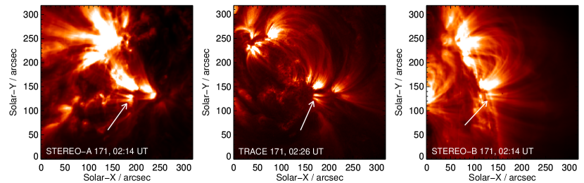
Figure 1: Images of active region AR 11032 in the 171 Å filters of the TRACE satellite (middle) and the EUVI instruments of the STEREO-A and STEREO-B spacecraft (left and right, respectively), obtained on 2009 November 22. Both STEREO images were obtained at 02:14 UT and the TRACE image was obtained at 02:26 UT. The locations of the two adjacent loop footpoints studied in the present work are indicated with an arrow in each image.

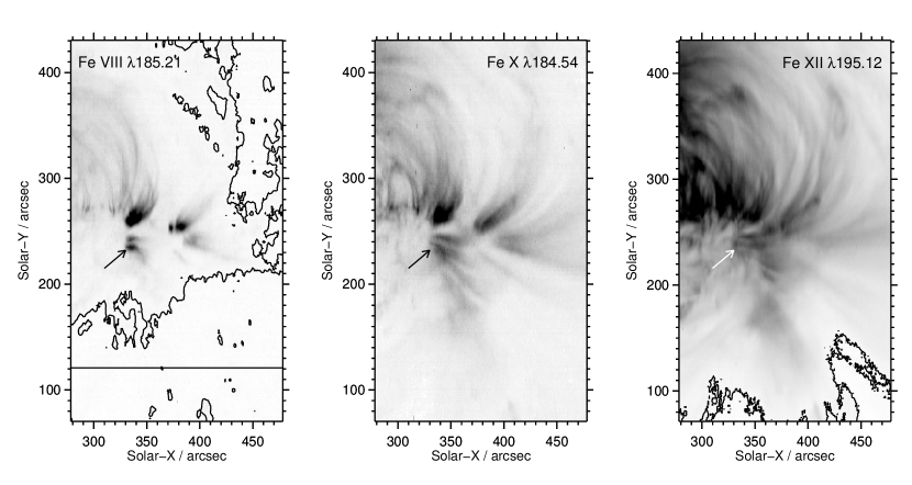
Figure 2: Images from the Fe viii $\lambda$185.21, Fe x $\lambda$184.54 and Fe xii $\lambda$195.12 emission lines derived from the EIS raster scan that began at 2009 November 21 23:44 UT and lasted 2 hours 36 mins (EIS rasters from right to left). Black corresponds to regions of high intensity, and each image has been saturated to reveal weaker emission regions. The contour in the left panel has been set at 1.5 times the average quiet Sun $\lambda$185.21 intensity, and that in the right panel is set at two times the average quiet Sun $\lambda$195.12 intensity (see text for more details). Arrows on each image point to the footpoint of the loop that is analyzed in the present work. The horizontal line on the Fe viii image marks the upper boundary of the quiet Sun region discussed in Sect. 6.1.

4 Measuring absolute velocities with EIS

To determine absolute line-of-sight velocities it is necessary to be able to compare the measured spectrum with a calibration spectrum where the lines of interest are either at rest or at a known velocity. Ideally this would be done using an on board calibration lamp that yields accurately known wavelengths. Unfortunately it is not practical to fly calibration lamps for the EIS wavelength ranges, and no flight-quality lamp exists. There are several reasons for this, including the lack of useful materials to use as the lamp window (typical materials such as quartz, LiF and MgF are all opaque below 1000 Å); large power requirements; and the weakness of the EUV spectrum from gases that might be used in the lamp (e.g., Ne, Ar).

An alternative method is to use photospheric or low chromosphere lines measured in the same spectrum as the lines of interest. These cool lines typically show only very small velocity shifts and thus can be treated as at rest, allowing the absolute wavelength scale to be determined. An example of the use of this method was provided by Brekke et al. (1997) who used emission lines from neutral and singly-ionized species such as O i, C i and Fe ii to yield an absolute wavelength scale for the SOHO/SUMER instrument. Justification for this method comes from the work of Hassler et al. (1991), who used data from a rocket-based spectrometer with an on board calibration lamp to show that an emission line of Si ii has a zero net velocity shift in the quiet Sun. Additional support for the small velocities of photospheric lines comes from the analysis of Samain (1991) who used absorption lines of Si i, Fe i and Ge i measured from a balloon experiment to determine an absolute photospheric redshift of 1 km s^-1. Although significant for the photosphere, this velocity is small compared to typical transition region and coronal velocities and means that the photospheric lines can be usefully considered to be at rest.

For the EIS wavelength ranges this method can not be used as the coolest emission line in the spectrum is He ii $\lambda$256.32 (actually a self-blend of two lines) that is formed around 80,000 K and so can not be considered a photospheric or low chromosphere line. The method of using photospheric or low chromosphere lines to set the absolute wavelength scale can thus not be applied to the EIS spectra.

Another method for determining an absolute wavelength scale is to assume that coronal lines have a zero net line-of-sight velocity above the solar limb, which is a plausible assumption given the long line-of-sight and the likelihood that the line-of-sight components of any bulk plasma motions would balance out. Two EIS exposures can then be made, one at the limb and one at the location of the active region on the disk, with the limb spectrum yielding the wavelength calibration. This method does not work however due to the orbital thermal drift effect discussed in Sect. 2, which means that the spectral position obtained at the limb will no longer be valid when the active region exposures are taken on the disk.

A further method for determining the absolute wavelength calibration is to observe quiet Sun simultaneously with the active region. That is, each individual EIS exposure will contain emission from both active region and quiet Sun at locations along the slit. The average absolute velocity of the quiet Sun as a function of temperature was accurately established by Peter & Judge (1999) using SUMER spectra. Thus, for an EIS emission line formed at a specific temperature, the quiet Sun velocity from the velocity curve shown in Fig. 6 of Peter & Judge (1999) can be obtained and used to convert the measured EIS quiet Sun velocity to a rest wavelength. This is the method used in the present work.

A potential problem for this method is the highly dynamic nature of the the quiet Sun at transition region temperatures, which means that a specific patch of quiet Sun may not show the velocity pattern found by Peter & Judge (1999). Further, quiet Sun in the vicinity of an active region may show significant differences from a quiet Sun region far from centers of activity. These issues can not be investigated with the EIS data, however we note that (i) the quiet Sun regions selected from the EIS rasters are averaged over 50″ in the Y-direction (Fig. 2) and so represent a spatial average over the quiet Sun; (ii) the error bars provided by Peter & Judge (1999) are derived from the spatial variation of the velocity shifts over the quiet Sun and are included in the present analysis; and (iii) the emission line intensities found for Fe viii in the quiet Sun region shown in Fig. 2 are consistent with an average quiet Sun value (see Sect. 6.1). We thus believe it is a reasonable approximation to apply the Peter & Judge (1999) quiet Sun velocity results to a quiet Sun location close to an active region.

An alternative means of deriving the absolute wavelength scale for EIS data has been presented by Kamio et al. (2010). Here an empirical model that relates the variation of the Fe xii $\lambda$195.12 line centroid to various temperature measurements within the EIS instrument over the entire EIS mission has been created. By assuming that Fe xii has a zero net velocity shift for all EIS exposures, the model is able to yield an absolute wavelength scale for any exposure obtained at any point in the mission. As the temperature data used by the model comes from the EIS housekeeping data-stream, this wavelength calibration method is referred to as the “HK method”. Kamio et al. (2010) give an accuracy for the HK method of 4.4 km s^-1. A comparison between the HK method and the quiet Sun method used here is presented in Appendix A, where it is seen that there is a systematic offset in the two wavelength calibrations of 5.4 km s^-1. The quiet Sun method of wavelength calibration is preferred here as it can be directly related to previous, accurate measurements of solar velocities.

Even after the absolute wavelength scale has been determined for the quiet part of the raster, the instrumental issues mentioned in Sect. 2 mean that the absolute wavelength scale can not be directly applied to the spatial locations within the active region structures. Firstly, the EIS slits are not straight nor are they exactly aligned to the axes of the detectors. This means that the rest wavelength of a line will change with the Y-location of the CCD, and so the rest wavelength determined from the quiet Sun part of the slit image needs to be adjusted in order to apply it to the active region structure. The tilts have been measured quite precisely by Kamio et al. (2010) and the parameters from this work are used here.

A second instrumental issue that affects velocity measurements appears to be due to a distorted point spread function for the EIS instrument, and this is discussed in the following section.

5 Asymmetric velocity distributions

A striking feature of velocity maps obtained from EIS is that regions of strongest redshift or blueshift are often spatially offset from regions with the highest intensity. This effect is found in the present work for the loop footpoints highlighted by an arrow in the left panel of Fig. 2 and is shown in Fig. 3. A sub-region of size 41 pixels $\times$ 41 pixels has been extracted from the full Fe viii image of Fig. 2 and Gaussian fits to the $\lambda$185.21 line have been performed at each spatial pixel to yield line intensity and centroid measurements. Absolute velocities have been derived using the method described in Sect. 6.1. The slice through the data at X-pixel 57 shows two distinct intensity peaks at Y-pixels 164 and 172, but the velocity peaks occur at Y-pixels 161 and 169, respectively. Although this feature could be explained by plasma rotating around the axes of the loops, a survey of several loop footpoints performed for this work showed that, where significant redshifts could be identified from the Fe viii line, they were always to the south of the location where the intensity peaked, no matter where the active region was located on the Sun. In addition, it is clear from inspection of high resolution TRACE images that loops that are apparently monolithic actually comprise multiple, narrow features thus a large scale twisting flow is difficult to interpret within this type of physical structure.

To state the observed effect simply, wherever there is a decreasing intensity gradient from north to south, the centroid of the emission line will be artifically shifted to longer wavelengths (redshift); and wherever there is an increasing intensity gradient from north to south, the centroid of the emission line will be artifically shifted to shorter wavelengths (blueshift). Observations of polar coronal holes provide another illustration of the effect that is apparent due to limb brightening in coronal lines. Tian et al. (2010) presented velocity maps of the north polar hole obtained with EIS where a distinctive ridge of redshifts is found along the limb in the Fe xii $\lambda$195.12 and Fe xiii $\lambda$202.04 emission lines. This arises because there is a decreasing intensity gradient from north to south at the limb. Inspection of velocity maps from the south polar hole show a ridge of blueshifts as the intensity gradient is in the opposite direction. Tian et al. (2010) also reported that the bright points within the coronal hole systematically displayed blueshifts on one side and redshifts on the other. The authors interpreted this as siphon flows within the structures but it may actually be due to the strong intensity gradients when bright points are observed within a dark coronal hole.

A similar effect was found from spectra from the Coronal Diagnostic Spectrometer (CDS; Harrison et al., 1995) instrument on board SOHO and was explained in terms of an asymmetric point spread function (PSF) by Haugan (1999). Consider a PSF in the shape of a 2-dimensional Gaussian function, but with an elliptical cross-section. The axes of the ellipse are tilted relative to the wavelength–solar-Y axes of the detector such that the long axis of the ellipse is at an angle of 135^∘ to the wavelength axis. Now if a bright spot of emission is imaged, the photon counts will appear on the detector as an ellipse. On the north side of the ellipse, there is an excess of counts to the short wavelength side of the spot, while on the south side of the ellipse there is an excess of counts on the long wavelength side of the spot. Measuring the centroid of the spot as a function of solar-Y will thus show a blueshift on the north side of the spot, and a redshift on the south side, consistent with the pattern shown in Fig. 3. Note that if the PSF was rotated through 90^∘ then the opposite velocity pattern would appear in the observations.

The PSF will be expected to vary with position along the 1024″ length of the EIS slit due to optical properties of the spectrometer, therefore the pattern of redshifts and blueshifts induced by the PSF would be expected to change, but this is beyond the scope of the present work. If the above interpretation of the data is correct, then the simplest way of deriving velocity shifts for features with steep intensity gradients is either to study only those pixels at the location of the intensity peaks in the solar-Y direction, or to perform averaging in the Y-direction over a region symmetrically distributed around the intensity peak. This is the procedure employed in the present work.

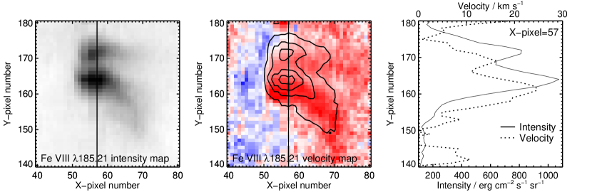
Figure 3: The left panel shows the Fe viii $\lambda$185.21 intensity map in the vicinity of the loop footpoints. The middle panel shows the $\lambda$185.21 velocity map of the same location with velocities between $\pm$ 25 km s^-1 displayed, and the contours of the intensity map overplotted. The right panel shows cuts through the intensity and velocity maps at X-pixel 57, which is indicated on the left and middle panels with a vertical, solid line. The solid and dashed lines in the right panel show intensity and velocity, respectively. Interpolation has been peformed for missing data at X-pixels 47, 54 and 55.

6 Velocity derivation method

In this section we describe the particular steps involved in deriving the absolute velocities and associated uncertainties for the 2009 November 21 data-set. As described in Sect. 4, the method requires a determination of the rest wavelength scale from a patch of quiet Sun that is observed simultaneously with the active region. Ideally the strongest line in the spectrum should be used for this in order to give the best possible measurement in the quiet Sun. However the strongest EIS lines from the quiet Sun are all formed at temperatures of 1–2 MK, the temperature range where the active region has its largest spatial extent. This is illustrated in the right panel of Fig. 2 which shows the raster image obtained in Fe xii $\lambda$195.12, the strongest line observed by EIS (formed at 1.5 MK). Bright loop structures are clearly seen to extend all the way to the top of the raster and, although the bottom of the raster appears to be dark (and thus potentially classed as quiet Sun), the intensity is still significantly brighter than average quiet Sun levels. This is indicated by the black contour which shows locations where the $\lambda$195.12 intensity is a factor 2 brighter than the average quiet Sun value measured by Brooks et al. (2009). At no point in the $\lambda$195.12 image does the intensity fall to average quiet Sun levels.

The Fe viii $\lambda$185.21 image shown in the left panel of Fig. 2 shows that the active region has a significantly smaller spatial extent at cooler temperatures. The contour, which in this case is set at 1.5 times the quiet Sun $\lambda$185.21 intensity measured by Brooks et al. (2009), shows that a significant fraction of the image at the bottom of the raster can be considered to be quiet Sun. For this reason we choose to use Fe viii $\lambda$185.21 as the line from which the rest wavelength scale is determined in the present work.

Fe viii represents the ideal ion to use for the EIS wavelength calibration as (i) it is sufficiently strong that it can be measured accurately in the quiet Sun, and (ii) the active region has a relatively small spatial extent in this ion. Emission lines from cooler ions in the EIS wavelength ranges, such as O vi $\lambda$184.11 and Mg vi $\lambda$268.99, are too weak to be reliably measured in the quiet Sun, while the active region is too extended in images from the hotter coronal ions (Fe x–xiii) to enable the quiet Sun to be seen within the EIS field of view. The isolated Fe ix $\lambda$197.86 line (first identified by Young, 2009) is possibly an alternative to Fe viii but was not measured in the present data-set. Si vii $\lambda$275.37 is formed at a similar temperature to Fe viii $\lambda$185.21 (Table 1) but is a factor two weaker and so not as easily measured in the quiet Sun. $\lambda$186.60 and $\lambda$194.66 are two other Fe viii lines that could have been used as references since their signal-to-noise is comparable to $\lambda$185.21 (Young et al., 2007b; Brown et al., 2008). However, $\lambda$186.60 was not observed in the 2009 November 21 raster while $\lambda$194.66 is partially blended with a line in the long wavelength wing and so is less suitable than $\lambda$185.21 for velocity measurements.

Fe viii $\lambda$185.21 is used to determine a rest wavelength from the quiet Sun and the detailed method for doing this is described in Sect. 6.1. For other lines it is necessary to calibrate relative to $\lambda$185.21 by making use of standard wavelength separations that are measured from the EIS spectra. Different methods are required for the two EIS wavelength channels and these are described in Sects. 6.2 and 6.3, respectively.

6.1 Velocities from Fe VIII $\lambda$185.21

The first step is to fit the Fe viii $\lambda$185.21 line in the quiet Sun region at the bottom of the raster (see the left panel of Fig. 2). The bottom 50 Y-pixels of the raster image are selected and the data are binned in the Y-direction over this 50 pixel region, then Gaussian fits performed to each of the 200 pixels in the X-direction. Binning is required to give sufficient signal in the $\lambda$185.21 line to allow the line centroid to be measured accurately; it also ensures that any local inhomogeneities in the quiet Sun are smoothed over. The $\lambda$185.21 intensity over the 200 X-pixels is shown in the upper panel of Fig. 4 where the level is mostly below the average quiet Sun intensity found by Brooks et al. (2009). We note that the EIS sensitivity has probably decreased between the present observation and that of Brooks et al. (2009), which was obtained on 2007 January 30. Preliminary measurements of the sensitivity decay (J.T. Mariska, 2011, private communication) suggest an exponential decay with a 1/e time of 1894 days. This would imply that the EIS sensitivity has decreased by a factor 0.58 between the two observations. The dash-dot line in Fig. 4 shows the Brooks et al. (2009) quiet Sun measurement multiplied by 0.58, placing it in good agreement with the intensities measured in the quiet part of the Fe viii raster. This confirms that the quiet region considered here can be reasonably classed as quiet Sun. The bottom panel of Fig. 4 shows the variation of the $\lambda$185.21 centroid over the quiet Sun region. The oscillatory pattern reveals the orbital thermal drift described in Sect. 2. A spline fit to the $\lambda$185.21 centroid variation is then performed, with the spline defined at 10 minute nodes (recall that each X-pixel represents a different point in time due to the nature of the EIS observations; 10 mins corresponds to around 13 X-pixels for this data-set). The standard deviation of the difference between the actual centroid measurements and the fit is 2.1 mÅ. This is the uncertainty in the quiet Sun wavelength scale, denoted by $\sigma_{\rm qs}$, which is used in the error analysis later.

Figure 4: The upper panel shows the variation of the Fe viii $\lambda$185.21 emission line intensity in the quiet Sun band of the 2009 November 21 raster. The intensity at each position is derived from an average of 50 spatial pixels in the solar-Y direction. The dashed line denotes the average quiet Sun intensity of Fe viii $\lambda$185.21 found by Brooks et al. (2009), and the dash-dot line shows this value multiplied by 0.58 (see main text for more details). The lower panel shows the measured $\lambda$185.21 line centroids at each of the quiet Sun pixels, demonstrating the orbital variation of line position. The thick solid line shows the spline fit to the centroids.

Fe viii $\lambda$185.21 will not be at rest in the quiet Sun and it is necessary to determine the average quiet Sun velocity using the velocity curve provided by Peter & Judge (1999). This is done by finding which of the ions used by Peter & Judge (1999) is closest in temperature to Fe viii. Table 1 gives a $T_{\rm eff}$ value of 5.85 which fortuitously matches the value for Ne viii $\lambda$770.41, one of the lines used by Peter & Judge (1999). The average velocity shift for this line is $v_{\rm PJ}=-2.6\pm 1.8$ km s^-1 (blueshift), and therefore we assume this applies to Fe viii $\lambda$185.21. If we take the measured quiet Sun wavelength of $\lambda$185.21 as determining the rest wavelength at Y-pixel $q$, the center of the chosen quiet Sun region (pixel 25 in the present case), then the rest wavelength for a X-pixel $i$ is:

$$\lambda_{\rm rest}(i,q)=\lambda_{\rm qs}(i,q)-{v_{\rm PJ}\over c}\lambda_{\rm qs}(i,q)\cos\,\theta$$ (3)

where $\lambda_{\rm qs}$ is the wavelength from the spline fit shown in the bottom panel of Fig. 4, $c$ is the speed of light, and $\theta$ is the heliocentric angle ($\theta=0$ is disk center). For the region considered here, $\cos\,\theta=0.90$–0.93 and, for simplicity, we take a value of 0.92 at all spatial pixels in the raster. The rest wavelength will change with Y position due to the EIS slit tilt such that

$$\lambda_{\rm rest}(i,j)=\lambda_{\rm rest}(i,q)+t(j)-t(q)$$ (4)

The EIS slit tilts, $t(j)$, are described by cubic polynomials and the coefficients are given by Kamio et al. (2010).

If we consider a pixel $(i,j)$ within the active region loop, then we now have the rest wavelength at this pixel position against which the loop velocity can be determined. Since velocities at individual pixels are affected by the point spread function problem (Sect. 5), however, then we choose for the present study to average spectra from the loop over Y-regions that span the loop cross-section; the asymmetries then cancel out to yield more accurate velocities. The Y-regions selected for each X-pixel location are discussed in Sect. 7. The measured loop velocities thus correspond to pixels $(i,p_{i})$ where $p_{i}$ is the Y-pixel corresponding to the center of the chosen loop Y-region at each X-pixel $i$.

The error on the absolute velocity for Fe viii $\lambda$185.21 comprises four components that are added in quadrature:

$$\sigma_{\lambda}^{2}=\sigma_{\rm loop}^{2}+\sigma_{\rm tilt}^{2}+\sigma_{\rm qs}^{2}+\sigma_{\rm PJ}^{2}$$ (5)

where $\sigma_{\rm loop}$ is the measurement error of the emission line wavelength in the loop, $\sigma_{\rm tilt}$ is the uncertainty in the determination of the slit tilt parameters, $\sigma_{\rm qs}$ is the uncertainty in the determination of the orbit variation, and $\sigma_{\rm PJ}$ is the uncertainty in the absolute velocity of Fe viii $\lambda$185.21 in the quiet Sun as obtained from Peter & Judge (1999). For the present case the dominant error term is $\sigma_{\rm qs}$ which is 2.1 mÅ; $\sigma_{\rm PJ}$ is 1.1 mÅ, $\sigma_{\rm tilt}$ is between 0.1 and 0.2 mÅ, and $\sigma_{\rm loop}$ varies from 0.4 mÅ to 1.4 mÅ depending on the signal in the loop line profile. Note that $\sigma_{\rm loop}$ and $\sigma_{\rm qs}$ are random errors, whereas $\sigma_{\rm tilt}$ and $\sigma_{\rm PJ}$ are systematic errors. The combined errors lead to absolute velocity uncertainties of 4–5 km s^-1 for Fe viii $\lambda$185.21.

6.2 Velocities for other SW lines

For other emission lines within the EIS SW band, the above limb wavelength offsets of Warren et al. (2011) are used: the Fe viii $\lambda$185.21 rest wavelength at loop position $(i,p_{i})$ sets the absolute wavelength scale and the rest wavelengths of other lines are obtained from the wavelength offsets relative to $\lambda$185.21 given in Table 1 of Warren et al. (2011). The wavelength offsets have uncertainties, $\sigma_{\rm limb}$, that are obtained from Warren et al. (2011) by combining in quadrature the error for the line of interest with that of $\lambda$185.21. Warren et al. (2011) did not include O vi $\lambda$184.11 although this line can be seen in off-limb spectra. Using the same data-set as Warren et al. (2011) we find a wavelength of $184.1161\pm 0.0005$ Å.

6.3 Velocities in the LW band

Potentially the method of using off-limb wavelength offsets can be extended to the EIS LW band. However, studying a number of quiet Sun data-sets it is apparent that the offset of Si vii $\lambda$275.35 relative to $\lambda$185.21 shows variations of up to 0.02 Å over long time-scales. The procedure for checking this was to consider quiet Sun rasters and measure the Fe viii and Si vii lines in “macro-pixels” of size 2$\times$20 pixels (for example) that are chosen to yield strong enough signals for measuring line centroids accurately. Constructing histograms of the wavelength differences between the lines across the raster yields a Gaussian-shaped curve with a full-width at half maximum of around 2–3 mÅ. However, the centroid of the Gaussian distribution varies from 90.16 to 90.18 Å. The small dispersion in the measured separations is consistent with the two emission lines having the same $T_{\rm eff}$ value (Table 1), but the longer time-scale variation is a surprise and suggests that slow thermal effects within the instrument may cause the wavelength scale to stretch or shrink over time. The changes are small for lines within the SW band due to the small wavelength separations, but become significant when comparing SW to LW separations. The end result is that SW–LW separations from an off-limb data-set such as that analyzed by Warren et al. (2011) can not be applied to a data-set taken at a different time.

An alternative is to treat the LW channel independently, and measure Si vii $\lambda$275.37 in the quiet Sun part of the active region raster in the same manner as was done for Fe viii $\lambda$185.21 However, $\lambda$275.37 is around a factor two weaker than Fe viii $\lambda$185.21 and, coupled with the fact that around 18 of 50 quiet Sun pixels are lost because of the offset between the two EIS CCDs (Sect. 2), the $\lambda$275.37 signal in the quiet Sun region is insufficient to reliably obtain the orbit variation.

The solution for the present work is to assume that the velocity shift of Si vii $\lambda$275.37 at a specified spatial location in the loop is the same as that of Fe viii $\lambda$185.21. This is suggested by the fact that the images in the two lines are so similar, and the assumption can be checked using the present data-set.

If the two lines do show the same velocity shift, then if we create a histogram of the difference in measured wavelength between the two lines, we would expect to see only a small scatter. The two lines are normally too weak to extract reliable centroid measurements in individual spatial pixels, but they become sufficiently bright in the loop footpoints that this is possible. We filter out all spatial pixels in the November 21 raster that have a Si vii $\lambda$275.35 intensity above 300 erg cm^-2 s^-1 sr^-1 (437 in all). We then remove those pixels for which $\lambda$185.21 is not reliably measured, giving 432 pixels. (Note that a CCD spatial offset of 18 pixels between the two emission lines needs to be accounted for when doing this comparison.) For these 432 pixels, Fig. 5 shows the distribution of wavelength separations. The mean separation is 90.1841 Å, but more importantly the standard deviation is only 0.0020 Å, corresponding to a velocity shift of 2.1 km s^-1. Part of this dispersion will be due to the different slit tilts that apply to the two wavebands. All of the selected spatial pixels lie within a 50 pixel band in the Y-direction, over which the slit tilt difference changes by only 1 mÅ, so this is only a minor contribution. The small dispersion in the $\lambda$275.37–$\lambda$185.21 wavelength separation gives confidence that the Si vii $\lambda$275.37 velocity shifts mimic those of Fe viii $\lambda$185.21, and so supports our assumption that $\lambda$275.37 has the same velocity shift as $\lambda$185.21.

The rest wavelength of $\lambda$275.37 within the loop is thus obtained by taking the measured $\lambda$185.21 loop velocity and correcting the measured $\lambda$275.37 wavelength in the loop by this velocity. For example, suppose $\lambda$185.21 has a blueshift of $15$ km s^-1 in the loop and, at the same spatial location, the measured wavelength of Si vii $\lambda$275.37 is 275.355 Å. The Si vii line is assumed to have the same velocity shift as the Fe viii line, so adding a shift of +15 km s^-1 to the measured Si vii $\lambda$275.37 wavelength yields the rest wavelength of 275.369 Å. An additional error component of 0.0020 Å is added in quadrature to the $\lambda$185.21 error components (Eq. 5) to account for the dispersion in Fig. 5.

For other lines in the LW channel the off-limb wavelength offsets of Warren et al. (2011) can be used to yield the rest wavelengths from the $\lambda$275.37 rest wavelength. However, our primary interest in the LW channel for the present work is to give access to the cool emission lines O iv $\lambda$279.93 and Mg vi $\lambda$268.99 that can not be reliably measured in off-limb spectra. The O iv line is particularly interesting as it is predicted to be formed at 180,000 K in the quiet Sun (Table 1) and represents the coolest emission line that can be used for velocity measurements with EIS.

The procedure for determining rest wavelengths for O iv and Mg vi from the $\lambda$275.37 line is as follows: all three lines were measured in a set of eight average quiet Sun spectra obtained with EIS in 2007 (six spectra), 2009 and 2010 (one spectrum each). The spectra were averaged over a sufficiently large spatial region to yield good measurements of the line centroids. The separations of the lines were computed, and an average taken. An error on the separation was taken from the standard deviation of the different quiet Sun measurements. The offsets relative to $\lambda$275.37 are found to be $4.5724\pm 0.0025$ Å and $-6.3816\pm 0.0012$ Å for O iv $\lambda$279.93 and Mg vi $\lambda$268.99, respectively. Now these offsets apply to the quiet Sun, which has its own velocity structure. Therefore the separations need to be corrected for the average quiet Sun velocities of Peter & Judge (1999) to yield the rest wavelength separations. O iv was measured by Peter & Judge (1999) in the quiet Sun and was found to have a velocity shift of $+9.9\pm 2.7$ km s^-1. Mg vi was not measured by Peter & Judge (1999), but from the CHIANTI atomic data we find that it is expected to be formed at $\log\,T=5.7$ in the quiet Sun placing it between O vi and Ne viii, which were measured by Peter & Judge (1999). We assign Mg vi a quiet Sun velocity of $0.0\pm 2.0$ km s^-1. For Si vii, we assume it has the same quiet Sun velocity as Fe viii and Ne viii.

The rest wavelength separations of O iv to Si vii, and Mg vi to Si vii are thus $4.5607\pm 0.0039$ Å and $-6.3840\pm 0.0027$ Å, respectively. These values are used to determine the O iv and Mg vi rest wavelengths from the Si vii rest wavelength.

Figure 5: Histogram showing the wavelength separations of the Si vii $\lambda$275.37 and Fe viii $\lambda$185.21 lines over 432 pixels in the loop footpoint regions of AR 11032.

7 Large-scale velocity structure

Figures 1 (middle panel) and 2 identify two nearby loop footpoints in AR 11032 that are well defined in the TRACE 171 channel and EIS Fe viii $\lambda$185.21. The aim of the present work is to measure the line-of-sight velocities along one of these loops from ion emission lines formed at different temperatures. For this it is necessary to have confidence that the loop is well-defined at each temperature considered. For ions formed at temperatures similar to Fe viii or below (see Table 1) this is straightforward as the images formed in these ions show the same pair of compact brightenings that the Fe viii image shows. For higher temperatures the loop identification becomes more difficult.

The four upper panels of Fig. 6 show intensity images from the lines Fe viii $\lambda$185.21, Fe x $\lambda$184.54, Fe xi $\lambda$188.22 and Fe xii $\lambda$195.12 for a 61 pixel $\times$ 61 pixel sub-region of the full EIS raster that shows the footpoint region. The two distinct footpoints are clearly seen in the Fe viii $\lambda$185.21 image where they are labeled ‘N’ and ‘S’ for north and south, respectively. The Fe x $\lambda$184.54 image shows much more extended structures, and two loops labeled ‘A’ and ‘B’ can be matched with the two footpoints N and S. There are two additional patches of enhanced emission labeled ‘C’ and ‘D’ that may be loops that connect to footpoint S. The higher spatial resolution of the TRACE 171 channel images can be used to study the morphology of the EIS Fe x image in more detail as the principal component to the channel’s response comes from Fe x. The four lower panels of Fig. 6 show TRACE 171 images obtained at four times during the course of the EIS raster. The times at which the TRACE images were taken are indicated by four short vertical lines at the top of the EIS Fe x image. The TRACE images show that the basic morphology of the loops remains the same during the EIS raster. Footpoint S appears to have two narrow, nearby loops associated with it, although these are not resolved in the EIS data. The upper of these narrow loops appears to connect to the solar surface between S and N at the early part of the raster, but is closer to S when EIS rasters the footpoint. The upper loop structure A is clearly separated from B and connects to footpoint N. In the TRACE images, the structures C and D do not connect to footpoint S.

Loop A is more distinct than loop B, however the key Fe viii $\lambda$185.21 line is affected by missing pixels in the center of the line profile that would affect velocity determinations. We therefore focus on loop B and the footpoint S, which are identified by a pair of black lines in each of the upper panels of Fig. 6 that were drawn based on a study of the EIS Fe viii and Fe x images, and the TRACE 171 images. Since the TRACE 171 images show that loop B consists of two distinct strands then we will generally refer to it as “loop structure B” to denote that it is not a single monolithic structure. Indeed the discussion presented in the following paragraphs suggests there is additional structure to that seen in the TRACE 171 images. The common feature of the individual strands within loop structure B is that they appear to terminate in footpoint S.

Moving to the hotter Fe xi $\lambda$188.22 line, the structures A–D become brighter away from the footpoint region but also the emission, in general, becomes more diffuse over the raster. Considering structure B there appears to be two brightness components: one that spatially matches the bright region of Fe x (around X-pixels 55–70), and another that extends to larger heights (X-pixels 70–90). The two components are seen more clearly in the Fe xii $\lambda$195.12 image where there is a definite gap between the extended emission around X-pixels 75–100 and the Fe x brightness patch around X-pixels 55–70. In general, the Fe xii image shows little relation to the very simple two footpoint image of Fe viii and thus hints at increasing complexity with height/temperature.

Our interpretation of the image data is that there are many loops coming from the both the Fe viii bright footpoints (N and S) and other footpoints that are not bright in Fe viii (e.g., the invisible footpoints of structures C and D). These loops have a range of angles to the solar surface, perhaps related to where the loops connect back to the solar surface on the opposite side of the active region (see below). For low temperatures/height (Fe viii) the different loops converge and give the impression of distinct, bright patches of emission. For larger temperatures/height (Fe xii) the loops diverge from each other and give much less distinct emission signatures. In particular, the Fe x brightness patch of loop B that is seen in both Fe xi and Fe xii is likely a distinct structure from the extended, diffuse emission seen in Fe xi and Fe xii over X-pixels 75–100, even though both have their footpoints within footpoint S of Fe viii.

Evidence for the different connectivity of loops coming from footpoints N and S is provided from the STEREO data. The EUVI instruments of the STEREO A and B spacecraft obtained 195 Å filter images at a cadence of 2.5 and 5 min, respectively, during the course of the EIS raster. The image frames from 01:30:30 UT, when EIS was rastering across the footpoint regions, are shown in Fig. 7. Compared to the TRACE 171 Å filter images shown in Fig. 1, the active region loops can be seen to extend to greater heights and the footpoint region considered here is found to connect to two distinct parts of the active region. The direction of the two groups of loops are indicated by pairs of red lines overlaid on the Fig. 7 images. The northerly group of loops connects to a bright part of the active region, whereas the more southerly loops connect to a fainter part of the active region. We may speculate that the Fe x brightness patch discussed above belongs to the lower group of loops, whereas the Fe xi–Fe xii extended structure belongs to the upper group of loops.

The above discussion shows that relating Fe xii emission structures to Fe viii structures is very difficult and, certainly in the present case, not unambiguous. The principal velocity result from this work relates to Fe viii and Fe x for which the relation between emission structures is very clear (Fig. 6). However, the velocity derived from Fe xii is also of interest due to the presence of an active region outflow region very close to the Fe viii footpoints. This will be discussed in Sect. 10 where further analysis of the morphology of the Fe xii structures will be given.

The following section will present velocities for loop structure B that are averaged across the loop’s diameter, and Sect. 9 will present density and filling factor estimates for the loop.

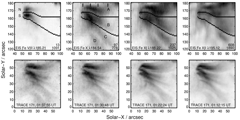
Figure 6: The upper four panels show the loop footpoint region in four emission lines observed by EIS, which scanned from right to left between 01:01 and 01:48 UT on 2009 November 22. The four lower panels show the same footpoint region observed in the TRACE 171 filter at four different times during the EIS raster. The EIS spatial locations corresponding to these times are indicated by the thick, black lines near the top of the EIS Fe x image. The two black lines in each of the EIS images identify the loop structure analyzed in the present work. The numbers in the bottom right of each EIS image give the minimum (upper) and maximum (lower) intensity values (units: erg cm^-2 s^-1 sr^-1) in each image. A linear, inverse scaling is used for all images, with black indicating regions of high intensity. The X and Y-axes for the EIS images are relative to the bottom-left corner of the complete EIS raster; those for the TRACE image are relative to the bottom-left corner of the displayed images.

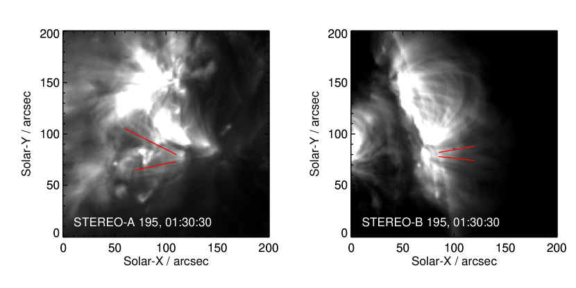
Figure 7: STEREO/EUVI 195 Å filter images from the A and B spacecraft (left and right panels, respectively) obtained on 2009 November 22 01:30:30 UT. Red lines indicate the approximate direction of the two groups of loops that emanate from the footpoint region studied in the present work.

8 Loop structure B

Fig. 6 shows the region used to define the loop structure B. The spectra along the data columns between (and including) the two black lines are summed in the Y direction, leading to a single 1D spectrum for each X-position along the loop. The summation is necessary both to improve signal-to-noise in weak lines and to correct any distortions to the line centroid position caused by the potentially distorted PSF of EIS (Sect. 5). Spectra at each X-position along the loop were created using the Solarsoft IDL routine EIS_MASK_SPECTRUM which averages the signal from each spatial pixel in the loop cross-section. The emission lines in the resulting 1D spectra were then fit with Gaussian profiles using the Solarsoft routine SPEC_GAUSS_EIS to yield intensity, velocity and line width values for each line. In total, 43 spectra corresponding to X-pixels 51 to 95 (pixels 54 and 55 were missing) were fit. In general we will refer to the X-direction as representing the “height” along the loop, with pixel 51 being the bottom of the loop.

Fig. 8 shows the intensity variation along loop structure B for nine different emission lines observed by EIS. For the lines formed at temperatures $\log\,T_{\rm eff}\leq 6.05$ (Table 1) there is a clear correlation between the height at which the intensity peaks and the temperature. The two coolest ions, O iv and O vi, both peak at the lowest height and Mg vi peaks two pixels higher up the loop. Fe viii, Si vii and Mg vii each peak around the same position, three to five pixels higher than Mg vi, which is consistent with their $T_{\rm eff}$ values. The trend continues with Fe x $\lambda$184.54 which has a broad peak several pixels higher than Fe viii.

The intensity profiles for Fe xi and Fe xii are more complex, each showing two peaks of enhanced emission along the loop. Both peak in intensity at a location that is a good match to that where Fe x is most enhanced (X-pixels 58 to 66). The second peak for Fe xi is around X-pixel 75, and that for Fe xii is around X-pixel 83. As discussed in the previous section, our interpretation is that the two intensity peaks of Fe xi and Fe xii probably represent two groups of loops that head towards different parts of the active region, even though they both originate from footpoint S. The cooler ions (Fe x and below) are principally formed at lower heights where there is less distinction between the two groups of loops and so a more simple dependence of line intensity with height is found.

The velocities along loop structure B are presented in Fig. 9 which shows the velocities from five emission lines within the EIS SW band, displayed over two panels for greater clarity. The key result is that Fe viii, over the pixel range 56 to 68, displays a significant redshift of around 15 km s^-1, yet Fe x in the same spatial location is close to rest (there is a trend of increasing redshift with height from $-5$ to $+3$ km s^-1). Taking into account the error bars, the Fe x velocity is almost consistent with being at rest. The cooler O vi $\lambda$184.11 line can only be measured accurately in the lowest heights of the loop structure, but shows values consistent with Fe viii. Fe xi and Fe xii show very similar behaviour, with each being close to rest at X-pixels 70 and above, but showing significant blueshifts in the lower heights of the loop structure (X-pixels 51–65). Fe x also displays significant blueshifts at the lowest heights. Our interpretation of these blueshifts is that they arise from an “outflow region” (e.g., Harra et al., 2008; Doschek et al., 2008; Bryans et al., 2010) for which the plasma intrudes into the line of sight of loop structure B. This is discussed in Sect. 10.

The EIS LW spectrum gives access to additional low temperature lines and, in particular, access to O iv $\lambda$279.94 which is the lowest temperature line observed by EIS that is suitable for velocity measurements. As discussed earlier in Sect. 6.1, the use of Fe viii $\lambda$185.21 as a reference line for the wavelength calibration fails for the LW band, as the separation between the SW and LW bands varies with time. Using the method described in Sect. 6.3, the velocities derived for Mg vi $\lambda$268.99 and O iv $\lambda$279.94 are shown in Fig. 10. The Mg vi line shows good agreement with Fe viii, except for the lowest three heights where the Mg vi velocity is significantly higher. By contrast, the O iv line agrees with Fe viii at the two lowest heights, but is significantly discrepant at the third height. Considering the four coolest ions together, a definitive statement on the velocity profile at the lowest heights in the loop structure can not be made. O iv, O vi and Fe viii all suggest that the velocity decreases towards the base, whereas Mg vi suggests it remains constant, or slightly increasing. There is, however, no evidence for a significant increase in velocity towards the lower, cooler part of the loop footpoint region, i.e., a step increase in velocity occurs between Fe x ($\log\,T=6.05$) and Fe viii ($\log\,T=5.85$), but there is no further large velocity increase between $\log\,T=5.2$ and $\log\,T=5.8$.

Returning to the difference in velocities between Fe viii and Fe x, an important point to note is that it occurs at the same spatial locations and is consistently different over a 13 pixel region. One possible interpretation is that there could be two plasma components: one that is redshifted (downflowing) that emits in both Fe viii and Fe x, and one that is hotter with little Fe viii emission that is at rest or blueshifted. In this scenario Fe viii is redshifted – as observed – while the composite line profile from the two plasma components in Fe x would be significantly less red-shifted, or at rest. This can be ruled out, however, by considering the emission line widths along loop B shown in Figure 11. The measured full widths at half-maximum have been corrected for the instrumental width, as given by the Solarsoft routine EIS_SLIT_WIDTH (see also Young, 2011d), and the thermal width for which the $T_{\rm eff}$ values from Table 1 have been used. The displayed widths therefore represent non-thermal broadening. Over the X-pixel region 56 to 68, where there is a 15 km s^-1 difference between the Fe viii and Fe x velocities, the Fe x line actually displays a smaller non-thermal broadening than the Fe viii line, which is evidence against the Fe x emitting plasma having two velocity components. We therefore believe that there is no significant Fe x emitting plasma that is downflowing at speeds of 15 km s^-1.

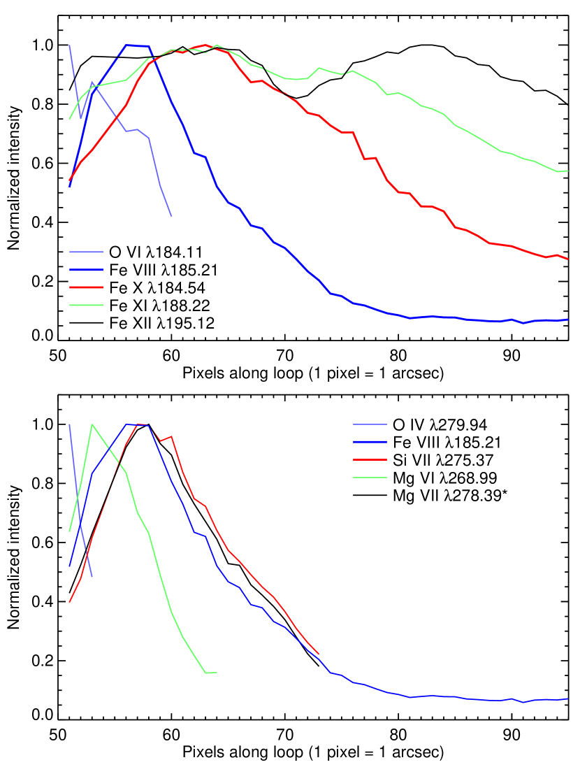
Figure 8: A comparison of intensity profiles along loop structure B (shown in Fig. 6) for selected emission lines from the EIS SW (upper panel) and LW (lower panel) channels. The Fe viii $\lambda$185.21 profile is shown in the lower panel for reference. All intensities are normalized to the maximum intensity along the loop. The Mg vii $\lambda$278.39 line intensity has not been corrected for a blend with the weaker Si vii $\lambda$278.44 line.

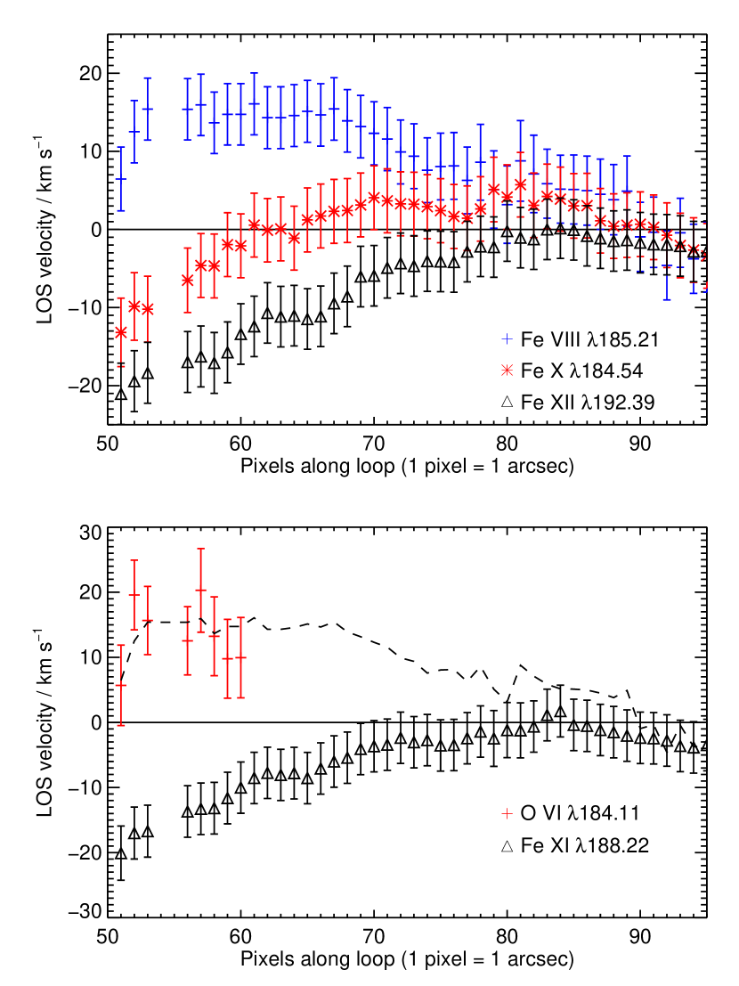
Figure 9: A comparison of the velocity profiles of five different emission lines along loop structure B (shown in Fig. 6). Note the slightly different Y-axis scales for each. In the lower panel, the Fe viii $\lambda$185.21 velocities are represented by a dashed line.

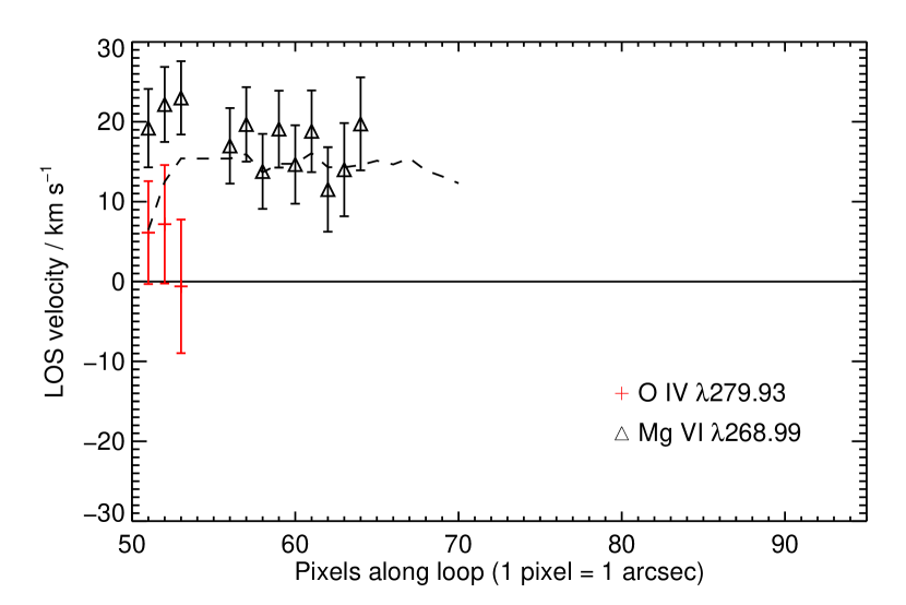
Figure 10: A comparison of the velocity profiles of the EIS LW lines O iv $\lambda$279.94 and Mg vi $\lambda$268.99 along loop structure B (shown in Fig. 6). The Fe viii $\lambda$185.21 velocities are represented by a dashed line.

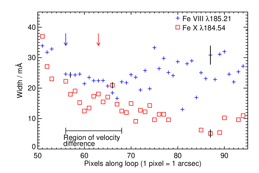
Figure 11: Non-thermal line widths of Fe viii $\lambda$185.21 (blue) and Fe x $\lambda$184.54 (red) along the loop. Error bars on selected points are indicated by vertical black lines. The downward-pointing arrows indicate the locations of the peak intensities of the two lines. The spatial region where there is a significant velocity difference between the two ion lines is indicated. Note that some data-points are missing for Fe x $\lambda$184.54 as the measured width was smaller than the combined instrumental width and thermal width at these points.

9 Density and filling factor

The velocity results for Fe viii and Fe x imply that there are multiple, independent components to the loop structure. An alternative method of studying this is to measure the loop filling factor with a density diagnostic. Mg vii is formed at a similar temperature to Fe viii and it has an excellent density diagnostic: $\lambda$280.72/$\lambda$278.39. It has previously been used for density and filling factor measurements by Young et al. (2007a), Tripathi et al. (2009) and Tripathi et al. (2010).

The filling factor at each X-pixel along the loop is determined as follows. The emission line intensities measured at each location represent the average intensities over the Y-cross-section. Following the notation of Tripathi et al. (2010), the average intensity, $I_{\rm obs}$, can be converted to a plasma column depth, $h$, with the expression

$$h={I_{\rm obs}\over 0.83A(z)G_{0}(N_{\rm e})N_{\rm e}^{2}}$$ (6)

where the constant 0.83 is the proton-to-electron ratio in the corona, $A(z)$ is the abundance of the emitting element relative to hydrogen, $G_{0}$ contains a number of atomic parameters (as described in Tripathi et al., 2010) and is a weakly-varying function of density, and $N_{\rm e}$ is the electron number density.

From the measured Mg vii line intensities along the loop, the value of $N_{\rm e}$ at each X-pixel was determined using atomic data from the CHIANTI atomic database. A background component to each intensity was estimated by considering a small region adjacent to the loop, and this was subtracted from the loop intensities. The derived densities are shown in Fig. 12 (left panel) where a general trend of decreasing density with height is seen. Using Eq. 6 the column depth at each position can be calculated. For the magnesium abundance we use the coronal value of Feldman et al. (1992), and the atomic parameter $G_{0}$ is computed from atomic data in version 6 of the CHIANTI database (Dere et al., 2009), including the ionization fractions presented in that paper. The column depths are presented in the middle panel of Fig. 12, where the size of the Y cross-section at each location is also shown.

To determine a filling factor it is necessary to make some assumption of the loop geometry. Since the loop is considered to be at an angle of $\approx 20^{\circ}$ to the line of sight, then the Y-slices at each X-pixel will be approximately elliptical with the minor diameter, $d_{i}$, given by the width of the loop in the Y direction. Assuming a loop angle of $\approx 20^{\circ}$ then implies the major diameter (in the line-of-sight) is $d_{i}/0.34$. The filling factor at X-pixel $i$ is then given by

$$f_{i}={d_{i}h_{i}\over\pi(d_{i}/2)^{2}/0.34}={1.36h_{i}\over\pi d_{i}}$$ (7)

The values of $f_{i}$ are shown in the right panel of Fig. 12.

In both the middle and right panels of Fig.12 the pixel region 53–64 is highlighted as this is where the Fe viii line intensity is strongest (Fig. 8). The method used to determine the column depth essentially requires the emission lines to be principally formed close to the temperature of maximum ionization ($T_{\rm max}$). The loop images suggest that the temperature is increasing with height along the loop, and so the Mg vii (and thus Fe viii) lines will be brightest where the loop temperature is close to the ions’ $T_{\rm max}$ values. The column depth and filling factor values should thus be most accurate in this region, and be less accurate at lower and higher heights where the displayed values are likely to be underestimates.

Another factor that strongly affects the column depth and filling factor results is the element abundance. The Feldman et al. (1992) value for Mg is a factor four larger than the photospheric value, a standard enhancement that has been reported from remote sensing observations of the corona and in situ measurements of the solar wind (Feldman & Laming, 2000). However, fan loop structures have been found to display different enhancements. Young & Mason (1997) found a factor 10 enhancement for a loop structure that was likely a fan loop, while Widing & Feldman (2001) found that the magnesium enhancement was found to increase with time in fan loop structures over several days rising to a factor 9 in one case. We thus note that a larger enhancement of Mg than that of Feldman et al. (1992) would reduce the column depth and filling factor values shown in Fig. 12.

The Mg vii filling factor increases with height, with a value of 0.05 near the base (X-pixels 51–53), and rising to around 0.3 around X-pixel 70. The spatial region where Fe viii and Fe x have different velocities has a filling factor of 0.1–0.3 at the temperature that Fe viii is formed. This is consistent with the Fe viii emitting structure only occupying a fraction of the emitting volume, with the Fe x emitting structure occupying some remaining part of the volume.

Figure 12: Electron densities, column depths and filling factors (left, middle and right panels, respectively) as a function of position along the loop derived from the Mg vii $\lambda$$\lambda$278.39, 280.72 line pair. The boxes in the middle panel show the observed width of the loop as shown in the upper panels of Fig. 6. The pixel region 53–64, where Mg vii is most intense, is highlighted in the middle and right panels.

Loop filling factors from the EIS Mg vii $\lambda$280.72/$\lambda$278.39 ratio have previously been presented by Young et al. (2007a) and Tripathi et al. (2009) who both found filling factors close to 1 in the regions close to the loops’ footpoints. The present loop structure B is known to have filamentary structure based on the two strands identified from the TRACE 171 images (Sect. 7), and so smaller filling factors are not surprising. The loops studied by Young et al. (2007a) and Tripathi et al. (2009) were aligned much closer to the plane of the sky than the present loop structure which may have aided in identifying a single monolithic loop.

10 Interpretation of the emission from Fe XII

Sect. 7 discussed the temperature structure of the spatial region around the Fe viii points and highlighted the complexity of the Fe xii $\lambda$195.12 image which stands in contrast to the simple, two footpoint appearance of the Fe viii image. In this section, we investigate in more detail the morphology revealed by Fe xii.

Fig. 13 shows four images derived from the Fe xii $\lambda$195.12 line. Each covers the same spatial region as the Fe xii $\lambda$195.12 intensity image of Fig. 6. The two upper panels show velocity and line width maps for Fe xii $\lambda$195.12, while the two lower panels show density and column depth maps obtained from the Fe xii ($\lambda$186.85+$\lambda$186.89)/$\lambda$195.12 ratio. The $\lambda$186.85, $\lambda$186.89 lines are blended, forming a single emission line in the spectrum. This line and $\lambda$195.12 were fit with the automatic Gaussian-fitting procedure EIS_AUTO_FIT (Young, 2011b) using the prescription of Young et al. (2009). Densities and column depths were derived from the measured Fe xii ratio using version 6 of the CHIANTI database and the EIS_DENSITY procedure (Young, 2011c).

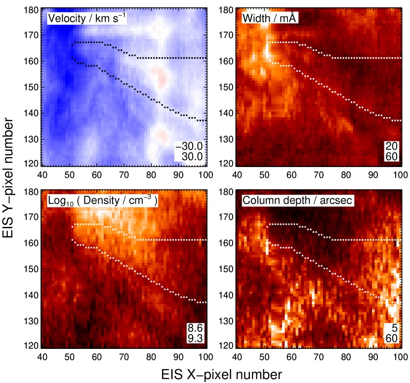
Figure 13: Plasma parameter maps derived from emission lines of Fe xii for the same raster sub-region shown in Fig. 6. The top-left and top-right panels show velocity and line width maps obtained from the $\lambda$195.12 emission line. The bottom-left and bottom-right panels show density and column depth maps derived from the ($\lambda$186.85+$\lambda$186.89)/$\lambda$195.12 ratio. In each plot the loop structure B is indicated by the two dotted lines. The two numbers in the bottom-right corner of each panel give the minimum and maximum value displayed in the images.

The most striking feature of the $\lambda$195.12 velocity map is the blueshifted region to solar-east of the loop footpoints, which also coincides with larger line widths. Comparing also with the $\lambda$195.12 intensity image of Fig. 6 shows that the $\lambda$195.12 intensity is lower in this region. These three features are a signature of so-called active region outflow regions (Del Zanna, 2008; Doschek et al., 2008; Bryans et al., 2010). We note that the $\lambda$195.12 profiles from the present region do not show the distinct emission component on the blue side of the emission line that was found by Bryans et al. (2010) for an active region observed in 2007 December. Instead the line profile is fit well with a single Gaussian. The overlay of the loop B outline on the Fig. 13 images shows that the Fe viii footpoint actually lies within the Fe xii outflow region. Although the blueshifts are strongest at the base of the loop, and just to solar-east of the base, there are significant blueshifts along the body of the loop up to X-pixels of around 70, and also the regions surrounding the loop. This suggests that the outflowing, low intensity plasma may be intermingled with the brighter loops. Note that at X-pixels 80–90 the velocity measurements are consistent with no net line-of-sight flow. We speculate that this region corresponds to loops and, in particular, the features labeled A–D in Fig. 6. Along the body of loop B there is a trend of increasing line width and blueshift towards the footpoint, which may indicate an increasing contribution to the line of sight emission from the outflow region plasma.

The density and column depth maps of Fig. 13 reveal densities of around $\log\,N_{\rm e}$=8.75–9.00 and column depths of 30–60 arcsec for the X-pixel region 80–100. These column depths are consistent with the size of the long loop structures that are seen extending from the footpoint region in the STEREO 195 images of Fig. 7. Towards the base of loop structure B (X-pixels 50–75) the densities are in the range $\log\,N_{\rm e}$=8.95–9.15 and the column depths in the range 12–23″. Sect. 7 suggested that this region (corresponding to the Fe x “brightness patch”) may represent loops that connect to a different spatial location than the loops in the X-pixel region 80–100. However, inspection of the STEREO images of Fig. 7 suggests that both sets of loops have similar heights and brightnesses which should be reflected in similar density and column depths. This is not the case and so there may be low-lying Fe xii emission that is co-spatial with Fe viii and Fe x, although rather more diffuse than these ions.

In summary, the Fe xii emission around the loop footpoints is rather complex. There are large, extended loops with heights of up to 60″ that extend away from the footpoints, probably at multiple angles to the line-of-sight. There is denser, low-lying plasma surrounding the cool footpoints, and there is outflowing plasma neighboring, and probably intermingling, with the loops that is around a factor 2–3 times less intense than the loop emission.

11 Discussion

The most significant result from this work is that a single loop structure observed with EIS exhibits significantly different line-of-sight velocities in two emission lines that are relatively close in temperature. Fe viii $\lambda$185.21 shows a redshift of $\approx 15$ km s^-1  while Fe x $\lambda$184.54 shows velocities close to 0 km s^-1. The differences apply at the same spatial locations in the loop, and are sustained over a projected distance of 9 Mm along the length of the loop. An immediate consequence is that the loop consists of at least two plasma components at different temperatures: one is cool and downflowing, the other is hot and at rest. The fact that the velocity difference is maintained over a large spatial distance means that the two components represent two distinct structures rather than, e.g., the loop simply showing downflows near the bottom, cooler part of the loop and stationary plasma in the upper, hotter part of the loop. The higher spatial resolution of the TRACE instrument revealed that the EIS loop probably consists of at least two narrow ‘strands’ visible at 1 MK in the 171 filter (Fig. 6). However, since both strands are emitting at 1 MK then they will both contribute to the EIS Fe x $\lambda$184.54 emission line and so do not represent the two velocity components.

This result has important consequences if it is treated as a general property of fan loops. Consider, for example, the work of Winebarger et al. (2002) who found Ne viii redshifts in fan loops identified from TRACE 171 images. The authors proceeded to make a loop model with a steady flow that could reproduce the TRACE 171 intensity profile along the loop. Since Ne viii is formed at the same temperature as Fe viii then the redshift result is consistent with the present work (although the magnitude of the velocity was significantly larger in the Winebarger et al., 2002, loop system). The TRACE 171 channel is dominated by Fe x with a smaller contribution from Fe ix. If our EIS result is extrapolated to the Winebarger et al. (2002) loop system, then the TRACE 171 emission has little or no physical relation to the Ne viii emission, and so the Ne viii velocity result can not be included in a model that seeks to interpret the intensity variation in the 171 loop image.

One concept for how the loop may be physically structured is shown in Fig. 14. Two distinct loop types (or strands) are shown. Type 1 is stationary and emits Fe x along a large portion of its length, while type 2 is downflowing and emits Fe viii along a large portion of its length. The “centroid” of the Fe x emission in the type 1 strand is located somewhat higher than that of Fe viii in the type 2 strand, as suggested by the EIS images (Fig. 6). Since the type 1 strand must cool before descending into the photosphere, it must also emit Fe viii emission, but this emission will be much more compact than that coming from the type 2 strand. We note that the velocity of Fe viii $\lambda$185.21 does fall at the lowest heights in the EIS loop (Fig. 9) and the width increases (Fig. 11) which may indicate that the type 1 strand is contributing significant Fe viii emission.

One question relates to the presence of any emission in type 2 strands from ions hotter than Fe viii. It would be surprising if the strand did not achieve coronal temperatures, yet the coronal emission lines observed by EIS show that such emission either does not partake in the Fe viii flow, or that it is sufficiently weak that it is masked by the stationary coronal plasma of the type 1 strands.

Figure 14: A conceptualization of the two types of loop strand that could explain the EIS velocity results. See text for more details.

The work of Del Zanna (2008), Tripathi et al. (2009), Del Zanna (2009a) and Warren et al. (2011) suggests that the velocity results found here may be a common feature of fan loops. If this is correct then, despite the division of the loop into two types of independent strand, these two strands always appear together in fan loops, and their relative distribution/strength always conspires to make Fe x appear stationary and Fe viii downflowing. If there was significant imbalance towards type 1 strands, then Fe viii would no longer display extended emission, instead being compressed into a small spatial region at the base of the Fe x strand. While an imbalance towards type 2 strands would yield a fan loop with either little Fe x emission, or with a Fe x line profile showing significant downflow velocity. A natural solution to the apparent connectedness of the two strand types is that the type 2 strand represents a later, cooling stage in the evolution of a type 1 strand. However, the number of stationary strands is well-balanced with the number of cooling, downflowing strands in order that a predominance of one over the other is not seen in the observations.

These arguments are somewhat speculative and require a survey of many loops before they can be confirmed. Certainly a check on the velocity difference between Fe viii and Fe x needs to be performed on many loops from different active regions. A thorough velocity analysis such as the one presented in this work is not necessary. Simply measuring the wavelength separation of the nearby Fe viii $\lambda$185.21 and Fe x $\lambda$184.54 lines in the loops and comparing with the standard, off-limb rest separation will be sufficient. A study in the same loops of the intensity distributions of the Fe viii and Fe x lines with height would also be profitable by determining the heights of maximum emission. A time history of how the Fe viii–Fe x velocity difference changes (or does not change) for a loop is also an important study, as it may reveal if the balance between type 1 and type 2 strands changes with time.

The concept of apparently monolithic loop structures consisting of multiple, unresolved strands has been explored previously by theorists, particularly with regard the nanoflare theory of coronal heating (Parker, 1988; Cargill, 1994), where small heating events only heat individual strands, but combined can account for global loop properties such as temperature, density and emission measure. Multi-stranded loop models have also been cited to explain observations that appear to show some loops have an isothermal temperature profile (Lenz et al., 1999; Reale & Peres, 2000).

Dynamic, 1D models of individual loops/strands that include plasma flows have been made by Spadaro et al. (2003), Spadaro et al. (2006) and Bradshaw et al. (2010). Spadaro et al. (2003) considered active region loops of 40–80 Mm in length, with peak temperatures of around 4 MK and coronal densities of up to $2\times 10^{10}$ cm^-3; while Spadaro et al. (2006) modeled quiet Sun loops with lengths of 5–10 Mm, peak temperatures up to 1.3 MK, and coronal densities up to $10^{9}$ cm^-3. The parameters of the loop modeled by Bradshaw et al. (2010) are closest to those of the loop studied here – a loop length of 67 Mm, peak temperature of 3.6 MK and density of $3\times 10^{9}$ cm^-3 – so we summarize briefly the velocity results from this work. The loop was allowed to reach a hydrostatic equilibrium with a coronal apex temperature and cool footpoints, and then allowed to cool with no heating applied. Enthalpy and conduction fluxes balance the radiative losses of the plasma, and Bradshaw et al. (2010) found that the enthalpy flux dominates in certain temperature regimes and evolution periods. As the loop progressively cools, increasing downflows are found near the peak temperature of the loop, varying from $\approx$10 km s^-1 around 2 MK to $\approx$40 km s^-1 at 0.3 MK. At the temperatures at which Fe viii and Fe x are formed (0.7–1.1 MK) the velocities are around 15–20 km s^-1, and most of the length of the loop shows significant downflows. The Fe viii velocity measured in “loop structure B” of the present work is consistent with this model, but the flow is only found in the lower portion of the loop, and Fe x shows no significant velocity.

The model can not be directly compared with the observation as the observed loop likely consists of many strands, and so a better comparison would be with a time-average of cooling strands randomly distributed in time. Even then, there is likely a contribution to the emission line intensities and velocities from the heating phase of the strands which is not modeled by Bradshaw et al. (2010). The Fe viii–Fe x velocity result presented here would seem to be a valuable constraint on loop models of this sort, and modelers are encouraged to investigate how it can be reproduced.

Finally, a comment on coronal velocity measurements. The present paper has laid out the difficulties of determining absolute velocities from the EIS instrument. Although EIS is capable of measuring velocities as precise as 0.5 km s^-1 (Mariska et al., 2008), they are only accurate to, at best, 4 km s^-1. Improved accuracy at EUV wavelengths (i.e., below 912 Å) is unlikely for the forseeable future of solar physics due to the lack of absolute wavelength standards. The only solution appears to be observing coronal lines above the Lyman limit where either a calibration lamp can be used, or photospheric/low chromosphere lines with small velocities that serve as wavelength fiducials can be observed. Since the allowed transitions of all coronal ions are found below 700 Å the emission lines must be observed in second, third or even fourth spectral order, but then blending can become a significant issue. There are some coronal forbidden lines that are found above the Lyman limit but below where the photospheric continuum begins to become significant ($\approx 1400$ Å). The most notable such line is probably Fe xii $\lambda$1242.

12 Summary

A loop footpoint region aligned towards the observer’s line-of-sight has been identified in ions formed from $\log\,T=5.2$ to 6.0, showing a clear progression of hotter emission with greater heights. The continuation of the loop to higher temperatures of $\log\,T=6.1$ to 6.3 is less distinct and suggests two groups of loops that may return to the solar surface at different locations on the opposite side of the active region. Line-of-sight velocities in one particular footpoint show redshifts of around 15–20 km s^-1 for the ions O vi, Mg vi and Fe viii (formed over $\log\,T=5.5$–5.8). A clear and distinct drop to approximately zero velocity is found for Fe x ($\log\,T=6.0$), with the difference in velocity occurring at the same spatial locations and being maintained over a projected spatial region of at least 9000 km. Fe xi and Fe xii, formed at $\log\,T=6.1$–6.2, show velocities consistent with Fe x although the loop structure is probably contaminated by distinct, outflowing plasma along the line-of-sight at low heights.

By comparing the line widths of Fe viii and Fe x it is shown that the different velocities of the two ions imply that the Fe x emission comes from a different structure (or structures) than Fe viii despite the fact that the loops visible in the ions’ images are co-spatial. The solution suggested here is that there are two distinct types of strand within the loop: one is hot and stationary, the other is cooler and downflowing. The second strand may simply represent a later stage of evolution of the first strand, but in this case there must be many strands that average out to give the observed loop emission.

A density diagnostic of Mg vii was used to demonstrate that the density falls monotonically with height from $\log\,N_{\rm e}$=9.5 at the base to $\log\,N_{\rm e}$=8.6 at a projected height of 15,000 km. Assuming a circular cross-section for the loop structure, the filling factor is estimated to increase from around 0.05 at the loop base to close to 0.3 at 15,000 km. Over the region where there is a difference in line-of-sight velocity for Fe viii and Fe x the filling factor is around 0.2. As Mg vii is formed at a similar temperature to Fe viii, this filling factor result supports the conclusion that the Fe viii emission comes from only a fraction of the loop volume, with the Fe x emitting strands contributing to some part of the remaining volume.

Inspection of line parameter maps from Fe xii shows that the loop structure considered here lies very close to, or even within, an active region outflow region. These regions appear to be common to many active regions, and their close proximity to fan loops has previously been noted by Warren et al. (2011). Mixing of the outflow plasma along of the line-of-sight to the loop structure complicates velocity measurements for Fe xi and Fe xii.

Appendix A Comparison between the quiet Sun and HK methods for wavelength calibration

The empirical model of Kamio et al. (2010) allows the absolute wavelength of the Fe xii $\lambda$195.12 emission line at an instance in time to be determined purely from instrument temperature measurements and the motion of the Hinode spacecraft. We can use this method to determine the average velocity of Fe viii $\lambda$185.21 in the quiet Sun part of the 2009 November 21 raster and compare it to the method described in Sect. 6.1. The data are processed in the same way, and so the bottom 50 pixels of the $\lambda$185.21 raster are averaged to produce a spectrum with good signal-to-noise. Instead of the orbit variation being determined from the variation of the $\lambda$185.21 centroid, however, it is taken from the Kamio et al. (2010) method. Since this method corrects the EIS wavelength scale to force $\lambda$195.12 to be at rest, then it is necessary to apply the off-limb offset of Warren et al. (2011) to obtain the rest wavelength of $\lambda$185.21. Upon doing this, the velocity in the quiet Sun region can be obtained and the results are shown in Fig. 15. The $\lambda$185.21 velocities are mostly redshifts, and the average quiet Sun velocity over the complete X-pixel range is $+2.8$ km s^-1, compared to the value of $-2.6$ km s^-1 that was used in Sect. 6.1, so there is a systematic offset of 5.4 km s^-1 between the two calibration methods. The quiet Sun calibration method used in the present work is preferred as it is tied to the absolute quiet Sun velocity measurements of Peter & Judge (1999), whereas the method of Kamio et al. (2010) makes the assumption that the Fe xii $\lambda$195.12 velocity measured over the life of the EIS mission averages to zero, which may not be true.

Figure 15: Absolute Fe viii $\lambda$185.21 velocites in the quiet Sun part of the 2009 November 11 raster obtained using the method of Kamio et al. (2010). The dashed horizontal line denotes the quiet Sun velocity assumed for the calibration method described in Sect. 6.1. The X-pixel range that corresponds to the coronal loop is indicated.

References

- Bradshaw et al. (2010) Bradshaw, S. J. & Cargill, P. J. 2010, ApJ, 710, L39
- Brekke et al. (1997) Brekke, P., Hassler, D. M., & Wilhelm, K. 1997, Sol. Phys., 175, 349
- Brooks et al. (2009) Brooks, D. H., Warren, H. P., Williams, D. R., & Watanabe, T. 2009, ApJ, 705, 1522
- Brooks et al. (2011) Brooks, D. H., Warren, H. P., & Young, P. R. 2011, ApJ, 730, 85
- Brown et al. (2008) Brown, C. M., Feldman, U., Seely, J. F., Korendyke, C. M., & Hara, H. 2008, ApJS, 176, 511
- Bryans et al. (2010) Bryans, P., Young, P. R. & Doschek, G. A., 2010, ApJ, 715, 1012
- Cargill (1994) Cargill, P. J. 1994, ApJ, 422, 381
- Cheng et al. (1980) Cheng, C.-C., Smith, J. B., Jr., Tandberg-Hanssen, E. 1980, Sol. Phys., 67, 259
- Culhane et al. (2007) Culhane, J. L., Harra, L. K., James, A. M., et al. 2007, Solar Physics, 243, 19
- Delaboudinière et al. (1995) Delaboudinière, J.-P., Artzner, G. E., Brunaud, J., et al. 1995, Sol. Phys., 162, 291
- Del Zanna (2008) Del Zanna, G. 2008, A&A 481, L49
- Del Zanna (2009a) Del Zanna, G. 2009a, A&A, 508, 501
- Del Zanna (2009b) Del Zanna, G. 2009b, A&A, 508, 513
- De Moortel et al. (2002) De Moortel, I., Ireland, J., Walsh, R. W., & Hood, A. W. 2002, Sol. Phys., 209, 61
- De Pontieu & McIntosh (2010) De Pontieu, B. & McIntosh, S. W. 2010, ApJ, 722, 1013
- Dere et al. (1997) Dere, K. P., Landi, E., Mason, H. E., Monsignori-Fossi, B. C., & Young, P. R. 1997, A&AS, 125, 149
- Dere et al. (2001) Dere K. P., Landi E., Young P. R., & Del Zanna G. 2001, ApJS, 134, 331
- Dere et al. (2009) Dere K. P., Landi E., Young P. R., et al. 2009, A&A, 498, 915
- Domingo et al. (1995) Domingo, V., Fleck, B. & Poland, A. I. 1995, Sol. Phys., 162, 1
- Doschek (2006) Doschek, G. A. 2006, ApJ, 649, 515
- Doschek et al. (2008) Doschek, G. A., Warren, H. P., Mariska, J. T., et al., 2008, ApJ 686, 1362
- Doschek et al. (2007) Doschek, G. A., Mariska, J. T., Warren, H. P., et al. 2007, ApJ, 667, L109
- Feldman & Laming (2000) Feldman, U., & Laming, J. M. 2000, Phys. Scripta, 61, 222
- Foukal (1976) Foukal, P. V. 1976, ApJ, 210, 575
- Handy et al. (1999) Handy, B. N., Action, L. W., Kankelborg, C. C., et al. 1999, Sol. Phys., 187, 229
- Haugan (1999) Haugan, S. V. H. 1999, Sol. Phys., 185, 275
- Feldman et al. (1992) Feldman, U., Mandelbaum, P., Seely, J. L., Doschek, G. A., & Gursky H. 1992, ApJS, 81, 387
- Harra et al. (2008) Harra, L. K., Sakao, T., Mandrini, C. H., et al. 2008, ApJ, 676, L147
- Harrison et al. (1995) Harrison, R. A., Sawyer, E. C., Carter, M. K., et al. 1995, Sol. Phys., 162, 233
- Hassler et al. (1991) Hassler, D. M., Rottman, G. J., & Orrall, F. Q. 1991, ApJ, 372, 710
- Kamio et al. (2010) Kamio, S., Hara, H., Watanabe, T., Fredvik, T. & Hansteen, V. H., 2010, Sol. Phys., 266, 209
- Korendyke et al. (2006) Korendyke, C. M., Brown, C. M., Thomas, R. J., et al. 2006, Appl. Optics, 45, 8674
- Kosugi et al. (2007) Kosugi, T., Matsuzaki, K., Sakao, T. et al. 2007, Sol. Phys., 243, 3
- Lenz et al. (1999) Lenz, D. D., Deluca, E. E., Golub, L., Rosner, R., & Bookbinder, J. A. 1999, ApJ, 517, L155
- Mariska et al. (2007) Mariska, J. T., Warren, H. P., Ugarte-Urra, I., et al. 2007, PASJ, 59, 713
- Mariska et al. (2008) Mariska, J. T., Warren, H. P., Williams, D. R., & Watanabe, T. 2008, ApJ, 681, L41
- Marsch et al. (2004) Marsch, E., Wiegelmann, T., & Xia, L. D. 2004, A&A, 428, 629
- McEwan & De Moortel (2006) McEwan, M. P., & De Moortel, I. 2006, A&A, 448, 763
- Parker (1988) Parker, E. N. 1988, ApJ, 330, 474
- Peter & Judge (1999) Peter, H., & Judge, P. G. 1999, ApJ, 522, 1148
- Reale & Peres (2000) Reale, F., & Peres, G. 2000, ApJ, 528, L45
- Samain (1991) Samain, D. 1991, A&A, 244, 217
- Schrijver et al. (1999) Schrijver, C. J., Title, A. M., Berger, T. E., et al. 1999, Sol. Phys., 187, 261
- Spadaro et al. (2003) Spadaro, D., Lanza, A., Lanzafame, A. C., et al. 2006, ApJ, 582, 486
- Spadaro et al. (2006) Spadaro, D., Lanza, A., Karpen, J. T., & Antiochos, S. K. 2006, ApJ, 642, 579
- Tian et al. (2010) Tian, H., Tu, C., Marsch, E., He, J. & Kamio, S. 2010, ApJ, 709, L88
- Tripathi et al. (2009) Tripathi, D., Mason, H. E., Dwivedi, B. N., Del Zanna, G., & Young, P. R. 2009, ApJ, 694, 1256
- Tripathi et al. (2010) Tripathi, D., Mason, H. E., Del Zanna, G., & Young, P. R. 2010, A&A, 518, A42
- Ugarte-Urra & Warren (2011) Ugarte-Urra, I., & Warren, H. P. 2011, ApJ, 730, 37
- Vernazza & Reeves (1978) Vernazza, J. E., & Reeves, E. M. 1978, ApJS, 37, 485
- Wang et al. (2009) Wang, T. J., Ofman, L., & Davila, J. M. 2009, ApJ, 696, 1448
- Warren et al. (2011) Warren, H. P., Ugarte-Urra, I., Young, P. R. & Stenborg, G., 2011, ApJ, 727, 58
- Widing & Feldman (2001) Widing, K. G., & Feldman, U. 2001, ApJ, 555, 426
- Wilhelm et al. (1995) Wilhelm, K., Curdt, W., Marsch, E., et al. 1995, Sol. Phys, 162, 189
- Winebarger et al. (2002) Winebarger, A. R., Warren, H. P., van Ballegooijen, A., DeLuca, E. E., & Golub, L. 2002, ApJ, 567, 89
- Young (2009) Young, P. R. 2009, ApJ, 691, L77
- Young (2010) Young, P. R. 2010, EIS Software Note No. 13, ‘Interpolating missing pixels in EIS data’, Version 4 (available at: ftp://sohoftp.nascom.nasa.gov/solarsoft/hinode/eis/doc/eis_notes/13_INTERPOLATION/eis_swnote_13.pdf).
- Young (2011a) Young, P. R. 2011a, EIS Software Note No. 1, ‘EIS_PREP’, Version 3.1 (available at: ftp://sohoftp.nascom.nasa.gov/solarsoft/hinode/eis/doc/eis_notes/1_EIS_PREP/eis_swnote_01.pdf).
- Young (2011b) Young, P. R. 2011b, EIS Software Note No. 16, ‘EIS_AUTO_FIT and SPEC_GAUSS_EIS: Gaussian fitting routines for the Hinode/EIS mission’, Version 2.1 (available at: ftp://sohoftp.nascom.nasa.gov/solarsoft/hinode/eis/doc/eis_notes/16_AUTO_FIT/eis_swnote_16.pdf).
- Young (2011c) Young, P. R. 2011c, EIS Software Note No. 15, ‘Deriving densities, column depths and filling factors from Hinode/EIS data’, Version 2.1 (available at: ftp://sohoftp.nascom.nasa.gov/solarsoft/hinode/eis/doc/eis_notes/15_DENSITY/eis_swnote_15.pdf).
- Young (2011d) Young, P. R. 2011d, EIS Software Note No. 7, ‘Instrumental line widths for the narrow slits of EIS’, Version 0.1 (available at: ftp://sohoftp.nascom.nasa.gov/solarsoft/hinode/eis/doc/eis_notes/07_LINE_WIDTH/eis_swnote_07.pdf).
- Young & Landi (2009) Young, P. R., & Landi, E. 2009, ApJ, 707, 173
- Young & Mason (1997) Young, P. R., & Mason, H. E. 1997, Sol. Phys., 175, 523
- Young et al. (2007a) Young, P. R., Del Zanna, G., Mason, H. E., et al. 2007a, PASJ, 59, S727
- Young et al. (2007b) Young, P. R., Del Zanna, G., Mason, H. E., et al. 2007b, PASJ, 59, S857
- Young et al. (2009) Young, P. R., Watanabe, T., Hara, H., & Mariska, J. T. 2009, A&A, 495, 587