Current fluctuations at a phase transition

Abstract

The ABC model is a simple diffusive one-dimensional non-equilibrium system which exhibits a phase transition. Here we show that the cumulants of the currents of particles through the system become singular near the phase transition. At the transition, they exhibit an anomalous dependence on the system size (an anomalous Fourier’s law). An effective theory for the dynamics of the single mode which becomes unstable at the transition allows one to predict this anomalous scaling.

A lot of work has been devoted recently to the study of the fluctuations of the current of heat or of particles through non-equilibrium one dimensional systems BD ; BDGJL5 ; BBO ; derrida2007 ; HS2 ; ADLW ; ILW ; HG ; HG2 ; PM2 ; Tou ; LM2 . In such studies the basic quantity one considers is the total flux $Q(t)$ of energy or of particles through a section of the system during time $t$. In the steady state this flux $Q(t)$ fluctuates due to the randomness of the initial condition for purely deterministic models and due to the noisy dynamics in stochastic models (here we only discuss classical systems: see LLY ; Be ; BB ; RB for the quantum case). If one assumes that the total energy or the total number of particles in the system remains bounded, the average current $\lim_{t\to\infty}{\langle Q(t)\rangle\over t}$ as well as the higher cumulants $\lim_{t\to\infty}{\langle Q(t)^{n}\rangle_{c}\over t}$ of the flux $Q(t)$ do not depend on the section of the system where this flux is measured.

For a one dimensional system of length $L$, a central question is the size dependence of these cumulantsBLR . In particular one would like to know whether a given system satisfies Fourier’s law, meaning that, for large $L$, the average current scales like $1/L$:

$$\lim_{t\to\infty}{\langle Q(t)\rangle\over t}\simeq{A_{1}\over L}$$ (1)

where the prefactor $A_{1}$ depends on the temperatures $T_{1}$ and $T_{2}$ of the two heat baths or on the chemical potentials $\mu_{1}$ and $\mu_{2}$ of the two reservoirs of particles at the ends of the system. At equilibrium ($T_{1}=T_{2}$ or $\mu_{1}=\mu_{2}$) the prefactor $A_{1}$ in (1) vanishes but the question of the validity of Fourier’s law remains. One then wants to know whether the second cumulant of $Q(t)$ scales like $1/L$.

$$\lim_{t\to\infty}{\langle Q(t)^{2}\rangle-\langle Q(t)\rangle^{2}\over t}=\lim_{t\to\infty}{\langle Q(t)^{2}\rangle_{c}\over t}\simeq{A_{2}\over L}\,.$$ (2)

One can show that (2) holds for diffusive systems such as the SSEP (symmetric simple exclusion process)BD ; derrida2007 ; DDR ; HS or the KMP (Kipnis-Marchioro-Presutti) modelKMP . The macroscopic fluctuation theory developed by Bertini et al. BDGJL5 ; BDGJL6 ; BDGJL3 allows one also to determineBD all the cumulants of the flux $Q(t)$, with the result that they all scale with system size as $1/L$.

$$\lim_{t\to\infty}{\langle Q(t)^{n}\rangle_{c}\over t}\simeq{A_{n}\over L}$$ (3)

Even corrections of order $1/L^{2}$ have been computed in some casesADLW ; ILW .

For mechanical systems with deterministic dynamics, in particular systems which conserve momentum, the average current scales as a non-integer power of the system size:

$$\lim_{t\to\infty}{\langle Q(t)\rangle\over t}\simeq{B_{1}\over L^{1-\alpha}}$$

The exponent $\alpha$ takes the value $1/2$ for some exactly soluble special modelsBBO . Values ranging from 0.25 to 0.4 have also been reported in simulations depending on the model consideredLW ; MDN ; GNY ; Dhar2 ; GDL . Theoretical predictions based on a mode coupling approachLLP ; LLP2 or on renormalization group calculationsDhar confirm this anomalous Fourier’s law. Less is known on the size dependence of the higher cumulants, which are numerically harder to measure, except that they vary as power laws of the system size, with exponents which seem to depend on the geometryBDG .

Here we consider the $ABC$ modelEKKM ; EKKM2 , a diffusive system which is known to exhibit a phase transitionCDE ; ACLMMS ; LM ; BLS ; LCM : we study the fluctuations of the current near this transition. Generically, outside the transition the cumulants have a diffusive scaling (3). Here, we show that the amplitudes $A_{n}$ become singular as one approaches the transition, and that the cumulants of $Q(t)$ exhibit anomalous scalings at the transition. When the transition is second order, due to the destabilization of a single Fourier mode of the densityCDE , the fluctuations in the whole critical regime can be understood in terms of a Langevin equation for a single complex variable which represents the amplitude and the phase of this Fourier mode.

I Definition

The $ABC$ modelEKKM ; EKKM2 ; CDE ; ACLMMS ; LM ; BLS ; LCM is a one-dimensional lattice gas, where each site is occupied by one of three types of particles, $A$, $B$ and $C$. Neighboring sites exchange particles at the rates

$$AB \underset{1}{\overset{q}{\rightleftharpoons}}BA$$

$$BC \underset{1}{\overset{q}{\rightleftharpoons}}CB$$

$$CA \underset{1}{\overset{q}{\rightleftharpoons}}AC$$

with an asymmetry $q\leq 1$. Here, we consider the model on a ring of $L$ sites. Since the rates are invariant under cyclic permutations of $\{A,B,C\}$ , most of the equations below will be written for a species $a\in\{A,B,C\}$, with $b$ and $c$ denoting respectively the next and previous species. When $q$ scales as

$$q=e^{-\beta/L}\,,$$

the dynamics become diffusive: in particular, the probability that site $1\leq k\leq L$ is occupied by a particle of type $a$ behaves as

$${\rm Pro}[s_{k}(t)=a]\simeq\rho_{a}(k/L,t/L^{2})\,,$$

where the macroscopic density profiles $\rho_{a}(x,\tau)$ follow a local Fourier’s law : if $j_{a}(x,\tau)$ is the current associated to $\rho_{a}$, then

$$j_{a}=-\partial_{x}\rho_{a}+\beta\rho_{a}(\rho_{c}-\rho_{b})\,,$$ (4)

which, together with the conservation law

$$\partial_{\tau}\rho_{a}=-\partial_{x}j_{a}\,,$$ (5)

gives the hydrodynamic equationsCDE satisfied by the density:

$$\partial_{\tau}\rho_{a}=\partial_{x}^{2}\rho_{a}+\beta\partial_{x}\rho_{a}(\rho_{b}-\rho_{c})\,.$$ (6)

These equations conserve the fact that $\sum_{a}\rho_{a}(x,\tau)=1$ (each site is occupied by one of the three species) and $\int_{0}^{1}dx\rho_{a}(x,\tau)=r_{a}$, where $r_{a}$ is the total density of particles of type $a$. The deterministic equations (4) and (6) are only valid in the large $L$ limit, for diffusive time scales, i.e. $t\sim L^{2}$.

For small $\beta$, the constant density profiles $\rho_{a}(x)=r_{a}$ are a stable stationnary solution of (6). These constant profiles become linearly unstable above a critical value $\beta_{*}$CDE given by

$$\beta_{*}={2\pi\over\sqrt{\Delta}}\;\;\mbox{ with }\;\;\Delta=1-2\sum_{a}r_{a}^{2}\,,$$ (7)

so that the long-time limit of (6) becomes a function $\bar{\rho}_{a}(x)$ of the space variable $x$ for $\beta>\beta_{*}$. It has been arguedBD2 (and checked numerically) that, in the steady state, these modulated profiles do not move. If the phase transition to the modulated phase is second order, then it should occur at $\beta=\beta_{*}$ given by (7). A first-order transition may however occur at $\beta<\beta_{*}$ : this should certainlyCDE be the case at least for $\Lambda<0$, with

$$\Lambda=\sum r_{a}^{2}-2\sum r_{a}^{3}\,.$$ (8)

In the following, we study the integrated current $Q_{A}(t)$ of $A$ particles through the system during time $t$:

$$Q_{A}(t) ={1\over L}\int_{0}^{t}dt^{\prime}\int_{0}^{1}dx\;j_{A}(x,t^{\prime})dt^{\prime}$$

$$=L\int_{0}^{t/L^{2}}d\tau\int_{0}^{1}dx\;j_{A}(x,\tau)d\tau\,.$$ (9)

This space average fluctuates with time, and we will be interested in its cumulants, as in (3). Because the difference between the space average and the flux through a section remains bounded, the cumulants of the flux through any section are the same as those of this space average in the long time limitBD2 .

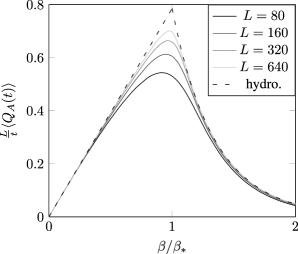
Figure 1: First cumulant of the integrated current of $A$ particles in the $ABC$ model with $r_{A}=r_{B}=1/4$, for $0\leq\beta\leq 2\beta_{*}$. Measurements of $\langle Q_{A}\rangle$ in Monte-Carlo simulations of systems of $80$ to $640$ sites are compared to the prediction of the hydrodynamic equation (11).

II Mean current

As the steady-state profiles $\bar{\rho}_{a}(x)$ are time independentBD2 , (5) implies that the steady-state currents are constant, $\bar{j}_{a}(x)=J_{a}$. They are given by

$$J_{a}=\beta\int_{0}^{1}dx\bar{\rho}_{a}(x)(\bar{\rho}_{c}(x)-\bar{\rho}_{b}(x))\,.$$ (10)

Then, from (I),

$${\langle Q_{A}(t)\rangle\over t}\sim{{\beta}\over L}\int dx\bar{\rho}_{A}(x)(\bar{\rho}_{C}(x))-\bar{\rho}_{B}(x))\,.$$ (11)

$\langle Q_{A}(t)\rangle$ can thus be obtained by calculating numerically the long-time limit of (6) and then integrating (10). In Figure 1, we compare the results of this calculation to numerical measurements obtained by simulating finite systems of $80$ to $640$ sites, for $r_{A}=r_{B}=1/4$ and $0\leq\beta\leq 2\beta_{*}$, with $\beta_{*}$ given by (7).

For $\beta\leq\beta_{*}$, the stability of the flat density profiles $\bar{\rho}_{a}(x)=r_{a}$ leads to a current $\langle Q_{A}(t)\rangle\sim{t\over L}\beta r_{A}(r_{C}-r_{B})$; on the other hand, the dependence in $\beta$ becomes non-trivial for $\beta>\beta_{*}$, with a cusp at $\beta_{*}$.

For $\beta\downarrow\beta_{*}$, the steady-state profiles are known (see CDE or (27) and (28) below) to take the form

$$\bar{\rho}_{a}(x)=r_{a}+\sqrt{\beta-\beta_{*}}(K_{a}e^{2i\pi x}+cc.)+{\mathcal{O}}(\beta-\beta_{*})$$ (12)

with known constants $K_{A}$, $K_{B}$ and $K_{C}$, leading to an analytic expression for $\langle Q_{A}(t)\rangle$ around $\beta_{*}^{+}$:

$${L\over t}\langle Q_{A}(t)\rangle\underset{\beta\downarrow\beta_{*}}{\simeq}(r_{C}-r_{B})\left[\beta r_{A}-{\Delta^{2}\over\Lambda}(\beta-\beta_{*})\right]\,.$$

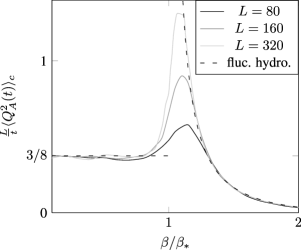
Figure 2: Second cumulant of the integrated current of $A$ particles in the $ABC$ model with $r_{A}=r_{B}=1/4$, for $0\leq\beta\leq 2\beta_{*}$. Measurements of $\langle Q_{A}^{2}\rangle_{c}$ in systems with $80$ to $320$ sites are compared to those obtained from the macroscopic fluctuation theory (13,14).

III Fluctuation theory

The hydrodynamic equations (6) describe the deterministic evolution of the density profiles $\rho_{a}(x,\tau)$ in the large $L$ limit. For a large, but finite system, one has to take into account stochastic corrections. This can be done using fluctuating hydrodynamics, where the expression (4) of the current is replaced withderrida2007 ; HS

$$j_{a}=q_{a}+{1\over\sqrt{L}}\eta_{a}(x,\tau)$$ (13)

where $q_{a}=-\partial_{x}\rho_{a}+\beta\rho_{a}(\rho_{c}-\rho_{b})$ is the right-hand side of (4), and where the $\eta_{a}$ are Gaussian noises such that $\sum_{a}\eta_{a}=0$ and

$$\langle\eta_{a}(x,\tau)\eta_{a^{\prime}}(x^{\prime},\tau^{\prime})\rangle=\sigma_{aa^{\prime}}(x,\tau)\delta(x-x^{\prime})\delta(\tau-\tau^{\prime})\,,$$

with $\sigma_{aa}=2\rho_{a}(1-\rho_{a})$ and $\sigma_{aa^{\prime}}=-2\rho_{a}\rho_{a^{\prime}}$ for $a\neq a^{\prime}$. Alternatively, the macroscopic fluctuation theoryBDGJLX expresses (13) as a large deviation principle, with the probability of observing time-dependent density profiles $\rho_{a}(x,\tau)$ given by

$${\rm Pro}[\rho_{a}(x,\tau)]\propto\exp\left[-L\iint dxd\tau\sum_{a}{(j_{a}-q_{a})^{2}\over 4\rho_{a}}\right]\;.$$

From this formulation, the generating function of the current $Q_{A}(t)$ is the solution of the optimization problem

$$\log\langle e^{\lambda Q_{A}(t)}\rangle=\max_{\rho_{a},j_{a}}L\int_{0}^{t/L^{2}}d\tau\int dx\left[\lambda j_{A}-\sum_{a}{(j_{a}-q_{a})^{2}\over 4\rho_{a}}\right]\,.$$ (14)

Finding the density and current profiles $\rho_{a}(x,\tau)$ and $j_{a}(x,\tau)$ which maximize (14) is not an easy task. We assume that, for large $t$, the optimum in (14) is achieved by profiles of fixed shape which may drift with a constant velocity $v$. In order to obtain $\langle Q_{A}^{2}(t)\rangle_{c}$, we compute $\log\langle e^{\lambda Q_{A}(t)}\rangle$ to order $2$ in $(\lambda,v)$, before optimizing over $v$: one then gets optimization equations satisfied by these moving profiles, which we solved numerically in the case $r_{A}=r_{B}=1/4$ for $0\leq\beta\leq 2\beta_{*}$.

For $\beta<\beta_{*}$, the constant profiles $\bar{\rho}_{a}(x)=r_{a}$ are still optimal for $\lambda\neq 0$, yielding

$$\langle Q_{A}^{2}(t)\rangle_{c}\simeq{2t\over L}r_{A}(1-r_{A})\,.$$

For $\beta>\beta_{*}$, one has to take into account the dependence of the optimal profiles in $v$ and $\lambda$. This leads (as will be shown in the longer DG2 ) to a second cumulant which diverges at $\beta=\beta_{*}$. This divergence can be computed exactly thanks to the knownledge of the steady-state profiles (12) for $\beta\downarrow\beta_{*}$, leading to

$$\langle Q_{A}^{2}(t)\rangle_{c}\underset{\beta\downarrow\beta_{*}}{\simeq}{t\over L}{12\pi r_{A}r_{B}r_{C}(r_{B}-r_{C})^{2}\over\Lambda\sqrt{\Delta}(\beta-\beta_{*})}\,.$$

IV Critical regime for the deterministic hydrodynamics

In this section, we analyse how the deterministic equations (6), exact in the $L\to\infty$ limit, behave in the neighborhood of $\beta_{*}$. The stability analysis of the constant profiles $\rho_{a}=r_{a}$ shows that, as $\beta$ crosses $\beta_{*}$, only the first Fourier modes of the $\rho_{a}$ become unstable. For $\beta$ close to $\beta_{*}$, one therefore expects this mode to relax more slowly than the other Fourier modes.

One can write, from (6), an evolution equation for these slow modes when $\beta$ is close to $\beta_{*}$, and show that they decay as a power law (instead of an exponential) in the critical regime. To do so, we separate in $\rho_{a}(x,\tau)$ the first Fourier mode, $R_{a}(\tau)e^{2i\pi x}$, from the other modes, $\tilde{\rho}_{a}(x,\tau)$, so that

$$\rho_{a}(x,\tau) =r_{a}+R_{a}(\tau)e^{2i\pi x}+cc.+\tilde{\rho}_{a}(x,\tau)\,,$$ (15)

$$j_{a}(x,\tau) =J_{a}(\tau)+{i\over 2\pi}\dot{R}_{a}e^{2i\pi x}+cc.-\partial_{\tau}\int_{0}^{x}dy\tilde{\rho}_{a}(y,\tau)$$

with $\tilde{\rho}_{a}\ll R_{a}\ll r_{a}$. We also suppose that $\rho_{a}(x,\tau)$ varies slowly, so that $\partial_{\tau}R_{a}\equiv\dot{R}_{a}\ll R_{a}$ and $\partial_{\tau}\tilde{\rho}_{a}\ll\tilde{\rho}_{a}$; finally, we set

$$\beta=\beta_{*}(1+\gamma)$$

with $\gamma\ll 1$. The leading order of (4) then becomes, when projected on the first and second Fourier modes,

$$2i\pi R_{a}= \beta_{*}[R_{a}(r_{c}-r_{b})+r_{a}(R_{c}-R_{b})]$$ (16)

$$\partial_{x}\tilde{\rho}_{a}= \beta_{*}[\tilde{\rho}_{a}(r_{c}-r_{b})+r_{a}(\tilde{\rho}_{c}-\tilde{\rho}_{b})$$

$$+R_{a}(R_{c}-R_{b})e^{4i\pi x}+cc.]$$ (17)

Equation (16) relates the leading orders of $R_{B}$ and $R_{C}$ to $R_{A}$, so that

$$\left\{\begin{array}[]{l}R_{B}(\tau)={2r_{C}-1-i\sqrt{\Delta}\over 2r_{A}}R_{A}(\tau)+x_{B}(\tau)\\ R_{C}(\tau)={2r_{B}-1+i\sqrt{\Delta}\over 2r_{A}}R_{A}(\tau)+x_{C}(\tau)\end{array}\right.$$ (18)

with $x_{B},x_{C}\ll R_{A}$. Equation (17) shows that, at leading order, $\tilde{\rho}_{a}$ is of the form

$$\tilde{\rho}_{a}(x,\tau)=\varphi_{a}e^{4i\pi x}+cc.$$ (19)

with

$$4i\pi\varphi_{a}=\beta_{*}[\varphi_{a}(r_{c}-r_{b})+r_{a}(\varphi_{c}-\varphi_{b})+R_{a}(R_{c}-R_{b})]\,,$$

whose solution is

$$\varphi_{a}={1-2r_{a}\over\Delta}R_{a}^{2}\,.$$ (20)

Then, the next-to-leading order of the first Fourier mode of (4) reads

$${i\over 2\pi}\dot{R}_{a}= 2i\pi\gamma R_{a}+\beta_{*}[(r_{c}-r_{b}-i\sqrt{\Delta})x_{a}+r_{a}(x_{c}-x_{b})$$

$$+\varphi_{a}(R^{*}_{c}-R^{*}_{b})+R_{a}^{*}(\varphi_{c}-\varphi_{b})]$$ (21)

(with $x_{A}\equiv 0$). The $x_{a}$ can be eliminated by multiplying the equation over $\dot{R}_{A}$ by $(r_{C}-r_{B}+i\sqrt{\Delta})$, the one over $\dot{R}_{C}$ by $r_{A}$, the one over $\dot{R}_{B}$ by $-r_{A}$, and by summing, which yields

$$\dot{R}_{A}=4\pi^{2}\left(\gamma-{2\Lambda\over\Delta^{2}}{|R_{A}|^{2}\over r_{A}}\right)R_{A}\,,$$ (22)

with $\Lambda$ given by (8).

For $\beta=\beta_{*}$ ($\gamma=0$), the first Fourier mode $R_{A}$ decays as a power law instead of an exponential:

$$R_{A}(\tau)={R_{A}(0)\over\sqrt{1+{16\pi^{2}\Lambda\over r_{A}\Delta^{2}}|R_{A}(0)|^{2}\tau}}\,,$$

with an amplitude which does not depend on the initial condition for large $\tau$.

V Critical behavior of the MFT

We now return to the noisy equation (13) and try to obtain a noisy version of (22). By analogy with the deterministic case above, we suppose that the first Fourier mode $R_{a}$ of $\rho_{a}$ varies more slowly, but with a larger amplitude than the other modes, so that $\dot{R}_{a}\ll R_{a}$ and $\tilde{\rho}_{a}\ll R_{a}$ in (15). When replacing (4) with (13) ,the leading-order equation (16) is not modified, so that (18) still holds : however, the next-to-leading order equation (21) is replaced with

$${i\over 2\pi}\dot{R}_{a}= 2i\pi\gamma R_{a}+\beta_{*}[(r_{c}-r_{b}-i\sqrt{\Delta})x_{a}+r_{a}(x_{c}-x_{b})$$

$$+\varphi_{a}(R^{*}_{c}-R^{*}_{b})+R_{a}^{*}(\varphi_{c}-\varphi_{b})]+{\nu_{a}(\tau)\over\sqrt{L}}\,,$$ (23)

where the $\nu_{a}$ are projections of the $\eta_{a}(x,\tau)$ on the first Fourier mode:

$$\nu_{a}(\tau)=\int_{0}^{1}dxe^{-2i\pi x}\eta_{a}(x,\tau)\,,$$

so that $\langle\nu_{a}(\tau)\nu^{*}_{a^{\prime}}(\tau^{\prime})\rangle=\sigma_{aa^{\prime}}\delta(\tau-\tau^{\prime})$ and $\langle\nu_{a}(\tau)\nu_{a^{\prime}}(\tau^{\prime})\rangle=0$. The second Fourier modes $\varphi_{a}$ (19) satisfy the equations

$${i\over 4\pi}\dot{\varphi}_{a}= -4i\pi\varphi_{a}+\beta_{*}[\varphi_{a}(r_{c}-r_{b})+r_{a}(\varphi_{c}-\varphi_{b})$$

$$+R_{a}(R_{c}-R_{b})]+{\nu_{a}^{(2)}(\tau)\over\sqrt{L}}\,,$$

where the $\nu_{a}^{(2)}$ are projections of the $\eta_{a}(x,\tau)$ as well : hence, they fluctuate around their non-noisy expression (20). In (23), however, these fluctuations (of amplitude $1/\sqrt{L}$) are multiplied by $R_{a}^{*}$, so that they are of smaller amplitude than the noisy term $\nu_{a}(\tau)/\sqrt{L}$ : therefore, the $\varphi_{a}$ can be replaced by their expression (20) in (23).

Taking a linear combination of (23) to eliminate the $x_{a}$ as in the deterministic case (21), we then obtain

$$\dot{R}_{A}=4\pi^{2}\left(\gamma-{2\Lambda\over\Delta^{2}}{|R_{A}|^{2}\over r_{A}}\right)R_{A}+{\mu_{A}(\tau)\over\sqrt{L}}\,,$$

with $\mu_{A}$ a linear combination of the $\nu_{a}$, which verifies

$$\langle\mu_{A}(\tau)\mu_{A}^{*}(\tau^{\prime})\rangle={24\pi^{2}r_{A}^{2}r_{B}r_{C}\over\Delta}\delta(\tau-\tau^{\prime})\,.$$

Finally, the change of variables

$$R_{A}(\tau)=\sqrt[4]{3\Delta r_{A}^{3}r_{B}r_{C}\over\Lambda L}f(\bar{\tau})\\ \mbox{ with }\bar{\tau}=8\pi^{2}{\sqrt{3\Lambda r_{A}r_{B}r_{C}}\over\Delta^{3/2}}{\tau\over\sqrt{L}}$$ (24)

leads to a simple rescaled equation:

$${df\over d\bar{\tau}}=(\bar{\gamma}-|f(\bar{\tau})|^{2})f(\bar{\tau})+\mu(\bar{\tau})\\ \mbox{with }\bar{\gamma}=\sqrt{L}{\Delta^{3/2}\over 2\sqrt{3\Lambda r_{A}r_{B}r_{C}}}{\beta-\beta_{*}\over\beta_{*}}$$ (25)

and with $\mu$ such that $\langle\mu(\bar{\tau})\mu^{*}(\bar{\tau}^{\prime})\rangle=\delta(\bar{\tau}-\bar{\tau}^{\prime})$.

Therefore, a system of size $L$ exhibits a critical regime $|\beta-\beta_{*}|\sim 1/\sqrt{L}$ in which the density profiles $\rho_{a}(x,\tau)$ fluctuate as sine waves of period $1$, with an amplitude scaling as $1/L^{1/4}$ on a time scale of order $1/\sqrt{L}$. The rescaled fluctuations, $f(\bar{\tau})$, follow a (complex) damped Langevin dynamics in the quartic potential

$$V(f)=-\bar{\gamma}{|f|^{2}\over 2}+{|f|^{4}\over 4}\,,$$

and the probability distribution of $f(\bar{\tau})$, $P(r,\theta,\bar{\tau})={\rm Pro}[f(\bar{\tau})\simeq re^{i\theta}]$, satisfies the Fokker-Planck equation

$$\partial_{\bar{\tau}}P={1\over r}\partial_{r}\left[(r^{2}-\bar{\gamma})r^{2}P+{1\over 4}r\partial_{r}P\right]+{1\over 4r^{2}}\partial_{\theta}^{2}P\,.$$ (26)

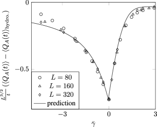
Figure 3: Rescaled deviation of the first cumulant of $A$ particles, $\langle Q_{A}(t)\rangle$, from its deterministic hydrodynamics prediction (11), as a function of $\bar{\gamma}$ (25), for $r_{A}=r_{B}=1/4$. Numerical measurements for systems of $80$ to $320$ sites are compared with our analysis of the critical point (27,28).

VI Critical fluctuations of the current

Let us now discuss the consequences of the slow fluctuations of the first Fourier mode of the density described above on the integrated particle current of $a$ particles, $Q_{a}(t)$. From (13) and (15), we can express the average instantaneous current, $J_{a}$, in terms of $f(\bar{\tau})$ :

$$J_{a}(\tau)=\beta r_{a}(r_{b}-r_{c})+2\beta(r_{b}-r_{c})\sqrt{3\Delta r_{a}r_{b}r_{c}\over\Lambda L}|f(\bar{\tau})|^{2}\\ +{1\over\sqrt{L}}G_{a}(\tau)+{\mathcal{O}}\left(1\over L\right)$$

where $G_{a}$, the space average of the noise $\eta_{a}$, is such that

$$\langle G_{a}(\tau)G_{a}(\tau^{\prime})\rangle=2r_{a}(1-r_{a}){\delta(\tau-\tau^{\prime})}+{\mathcal{O}}(1/\sqrt{L})\,.$$

Therefore, the contributions of the fluctuations of the first Fourier mode $f$ and of the noise $G_{a}$ to $J_{a}$ are of comparable amplitude. The fluctuations of $f$, however, occur on the slower time scale $\bar{\tau}\sim\tau/\sqrt{L}$: hence, they become dominant in the integrated current (I)

$$Q_{a}(t)=L\int_{0}^{t/L^{2}}J_{a}(\tau)d\tau\,,$$

with the $n$-points time correlation function of $f(\bar{\tau})$ giving rise to an anormal growth of the $n$-th cumulant of $Q_{a}$, $\langle Q_{a}^{n}(t)\rangle_{c}$. More precisely, we find that

$$\langle Q_{a}(t)\rangle\simeq{t\over L}\beta r_{a}(r_{c}-r_{b})+{2t\over L^{3/2}}\beta(r_{b}-r_{c})\sqrt{3\Delta r_{a}r_{b}r_{c}\over\Lambda}C_{1}(\bar{\gamma})$$ (27)

and

$$\langle Q_{a}^{n}(t)\rangle_{c}\simeq{t\over L^{5/2-n}}{8\pi^{2}\sqrt{3\Lambda r_{a}r_{b}r_{c}}\over\Delta^{3/2}}\left[\Delta^{3/2}(r_{b}-r_{c})\over 2\pi\Lambda\right]^{n}C_{n}(\bar{\gamma})$$

with $\bar{\gamma}$ as defined in (25) and with

$$C_{n}(\bar{\gamma})=\lim_{\bar{\tau}\to\infty}{1\over\bar{\tau}}\int_{0}^{\bar{\tau}}d\bar{\tau}_{1}..d\bar{\tau}_{n}\langle|f(\bar{\tau}_{1})..f(\bar{\tau}_{n})|^{2}\rangle_{c}$$

a time integral of the $n$-point correlation function of $f(\bar{\tau})$.

Because $f(\bar{\tau})$ follows a Langevin equation in a quartic potential (25), one does not have simple analytical expressions for the $C_{n}(\bar{\gamma})$ for $n\geq 2$. $C_{1}(\bar{\gamma})$, on the other hand, only depends on the stationary average of $|f(\bar{\tau})|^{2}$: since the stationnary state of the Fokker-Planck equation (26) is $P(r,\theta)\propto e^{2\bar{\gamma}r^{2}-r^{4}}$, we obtain easily that

$$C_{1}(\bar{\gamma})=\bar{\gamma}+{1\over 2}{e^{-\bar{\gamma}^{2}}\over\int_{-\infty}^{\bar{\gamma}}e^{-z^{2}}dz}\,.$$ (28)

Thus, we obtain an analytic expression for the deviation of $\langle Q_{A}(t)\rangle$ from its hydrodynamics prediction (11) in the neighborhood of $\beta_{*}$. In Figure 3, we compare this expression to numerical simulations of systems of $80$ to $320$ sites, for $r_{A}=r_{B}=1/4$.

VII Conclusion

In this letter we have seen that a driven diffusive system like the ABC model, at a second order phase transition, may exhibit anomalous Fourier’s law at least for the second and higher cumulants. This is reminiscent of the cumulants of the current which diverge with the system size in the TASEP (the totally asymmetric exclusion process) along the first order transition lineLM2 . The mechanism is however different. Here the large fluctuations can be understood by analysing the dynamics of the first Fourier mode which becomes unstable at the transition whereas, in the TASEP, the large fluctuations of the current are due to the presence of the shock.

The anomalous current fluctuations of the ABC model at the phase transition are accompanied by anomalous long range density fluctuations which can also be understood in terms of the slow noisy dynamics of the first Fourier mode (the density fluctuations will be discussed in the forthcoming longer version of the present letterDG2 ).

An interesting open question would be to compare the anomalous density and the current fluctuations of the ABC model at the transition with those of momentum conserving mechanical models, in particular through the dynamics of their slow modes. Another interesting question would be to study the current fluctuations through other lattice gases (such as an Ising model) when there is coexistence of several phases at equilibrium.

References

• (1) T. Bodineau and B. Derrida, “Current fluctuations in nonequilibrium diffusive systems: an additivity principle,” Phys. Rev. Lett., vol. 92, p. 180601, May 2004.
• (2) L. Bertini, A. De Sole, D. Gabrielli, G. Jona-Lasinio, and C. Landim, “Current fluctuations in stochastic lattice gases,” Phys. Rev. Lett., vol. 94, p. 030601, Jan 2005.
• (3) G. Basile, C. Bernardin, and S. Olla, “Momentum conserving model with anomalous thermal conductivity in low dimensional systems,” Phys. Rev. Lett., vol. 96, p. 204303, May 2006.
• (4) B. Derrida, “Non-equilibrium steady states: fluctuations and large deviations of the density and of the current,” J. Stat. Mech: Theory Exp., no. 07, p. P07023, 2007.
• (5) R. J. Harris and G. M. Schutz, “Fluctuation theorems for stochastic dynamics,” J. Stat. Mech: Theory Exp., no. 07, p. P07020, 2007.
• (6) C. Appert-Rolland, B. Derrida, V. Lecomte, and F. van Wijland, “Universal cumulants of the current in diffusive systems on a ring,” Phys. Rev. E, vol. 78, p. 021122, Aug 2008.
• (7) A. Imparato, V. Lecomte, and F. van Wijland, “Equilibriumlike fluctuations in some boundary-driven open diffusive systems,” Phys. Rev. E, vol. 80, p. 011131, Jul 2009.
• (8) P. I. Hurtado and P. L. Garrido, “Current fluctuations and statistics during a large deviation event in an exactly solvable transport model,” J. Stat. Mech: Theory Exp., no. 02, p. P02032, 2009.
• (9) P. I. Hurtado and P. L. Garrido, “Test of the additivity principle for current fluctuations in a model of heat conduction,” Phys. Rev. Lett., vol. 102, no. 25, p. 250601, 2009.
• (10) S. Prolhac and K. Mallick, “Cumulants of the current in a weakly asymmetric exclusion process,” J. Phys. A: Math. Theor., vol. 42, no. 17, p. 175001, 2009.
• (11) H. Touchette, “The large deviation approach to statistical mechanics,” Phys. Rep., vol. 478, pp. 1 – 69, 2009.
• (12) A. Lazarescu and K. Mallick, “An exact formula for the statistics of the current in the tasep with open boundaries,” J. Phys. A: Math. Theor., vol. 44, p. 315001, 2011.
• (13) H. Lee, L. S. Levitov, and A. Y. Yakovets, “Universal statistics of transport in disordered conductors,” Phys. Rev. B, vol. 51, pp. 4079–4083, Feb 1995.
• (14) C. W. J. Beenakker, “Random-matrix theory of quantum transport,” Rev. Mod. Phys., vol. 69, no. 3, pp. 731–808, 1997.
• (15) Y. M. Blanter and M. Buttiker, “Shot noise in mesoscopic conductors,” Phy. Rep., vol. 336, p. 1, 2000.
• (16) V. Rychkov and M. Büttiker, “Mesoscopic versus macroscopic division of current fluctuations,” Phys. Rev. Lett., vol. 96, no. 16, p. 166806, 2006.
• (17) F. Bonetto, J. L. Lebowitz, and L. Rey-Bellet, “Fourier’s law: a challenge to theorists,” in Mathematical physics 2000, pp. 128–150, London: Imp. Coll. Press, 2000.
• (18) B. Derrida, B. Douçot, and P.-E. Roche, “Current fluctuations in the one-dimensional symmetric exclusion process with open boundaries,” J. Stat. Phys., vol. 115, pp. 717–748, May 2004.
• (19) H. Spohn, Large Scale Dynamics of Interacting Particles. Texts and Monographs in Physics, Springer, November 1991.
• (20) C. Kipnis, C. Marchioro, and E. Presutti, “Heat flow in an exactly solvable model,” J. Stat. Phys., vol. 27, pp. 65–74, Jan 1982.
• (21) L. Bertini, A. Sole, D. Gabrielli, G. Jona-Lasinio, and C. Landim, “Non equilibrium current fluctuations in stochastic lattice gases,” J. Stat. Phys., vol. 123, pp. 237–276, Apr 2006.
• (22) L. Bertini, A. De Sole, D. Gabrielli, G. Jona-Lasinio, and C. Landim, “Towards a nonequilibrium thermodynamics: A self-contained macroscopic description of driven diffusive systems,” J. Stat. Phys., vol. 135, pp. 857–872, 2009.
• (23) B. Li and J. Wang, “Anomalous heat conduction and anomalous diffusion in one-dimensional systems,” Phys. Rev. Lett., vol. 91, p. 044301, Jul 2003.
• (24) T. Mai, A. Dhar, and O. Narayan, “Equilibration and universal heat conduction in Fermi-Pasta-Ulam chains,” Phys. Rev. Lett., vol. 98, p. 184301, May 2007.
• (25) P. Grassberger, W. Nadler, and L. Yang, “Heat conduction and entropy production in a one-dimensional hard-particle gas,” Phys. Rev. Lett., vol. 89, p. 180601, Oct 2002.
• (26) A. Dhar, “Heat conduction in a one-dimensional gas of elastically colliding particles of unequal masses,” Phys. Rev. Lett., vol. 86, pp. 3554–3557, Apr 2001.
• (27) A. Gerschenfeld, B. Derrida, and J. L. Lebowitz, “Anomalous Fourier’s law and long range correlations in a 1D non-momentum conserving mechanical model,” J. Stat. Phys., vol. 141, pp. 757–766, 2010.
• (28) S. Lepri, R. Livi, and A. Politi, “Heat conduction in chains of nonlinear oscillators,” Phys. Rev. Lett., vol. 78, pp. 1896–1899, Mar 1997.
• (29) S. Lepri, R. Livi, and A. Politi, “Thermal conduction in classical low-dimensional lattices,” Phys. Rep., vol. 377, pp. 1–80(80), 2003.
• (30) A. Dhar, “Heat transport in low-dimensional systems,” Adv. Phys., vol. 57, no. 5, pp. 457–537, 2008.
• (31) E. Brunet, B. Derrida, and A. Gerschenfeld, “Fluctuations of the heat flux of a one-dimensional hard particle gas,” EPL, vol. 90, no. 2, p. 20004, 2010.
• (32) M. R. Evans, Y. Kafri, H. M. Koduvely, and D. Mukamel, “Phase separation and coarsening in one-dimensional driven diffusive systems: Local dynamics leading to long-range hamiltonians,” Phys. Rev. E, vol. 58, no. 3, pp. 2764–2778, 1998.
• (33) M. R. Evans, Y. Kafri, H. M. Koduvely, and D. Mukamel, “Phase separation in one-dimensional driven diffusive systems,” Phys. Rev. Lett., vol. 80, no. 3, pp. 425–429, 1998.
• (34) M. Clincy, B. Derrida, and M. R. Evans, “Phase transition in the ABC model,” Phys. Rev. E, vol. 67, no. 6, p. 066115, 2003.
• (35) A. Ayyer, E. Carlen, J. L. Lebowitz, P. Mohanty, D. Mukamel, and E. R. Speer, “Phase diagram of the ABC model on an interval,” J. Stat. Phys., vol. 137, p. 1166, 2009.
• (36) A. Lederhendler and D. Mukamel, “Long-range correlations and ensemble inequivalence in a generalized $abc$ model,” Phys. Rev. Lett., vol. 105, no. 15, p. 150602, 2010.
• (37) J. Barton, J. L. Lebowitz, and E. R. Speer, “The grand canonical ABC model: a reflection asymmetric mean-field Potts model,” J. Phys. A: Math. Theor., vol. 44, no. 6, p. 065005, 2011.
• (38) A. Lederhendler, O. Cohen, and D. Mukamel, “Phase diagram of the ABC model with nonconserving processes,” J. Stat. Mech., no. 11, p. P11016, 2010.
• (39) T. Bodineau and B. Derrida, “Phase fluctuations in the ABC model,” preprint, p. submitted to J. Stat. Phys., 2011.
• (40) L. Bertini, A. D. Sole, D. Gabrielli, G. Jona-Lasinio, and C. Landim, “Stochastic interacting particle systems out of equilibrium,” J. Stat. Mech: Theory Exp., no. 07, p. P07014, 2007.
• (41) A. Gerschenfeld and B. Derrida, “Anormal correlations at a phase transition,” in preparation, 2011.