Functional kernel estimators of large conditional quantiles

Abstract

We address the estimation of conditional quantiles when the covariate is functional and when the order of the quantiles converges to one as the sample size increases. In a first time, we investigate to what extent these large conditional quantiles can still be estimated through a functional kernel estimator of the conditional survival function. Sufficient conditions on the rate of convergence of their order to one are provided to obtain asymptotically Gaussian distributed estimators. In a second time, basing on these result, a functional Weissman estimator is derived, permitting to estimate large conditional quantiles of arbitrary large order. These results are illustrated on finite sample situations.

Keywords: Conditional quantiles, heavy-tailed distributions, functional kernel estimator, extreme-value theory.

AMS 2000 subject classification: 62G32, 62G30, 62E20.

1 Introduction

Let $(X_{i},Y_{i})$, $i=1,\dots,n$ be independent copies of a random pair $(X,Y)$ in $E\times\mathbb{R}$ where $E$ is an infinite dimensional space associated to a semi-metric $d$. We address the problem of estimating $q(\alpha_{n}|x)\in\mathbb{R}$ verifying $\mathbb{P}(Y>q(\alpha_{n}|x)|X=x)=\alpha_{n}$ where $\alpha_{n}\to 0$ as $n\to\infty$ and $x\in E$. In such a case, $q(\alpha_{n}|x)$ is referred to as a large conditional quantile in contrast to classical conditional quantiles (or regression quantiles) for which $\alpha_{n}=\alpha$ is fixed in $(0,1)$. While the nonparametric estimation of ordinary regression quantiles has been extensively studied (see for instance [39, 43] or [20], Chapter 5), less attention has been paid to large conditional quantiles despite their potential interest. In climatology, large conditional quantiles may explain how climate change over years might affect extreme temperatures. In the financial econometrics literature, they illustrate the link between extreme hedge fund returns and some measures of risk. Parametric models are introduced in [10, 42] and semi-parametric methods are considered in [2, 34]. Fully non-parametric estimators have been first introduced in [9, 6] through local polynomial and spline models. In both cases, the authors focus on univariate covariates and on the finite sample properties of the estimators. Nonparametric methods based on moving windows and nearest neighbors are introduced respectively in [25] and [26]. We also refer to [15], Theorem 3.5.2, for the approximation of the nearest neighbors distribution using the Hellinger distance and to [21] for the study of their asymptotic distribution.

An important literature is devoted to the particular case where the conditional distribution of $Y$ given $X=x$ has a finite endpoint $\varphi(x)$ and when $X$ is a finite dimensional random variable. The function $\varphi$ is referred to as the frontier and can be estimated from an estimator of the conditional quantile $q(\alpha_{n}|x)$ with $\alpha_{n}\to 0$. As an example, a kernel estimator of $\varphi$ is proposed in [29], the asymptotic normality being proved only when $Y$ given $X=x$ is uniformly distributed on $[0,\varphi(x)]$. We refer to [36] for a review on this topic.

Estimation of unconditional large quantiles is also widely studied since the introduction of Weissman estimator [45] dedicated to heavy-tailed distributions, Weibull-tail estimators [12, 24] dedicated to light-tailed distributions and Dekkers and de Haan estimator [11] adapted to the general case.

In this paper, we focus on the setting where the conditional distribution of $Y$ given $X=x$ has an infinite endpoint and is heavy-tailed, an analytical characterization of this property being given in the next section. In such a case, the frontier function does not exist and $q(\alpha_{n}|x)\to\infty$ as $\alpha_{n}\to 0$. Nevertheless, we show, under some conditions, that large regression quantiles $q(\alpha_{n}|x)$ can still be estimated through a functional kernel estimator of $\mathbb{P}(Y>.|x)$. We provide sufficient conditions on the rate of convergence of $\alpha_{n}$ to 0 so that our estimator is asymptotically Gaussian distributed. Making use of this, some functional estimators of the conditional tail-index are introduced and a functional Weissman estimator [45] is derived, permitting to estimate large conditional quantiles $q(\beta_{n}|x)$ where $\beta_{n}\to 0$ arbitrarily fast.

Assumptions are introduced and discussed in Section 2. Main results are provided in Section 3 and illustrated both on simulated and real data in Section 4 and Section 5. Extensions of this work are briefly discussed in Section 6. Proofs are postponed to the appendix.

2 Notations and assumptions

The conditional survival function (csf) of $Y$ given $X=x$ is denoted by $\bar{F}(y|x)=\mathbb{P}(Y>y|X=x)$. The functional estimator of $\bar{F}(y|x)$ is defined for all $(x,y)\in E\times\mathbb{R}$ by

$$\hat{\bar{F_{n}}}(y|x)=\left.\sum_{i=1}^{n}K(d(x,X_{i})/h)Q((Y_{i}-y)/\lambda)\right/\sum_{i=1}^{n}K(d(x,X_{i})/h),$$ (1)

with $Q(t)=\int_{-\infty}^{t}Q^{\prime}(s)ds$ where $K:\mathbb{R}^{+}\to\mathbb{R}^{+}$ and $Q^{\prime}:\mathbb{R}\to\mathbb{R}^{+}$ are two kernel functions, and $h=h_{n}$ and $\lambda=\lambda_{n}$ are two nonrandom sequences (called window-width) such that $h\to 0$ as $n\to\infty$. Let us emphasize that the condition $\lambda\to 0$ is not required in this context. This estimator was considered for instance in [20], page 56. Its rate of uniform strong consistency is established by [16]. In Theorem 1 hereafter, the asymptotic distribution of (1) is established when estimating small tail probabilities, i.e when $y=y_{n}$ goes to infinity with the sample size $n$. Similarly, the functional estimators of conditional quantiles $q(\alpha|x)$ are defined via the generalized inverse of $\hat{\bar{F_{n}}}(.|x)$:

$$\hat{q}_{n}(\alpha|x)=\hat{\bar{F_{n}}}^{\leftarrow}(\alpha|x)=\inf\{t,\;\hat{\bar{F_{n}}}(t|x)\leq\alpha\},$$ (2)

for all $\alpha\in(0,1)$. Many authors are interested in this estimator for fixed $\alpha\in(0,1)$. Weak and strong consistency are proved respectively in [43] and [22]. Asymptotic normality is shown in [3, 40, 44] when $E$ is finite dimensional and by [18] for a general metric space under dependence assumptions. In Theorem 2, the asymptotic distribution of (2) is investigated when estimating large quantiles, i.e when $\alpha=\alpha_{n}$ goes to 0 as the sample size $n$ goes to infinity. The asymptotic behavior of such estimators depends on the nature of the conditional distribution tail. In this paper, we focus on heavy tails. More specifically, we assume that the csf satisfies

(A.1): $\displaystyle\bar{F}(y|x)=c(x)\exp\left\{-\int_{1}^{y}\left(\frac{1}{\gamma(x)}-\varepsilon(u|x)\right)\frac{du}{u}\right\}$,

where $\gamma$ is a positive function of the covariate $x$, $c$ is a positive function and $|\varepsilon(.|x)|$ is continuous and ultimately decreasing to 0. Examples of such distributions are provided in Table 1. (A.1) implies that the conditional distribution of $Y$ given $X=x$ is in the Fréchet maximum domain of attraction. In this context, $\gamma(x)$ is referred to as the conditional tail-index since it tunes the tail heaviness of the conditional distribution of $Y$ given $X=x$. More details on extreme-value theory can be found for instance in [14]. Assumption (A.1) also yields that $\bar{F}(.|x)$ is regularly varying at infinity with index $-1/\gamma(x)$. i.e for all $\zeta>0$,

$$\lim_{y\to\infty}\frac{\bar{F}(\zeta y|x)}{\bar{F}(y|x)}=\zeta^{-1/\gamma(x)}.$$ (3)

We refer to [4] for a general account on regular variation theory. The auxiliary function $\varepsilon(.|x)$ plays an important role in extreme-value theory since it drives the speed of convergence in (3) and more generally the bias of extreme-value estimators. Therefore, it may be of interest to specify how it converges to 0. In [1, 31], $|\varepsilon(.|x)|$ is supposed to be regularly varying and the estimation of the corresponding regular variation index is addressed.

Some Lipschitz conditions are also required:

(A.2): There exist $\kappa_{\varepsilon}$, $\kappa_{c}$, $\kappa_{\gamma}>0$ and $u_{0}>1$ such that for all $(x,x^{\prime})\in E\times E$ and $u>u_{0}$,

$$\displaystyle\left|\log c(x)-\log c(x^{\prime})\right| \leq \kappa_{c}d(x,x^{\prime}),$$

$$\displaystyle\left|\varepsilon(u|x)-\varepsilon(u|x^{\prime})\right| \leq \kappa_{\varepsilon}d(x,x^{\prime}),$$

$$\displaystyle\left|\frac{1}{\gamma(x)}-\frac{1}{\gamma(x^{\prime})}\right| \leq \kappa_{\gamma}d(x,x^{\prime}).$$

The last two assumptions are standard in the functional kernel estimation framework.

(A.3): $K$ is a function with support $[0,1]$ and there exist $0<C_{1}<C_{2}<\infty$ such that $C_{1}\leq K(t)\leq C_{2}$ for all $t\in[0,1]$.

(A.4): $Q^{\prime}$ is a probability density function (pdf) with support $[-1,1]$.

One may also assume without loss of generality that $K$ integrates to one. In this case, $K$ is called a type I kernel, see [20], Definition 4.1. Letting $B(x,h)$ be the ball of center $x$ and radius $h$, we finally introduce $\varphi_{x}(h):=\mathbb{P}(X\in B(x,h)$ the small ball probability of $X$. Under (A.3), the $\tau$-th moment $\mu^{(\tau)}_{x}(h):=\mathbb{E}\{K^{\tau}(d(x,X)/h)$ can be controlled for all $\tau>0$ by Lemma 3 in Appendix. It is shown that $\mu^{(\tau)}_{x}(h)$ is of the same asymptotic order as $\varphi_{x}(h)$.

3 Main results

The first step towards the estimation of large conditional quantiles is the estimation of small tail probabilities $\bar{F}(y_{n}|x)$ when $y_{n}\to\infty$ as $n\to\infty$.

3.1 Estimation of small tail probabilities

Defining

$$\Lambda_{n}(x)=\left(n\bar{F}(y_{n}|x)\frac{(\mu_{x}^{(1)}(h))^{2}}{\mu_{x}^{(2)}(h)}\right)^{-1/2},$$

the following result provides sufficient conditions for the asymptotic normality of $\hat{\bar{F_{n}}}(y_{n}|x)$.

Theorem 1

Suppose (A.1) – (A.4) hold. Let $x\in E$ such that $\varphi_{x}(h)>0$ and introduce $y_{n,j}=a_{j}y_{n}(1+o(1))$ for $j=1,\dots,J$ with $0<a_{1}<a_{2}<\dots<a_{J}$ and where $J$ is a positive integer. If $y_{n}\to\infty$ such that $n\varphi_{x}(h)\bar{F}(y_{n}|x)\to\infty$ and $n\varphi_{x}(h)\bar{F}(y_{n}|x)(\lambda/y_{n}\vee h\log y_{n})^{2}\to 0$ as $n\to\infty$, then

$$\left\{\Lambda_{n}^{-1}(x)\left(\frac{\hat{\bar{F_{n}}}(y_{n,j}|x)}{\bar{F}(y_{n,j}|x)}-1\right)\right\}_{j=1,\dots,J}$$

is asymptotically Gaussian, centered, with covariance matrix $C(x)$ where $C_{j,j^{\prime}}(x)=a^{1/\gamma(x)}_{j\wedge j^{\prime}}$ for $(j,j^{\prime})\in\{1,\dots,J\}^{2}$.

Note that $n\varphi_{x}(h)\bar{F}(y_{n}|x)\to\infty$ is a necessary and sufficient condition for the almost sure presence of at least one sample point in the region $B(x,h)\times(y_{n},\infty)$ of $E\times\mathbb{R}$, see Lemma 4 in Appendix. Thus, this natural condition states that one cannot estimate small tail probabilities out of the sample using $\hat{\bar{F_{n}}}$. Besides, from Lemma 3, $\Lambda_{n}^{-2}(x)$ is of the same asymptotic order as $n\varphi_{x}(h)\bar{F}(y_{n}|x)$ and consequently $\Lambda_{n}(x)\to 0$ as $n\to\infty$. Theorem 1 thus entails $\hat{\bar{F_{n}}}(y_{n,j}|x)/\bar{F}(y_{n,j}|x)\stackrel{{\scriptstyle P}}{{\longrightarrow}}1$ which can be read as a consistency of the estimator. The second condition $n\varphi_{x}(h)\bar{F}(y_{n}|x)(\lambda/y_{n}\vee h\log y_{n})^{2}\to 0$ imposes to the biases $\lambda/y_{n}$ and $h\log y_{n}$ introduced by the two smoothings to be negligible compared to the standard deviation $\Lambda_{n}(x)$ of the estimator. Theorem 1 may be compared to [13] which establishes the asymptotic behavior of the empirical survival function in the unconditional case but without assumption on the distribution.

3.2 Estimation of large conditional quantiles within the sample

In this paragraph, we focus on the estimation of large conditional quantiles of order $\alpha_{n}$ such that $n\varphi_{x}(h)\alpha_{n}\to\infty$ as $n\to\infty$. This is a necessary and sufficient condition for the almost sure presence of at least one sample point in the region $B(x,h)\times(q(\alpha_{n}|x),\infty)$ of $E\times\mathbb{R}$, see Lemma 4 in Appendix. In other words, the large conditional quantile $q(\alpha_{n}|x)$ is located within the sample. Letting

$$\sigma_{n}(x)=\left(n\alpha_{n}\frac{(\mu_{x}^{(1)}(h))^{2}}{\mu_{x}^{(2)}(h)}\right)^{-1/2},$$

Lemma 3 shows that $\sigma_{n}(x)$ is of the same asymptotic order as $(n\varphi_{x}(h)\alpha_{n})^{-1/2}$ and thus the condition $n\varphi_{x}(h)\alpha_{n}\to\infty$ is equivalent to $\sigma_{n}(x)\to 0$ as $n\to\infty$.

Theorem 2

Suppose (A.1) – (A.4) hold. Let $x\in E$ such that $\varphi_{x}(h)>0$ and consider a sequence $\tau_{1}>\tau_{2}>\dots>\tau_{J}>0$ where $J$ is a positive integer. If $\alpha_{n}\to 0$ such that $\sigma_{n}(x)\to 0$ and $\sigma_{n}^{-1}(x)(\lambda/q(\alpha_{n}|x)\vee h\log\alpha_{n})\to 0$ as $n\to\infty$, then

$$\left\{\sigma_{n}^{-1}(x)\left(\frac{\hat{q}_{n}(\tau_{j}\alpha_{n}|x)}{q(\tau_{j}\alpha_{n}|x)}-1\right)\right\}_{j=1,\dots,J}$$

is asymptotically Gaussian, centered, with covariance matrix ${\gamma^{2}(x)}\Sigma$ where $\Sigma_{j,j^{\prime}}=1/\tau_{j\wedge j^{\prime}}$ for $(j,j^{\prime})\in\{1,\dots,J\}^{2}$.

Remark that (A.1) provides an asymptotic expansion of the density function of $Y$ given $X=x$:

$$f(y|x)=\frac{1}{\gamma(x)}\frac{\bar{F}(y|x)}{y}(1-\varepsilon(y|x))=\frac{1}{\gamma(x)}\frac{\bar{F}(y|x)}{y}(1+o(1))$$

as $y\to\infty$. Consequently, Theorem 2 entails that the random vector

$$\left\{\frac{\mu_{x}^{(1)}(h)}{(\mu_{x}^{(2)}(h))^{1/2}}(n\tau_{j}\alpha_{n}(1-\tau_{j}\alpha_{n}))^{-1/2}f(q(\tau_{j}\alpha_{n}|x)|x)\left(\hat{q}_{n}(\tau_{j}\alpha_{n}|x)-q(\tau_{j}\alpha_{n}|x)\right)\right\}_{j=1,\dots,J}$$

is also asymptotically Gaussian and centered. This result coincides with [3], Theorem 6.4 established in the case where $\alpha_{n}=\alpha$ is fixed in $(0,1)$ and in a finite dimensional setting.

3.3 Estimation of arbitrary large conditional quantiles

This paragraph is dedicated to the estimation of large conditional quantiles of arbitrary small order $\beta_{n}$. For instance, if $n\varphi_{x}(h)\beta_{n}\to c\in[1,\infty)$ then $q(\beta_{n}|x)$ is located near the boundary of the sample. If $n\varphi_{x}(h)\beta_{n}\to c\in[0,1)$ then $q(\beta_{n}|x)$ is located outside the sample. Here, a functional Weissman estimator [45] is proposed to tackle all possible situations:

$$\hat{q}_{n}^{\mbox{\tiny W}}(\beta_{n}|x)=\hat{q}_{n}(\alpha_{n}|x)(\alpha_{n}/\beta_{n})^{\hat{\gamma}_{n}(x)}.$$ (4)

Here, $\hat{q}_{n}(\alpha_{n}|x)$ is the functional estimator (2) of a large conditional quantile $q(\alpha_{n}|x)$ within the sample and $\hat{\gamma}_{n}(x)$ is an estimator of the conditional tail-index $\gamma(x)$. As illustrated in the next theorem, the extrapolation factor $(\alpha_{n}/\beta_{n})^{\hat{\gamma}_{n}(x)}$ allows to estimate arbitrary large quantiles.

Theorem 3

Suppose (A.1) – (A.4) hold. Let $x\in E$ and introduce

• $\alpha_{n}\to 0$ such that $\sigma_{n}(x)\to 0$ and $\sigma_{n}^{-1}(x)(\lambda/q(\alpha_{n}|x)\vee h\log\alpha_{n}\vee\varepsilon(q(\alpha_{n}|x)|x))\to 0$ as $n\to\infty$,

• $(\beta_{n})$ such that $\beta_{n}/\alpha_{n}\to 0$ as $n\to\infty$,

• $\hat{\gamma}_{n}(x)$ such that $\sigma_{n}^{-1}(x)(\hat{\gamma}_{n}(x)-\gamma(x))\stackrel{{\scriptstyle d}}{{\longrightarrow}}{\mathcal{N}}(0,V(x))$ where $V(x)>0$.

Then,

$$\frac{\sigma_{n}^{-1}(x)}{\log(\alpha_{n}/\beta_{n})}\left(\frac{\hat{q}_{n}^{\mbox{\tiny W}}(\beta_{n}|x)}{q(\beta_{n}|x)}-1\right)\stackrel{{\scriptstyle d}}{{\longrightarrow}}{\mathcal{N}}(0,V(x)).$$

Let us now focus on the estimation of the conditional tail-index. Let $\alpha_{n}\to 0$ and consider a sequence $1=\tau_{1}>\tau_{2}>\dots>\tau_{J}>0$ where $J$ is a positive integer. Two additional notations are introduced for the sake of simplicity: $u=(1,\dots,1)^{t}\in\mathbb{R}^{J}$ and $v=(\log(1/\tau_{1}),\dots,\log(1/\tau_{J}))^{t}\in\mathbb{R}^{J}$. The following family of estimators is proposed

$$\hat{\gamma}^{\phi}_{n}(x)=\frac{\phi(\log\hat{q}_{n}(\tau_{1}\alpha_{n}|x),\dots,\log\hat{q}_{n}(\tau_{J}\alpha_{n}|x))}{\phi(\log(1/\tau_{1}),\dots,\log(1/\tau_{J}))},$$ (5)

where $\phi:\mathbb{R}^{J}\to\mathbb{R}$ denotes a twice differentiable function verifying the shift and location invariance conditions

$$\left\{\begin{array}[]{lll}\phi(\theta v)&=&\theta\phi(v)\\ \phi(\eta u+x)&=&\phi(x)\end{array}\right.$$ (6)

for all $\theta>0$, $\eta\in\mathbb{R}$ and $x\in\mathbb{R}^{J}$. In the case where $J=3$, $\tau_{1}=1$, $\tau_{2}=1/2$ and $\tau_{3}=1/4$, the function

$$\phi_{\mbox{\tiny FP}}(x_{1},x_{2},x_{3})=\log\left(\frac{\exp(4x_{2})-\exp(4x_{1})}{\exp(4x_{3})-\exp(4x_{2})}\right)$$

leads us to a functional version of Pickands estimator [38]:

$$\hat{\gamma}_{n}^{\phi_{\mbox{\tiny FP}}}(x)=\frac{1}{\log 2}\log\left(\frac{\hat{q}_{n}(\alpha_{n}|x)-\hat{q}_{n}(2\alpha_{n}|x)}{\hat{q}_{n}(2\alpha_{n}|x)-\hat{q}_{n}(4\alpha_{n}|x)}\right).$$

We refer to [28] for a different variant of Pickands estimator in the context where the distribution of $Y$ given $X=x$ has a finite endpoint. Besides, introducing the function $m_{p}(x_{1},\dots,x_{J})=\sum_{j=1}^{J}(x_{j}-x_{1})^{p}$ for all $p>0$ and considering $\phi_{p}(x)=m_{p}^{1/p}(x)$ gives rise to a functional version of the estimator considered for instance in [41], example (a):

$$\hat{\gamma}^{\phi_{p}}_{n}(x)=\left(\sum_{j=1}^{J}\left[\log\hat{q}_{n}(\tau_{j}\alpha_{n}|x)-\log\hat{q}_{n}(\alpha_{n}|x)\right]^{p}\left/\sum_{j=1}^{J}[\log(1/\tau_{j})]^{p}\right.\right)^{1/p}.$$

As a particular case $\phi_{1}(x)=m_{1}(x)$ corresponds to a functional version of the Hill estimator [35]:

$$\hat{\gamma}_{n}^{\phi_{1}}(x)=\sum_{j=1}^{J}\left[\log\hat{q}_{n}(\tau_{j}\alpha_{n}|x)-\log\hat{q}_{n}(\alpha_{n}|x)\right]\left/\sum_{j=1}^{J}\log(1/\tau_{j})\right..$$

More interestingly, if $\{\phi^{(1)},\dots,\phi^{(H)}\}$ is a set of $H$ functions satisfying (6) and if $A:\mathbb{R}^{H}\to\mathbb{R}$ is a homogeneous function of degree 1, then the aggregated function $A(\phi^{(1)},\dots,\phi^{(H)})$ also satisfies (6). Generalizations of the functional Hill estimator can then be obtained using $H=2$, $A_{p}(x,y)=x^{p}y^{1-p}$ and defining $\phi_{p,q,r}=A_{p}(\phi_{q},\phi_{r})=m_{q}^{p/q}m_{r}^{(1-p)/r}$:

$$\hat{\gamma}^{\phi_{p,q,r}}_{n}(x)=\frac{\left(\sum_{j=1}^{J}\left[\log\hat{q}_{n}(\tau_{j}\alpha_{n}|x)-\log\hat{q}_{n}(\alpha_{n}|x)\right]^{p}\right)^{p/q}\left(\sum_{j=1}^{J}[\log(1/\tau_{j})]^{r}\right)^{(p-1)/r}}{\left(\sum_{j=1}^{J}\left[\log\hat{q}_{n}(\tau_{j}\alpha_{n}|x)-\log\hat{q}_{n}(\alpha_{n}|x)\right]^{r}\right)^{(p-1)/r}\left(\sum_{j=1}^{J}[\log(1/\tau_{j})]^{p}\right)^{p/q}}.$$

For instance, the estimator introduced by [32], equation (2.2) corresponds to the particular function $\phi_{p,p,1}$ and the estimator of [5] corresponds to $\phi_{p,p\theta,p-1}$.

For an arbitrary function $\phi$, the asymptotic normality of $\hat{\gamma}^{\phi}_{n}(x)$ is a consequence of Theorem 2. The following result permits to establish the asymptotic normality of the above mentioned estimators in an unified way.

Theorem 4

Under the assumptions of Theorem 2 and if, moreover, $\sigma_{n}^{-1}(x)\varepsilon(q(\alpha_{n}|x)|x)\to 0$ as $n\to\infty$, then, $\sigma_{n}^{-1}(x)(\hat{\gamma}^{\phi}_{n}(x)-\gamma(x))$ converges to a centered Gaussian random variable with variance

$$V_{\phi}(x)=\frac{\gamma^{2}(x)}{\phi^{2}(v)}(\nabla\phi(\gamma(x)v))^{t}\Sigma(\nabla\phi(\gamma(x)v)).$$

Let us note that the additional condition $\sigma_{n}^{-1}(x)\varepsilon(q(\alpha_{n}|x)|x)\to 0$ is standard in the extreme-value framework: Neglecting the unknown function $\varepsilon(.|x)$ in the construction of $\hat{\gamma}^{\phi}_{n}(x)$ yields a bias that should be negligible with respect to the standard deviation $\sigma_{n}(x)$ of the estimator. Finally, combining Theorem 3 and Theorem 4, the asymptotic distribution of the functional large quantile estimator $\hat{q}_{n}^{\mbox{\tiny W},\phi}(\beta_{n}|x)$ based on (4) and (5) is readily obtained.

Corollary 1

Suppose (A.1) – (A.4) hold. Let $x\in E$ such that $\varphi_{x}(h)>0$ and consider a sequence $1=\tau_{1}>\tau_{2}>\dots>\tau_{J}>0$ where $J$ is a positive integer. If

• $\alpha_{n}\to 0$, $\sigma_{n}(x)\to 0$ and $\sigma_{n}^{-1}(x)(\lambda/q(\alpha_{n}|x)\vee h\log\alpha_{n}\vee\varepsilon(q(\alpha_{n}|x)|x))\to 0$ as $n\to\infty$,

• $\beta_{n}/\alpha_{n}\to 0$ as $n\to\infty$,

then

$$\frac{\sigma_{n}^{-1}(x)}{\log(\alpha_{n}/\beta_{n})}\left(\frac{\hat{q}_{n}^{\mbox{\tiny W},\phi}(\beta_{n}|x)}{q(\beta_{n}|x)}-1\right)\stackrel{{\scriptstyle d}}{{\longrightarrow}}{\mathcal{N}}(0,V_{\phi}(x)).$$

As an example, in the case of the functional Hill and Pickands estimators, we obtain

$$V_{\phi_{1}}(x) = \gamma^{2}(x)\left(\sum_{j=1}^{J}\frac{2(J-j)+1}{\tau_{j}}-J^{2}\right)\left/\left(\sum_{j=1}^{J}\log(1/\tau_{j})\right)^{2}\right..$$

$$V_{\phi_{\mbox{\tiny FP}}}(x) = \frac{\gamma^{2}(x)(2^{2\gamma(x)+1}+1)}{4(\log 2)^{2}(2^{\gamma(x)}-1)^{2}}.$$

Clearly, $V_{\phi_{\mbox{\tiny FP}}}(x)$ is the variance of the classical Pickands estimator, see for instance [33], Theorem 3.3.5.

4 Illustration on simulated data

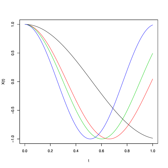
Figure 1: Four realizations of the random function $X(.)$.

The finite sample performance is illustrated on $N=200$ replications of a sample of size $n=500$ from a random pair $(X,Y)$, where the functional covariate $X\in E=L^{2}[0,1]$ is defined by $X(t)=\cos(2\pi Zt)$ for all $t\in[0,1]$ where $Z$ is uniformly distributed on $[1/4,1]$. Some examples of simulated random functions $X$ are depicted on Figure 1. Besides, the conditional distribution of $Y$ given $X$ is a Burr distribution (see Table 1) with parameters $\tau(X)=2$ and $\lambda(X)=2/(8\|X\|_{2}^{2}-3)$ with

$$\|X\|_{2}^{2}=\int_{0}^{1}X^{2}(t)dt=\frac{1}{2}\left(1+\frac{\sin(4\pi Z)}{4\pi Z}\right).$$

We focus on the estimation of $q(\beta_{n}|x)$ with $\beta_{n}=5/n$. To this end, the functional Weissman estimator $\hat{q}_{n}^{\mbox{\tiny W}}(\beta_{n}|x)$ is used with a piecewise linear kernel $K(t)=(1.9-1.8t)\mathbb{I}\{t\in[0,1]\}$ and the triangular kernel $Q^{\prime}$. The conditional tail index is estimated by the functional Hill estimator ${\hat{\gamma}}_{n}^{\phi_{1}}$. The choice of the semi-metric $d$ is a recurrent issue in functional estimation (see [20], Chapter 3). Here, two semi-metrics are considered. The first one is defined for all $(s,t)\in E^{2}$ by $d_{X}(s,t)=\|s-t\|_{2}$ and coincides with the $L_{2}$ distance between functions. Remarking that the conditional quantile $q(\alpha_{n}|X)$ depends only on $\|X\|^{2}_{2}$, or equivalently on $Z$, another interesting semi-metric is $d_{Z}(s,t)=\left|\|s\|_{2}^{2}-\|t\|_{2}^{2}\right|$. Finally, in Section 5, an example of the use of a metric based on second derivatives is presented.

With such choices, the functional Weissman estimator $\hat{q}_{n}^{\mbox{\tiny W}}(\beta_{n}|x)$ depends on three parameters $h$, $\lambda$ and $\alpha_{n}$ and on the $\tau_{j}$’s used to compute ${\hat{\gamma}}_{n}^{\phi_{1}}$.

- The smoothing parameter $h$ is selected using the cross-validation approach introduced in [46] and implemented for instance in [8, 23]:

$$h^{opt}=\arg\min\left\{\sum^{n}_{i=1}\sum^{n}_{j=1}\left(\mathbb{I}{\{Y_{i}\geq Y_{j}\}}-{\hat{\bar{F_{n}}}}_{,-i}(Y_{j}|X_{i})\right)^{2},\ h\in{\cal H}\right\}$$

where ${\hat{\bar{F_{n}}}}_{,-i}$ is the estimator (depending on $h$) given in (1) computed from the sample $\{(X_{\ell},Y_{\ell}),~{}1\leq\ell\leq n,~{}\ell\neq i\}$. Here, ${\cal H}$ is a regular grid, ${\cal H}=\{h_{1}\leq h_{2}\leq\dots\leq h_{M}\}$ with $h_{1}=1/100$, $h_{M}=1/10$ and $M=20$. Let us note that this approach was originally proposed for finite dimensional covariates. Up to our knowledge, its optimality (with respect to the mean integrated squared error for instance) is not established in the functional framework. We refer to [17] for such a work in functional regression.
- In our experiments, the choice of the bandwidth $\lambda$ appeared to be less crucial than the other smoothing parameter $h$. It could have been selected with the same criteria as previously, but for simplicity reasons, it has been fixed to $\lambda=0.1$.
- The choice of $\alpha_{n}$ is equivalent to the choice of the number of upper order statistics in the non-conditional extreme-value theory. It is still an open question, even though some techniques have been proposed, see for instance [7] for a bootstrap based method.
- The selection of the $\tau_{j}$’s is equivalent to the selection of an estimator for the conditional tail index. Once again, extreme-value theory does not provide optimal solution to this problem.

In order to assess the impact of the choice of $\alpha_{n}$ and $\tau_{j}$’s, the $L_{2}$-errors

$$\Delta_{d}^{(r)}=\sum_{i=1}^{n}\left(\hat{q}_{n}^{\mbox{\tiny W}}(\beta_{n}|X_{i})^{(r)}-q(\beta_{n}|X_{i})\right)^{2},$$

$r=1,\dots,N$ have been computed. Here, $\hat{q}_{n}^{\mbox{\tiny W}}(\beta_{n}|X_{i})^{(r)}$ is the estimation computed on the $r$th replication and $d$ can be either $d_{X}$ or $d_{Z}$. Different values of $\alpha_{n}$ and $\tau_{j}$ are investigated: $\alpha_{n}=c\log(n)/n$ with $c\in\{5,10,15,20\}$ and $\tau_{j}=(1/j)^{s}$ with $s\in\{1,2,3,10\}$. The median, 10% quantile and 90% quantile of the $\Delta_{d}^{(r)}$ errors are collected in Table 2. For a fixed value of $s$, the best error obtained with the semi-metric $d_{Z}$ is always smaller than the best error obtained with $d_{X}$ (both displayed in bold font). Let us note that the optimal value of $c$ does not seem to depend on the semi-metric. Besides, it will appear in the following that the estimations are not, at least visually, very sensitive with respect to the choice of $\alpha_{n}$ (or equivalently $c$) and $\tau_{j}$ (or equivalently $s$). In Figure 2–4, the estimator $\hat{q}_{n}^{\mbox{\tiny W}}(\beta_{n}|x)$ is represented as a function of $Z$. The estimator has been computed for two sets of ($\alpha_{n}$, $\tau_{j}$): ($\alpha_{n}=15\log(n)/n$, $\tau_{j}=(1/j)^{3}$) and ($\alpha_{n}=10\log(n)/n$, $\tau_{j}=(1/j)^{2}$) and for the two semi-metrics $d_{X}$ and $d_{Z}$. We limited ourselves to the representation of the estimator computed on the replications giving rise to the median, 10% quantile and 90% quantile of the $L_{2}$-errors $\Delta_{d}^{(r)}$, $r=1,\dots,N$. It appears that there is no visual significative difference between the two choices of ($\alpha_{n}$, $\tau_{j}$).

5 Illustration on real data

In this section, we propose to illustrate the behaviour of our large conditional quantiles estimators on functional chemometric data. It concerns $n=215$ samples of finely chopped meat (see for example [19] for more details). For each unit $i$ taken among this sample, we observe one spectrometric curve $\chi_{i}$ discretized at 100 wavelengths $\lambda_{1},\ldots,\lambda_{100}$. The covariate $x_{i}$ is thus defined by $x_{i}=(x_{i,1},\dots,x_{i,100})^{t}$ with $x_{i,j}=\chi_{i}(\lambda_{j})$ for all $j=1,\dots,100$. Each variable $x_{i,j}$ is the $-\log_{10}$ of the transmittance recorded by the Tecator Infratec Food and Feed Analyzer spectrometer. The dataset can be found at http://lib.stat.cmu.edu/datasets/tecator.

Clearly, the covariate $x_{i}$ is in fact a discretized curve but, as mentioned in [37], the fineness of the grid spanning the discretization allows us to consider each subject as a continuous curve. Hence, the covariate can be considered as belonging to an infinite dimensional space $E$. For each spectrometric curve $\chi_{i}$, the fat content ${\tilde{Y}}_{i}\in[0,100]$ (in percentage) is given. Since these values are bounded they cannot satisfy model (A.1) and we propose to use as variable of interest the inverse of the fat content defined as: $Y_{i}=100/{\tilde{Y}}_{i}\in[1,\infty)$, $i=1,\ldots,n$.

In the following, the semi-metric based on the second derivative is adopted, as advised in [20], Chapter 9:

$$d^{2}(\chi_{i},\chi_{j})=\int\left(\chi_{i}^{(2)}(t)-\chi_{j}^{(2)}(t)\right)^{2}dt,$$

where $\chi^{(2)}$ denotes the second derivative of $\chi$. To compute this semi-metric, one can use an approximation of the functions $\chi_{i}$ and $\chi_{j}$ based on B-splines as proposed in [20], Chapter 3. Here, we limit ourselves to a discretized version $\tilde{d}$ of $d$:

$$\tilde{d}^{2}(x_{i},x_{j})=\sum_{l=2}^{99}\left\{(x_{i,l+1}-x_{j,l+1})+(x_{i,l-1}-x_{j,l-1})-2(x_{i,l}-x_{j,l})\right\}^{2}.$$

Other semi-metrics could be considered: Functional Principal Component Analysis (FPCA) or Multivariate Partial Least-Squares Regression (MPLSR) are useful tools for computing proximities between curves in reduced dimensional spaces, see [20], Section 3.4.

We propose to estimate the large conditional quantile of order $\beta_{n}=5/n$ in a given direction of the space $E$. More precisely, we focus on the segment $[\chi_{i_{0}},\chi_{i_{1}}]$ where $\chi_{i_{0}}$ and $\chi_{i_{1}}$ denote the most different curves in the sample, i.e.

$$(i_{0},i_{1})=\arg\max_{1\leq i<j\leq n}\tilde{d}(x_{i},x_{j}).$$

The selected curves $\chi_{i_{0}}$ and $\chi_{i_{1}}$ are plotted in Figure 5. Since these curves appear to be smooth, the chosen semi-metric, which is based on the second derivative, seems to be well adapted. The conditional quantile to estimate is $q(\beta_{n},t(\xi))$ where $t(\xi)=\xi\chi_{i_{1}}+(1-\xi)\chi_{i_{0}}$ for $\xi\in[0,1]$. To this end, the functional Weissman estimator is considered with the same kernels as in the previous section. The selected smoothing parameters are $h=0.02$ and $\lambda=0.1$.

The estimated quantile $\hat{q}_{n}^{\mbox{\tiny W}}(\beta_{n},t(\xi))$ is plotted as a function of $\xi$ in Figure 6 for different values of weights $\tau_{j}$ and probability $\alpha_{n}$. Here again, it appears that the estimated quantiles are not too sensitive with respect to these parameters. The globally decreasing shape of the curves indicates that heaviest tails (i.e. largest values of $\gamma(t(\xi))$) are found in the neighbourhood of the curve $\chi_{i_{0}}$ (i.e. for small values of $\xi$). At the opposite, lightest tails are found in the neighbourhood of the curve $\chi_{i_{1}}$. These results are confirmed by Figure 7: The estimated conditional tail-index $\hat{\gamma}_{n}^{\phi_{1}}(x)$ is larger for $x=\chi_{i_{0}}$ than for $x=\chi_{i_{1}}$. These very different shapes confirm a strong heterogeneity of the sample in terms of tail behaviour.

6 Further work

Our further work will consist in establishing uniform convergence results. The rate of uniform strong consistency of the csf estimator $\hat{\bar{F_{n}}}(y|x)$ defined in (1) is already known since [16] for fixed $y$. The first step will then to adapt this result for $y=y_{n}\to\infty$ as $n\to\infty$. On this basis, it should be possible to get uniform results for $\hat{q}(\alpha_{n}|x)$ (see (2)) in the case of large conditional quantiles withing the sample, ie. $\alpha_{n}\to 0$ with $n\varphi_{x}(x)\alpha_{n}\to\infty$. The last step would be to extend these results to $\hat{q}_{n}^{\mbox{\tiny W}}(\beta_{n}|x)$ defined in (4) when $\beta_{n}\to 0$ arbitrarily fast. Such results would require the uniform convergence of $\hat{\gamma}_{n}(x)$, the estimator of the conditional tail index.

7 Appendix: Proofs

7.1 Preliminary results

The following two lemmas are of analytical nature. The first one is dedicated to the control of the local variations of the csf when the quantity of interest $y$ goes to infinity.

Lemma 1

Let $x\in E$ and suppose (A.1) and (A.2) hold.
(i) If $y_{n}\to\infty$ and $h\log y_{n}\to 0$ as $n\to\infty$, then, for $n$ large enough,

$$\sup_{x^{\prime}\in B(x,h)}\left|\frac{\bar{F}(y_{n}|x)}{\bar{F}(y_{n}|x^{\prime})}-1\right|\leq 2(\kappa_{c}+\kappa_{\gamma}+\kappa_{\varepsilon})h\log y_{n}.$$

(ii) If $y_{n}\to\infty$ and $y_{n}^{\prime}\to\infty$ as $n\to\infty$, then, for $n$ large enough,

$$\sup_{x^{\prime}\in B(x,h)}\left|\frac{\bar{F}(y^{\prime}_{n}|x^{\prime})}{\bar{F}(y_{n}|x^{\prime})}-1\right|\leq\left|\left(\frac{y_{n}}{y^{\prime}_{n}}\right)^{2/\gamma(x)}-1\right|.$$

Proof. (i) Assumption (A.1) yields, for all $x^{\prime}\in B(x,h)$:

$$\left|\log\left(\frac{\bar{F}(y_{n}|x)}{\bar{F}(y_{n}|x^{\prime})}\right)\right| \leq \left|\log c(x)-\log c(x^{\prime})\right|+\int_{1}^{y_{n}}\left(\left|\frac{1}{\gamma(x)}-\frac{1}{\gamma(x^{\prime})}\right|+\left|\varepsilon(u|x)-\varepsilon(u|x^{\prime})\right|\right)\frac{du}{u}$$

$$\leq \kappa_{c}h+\int_{1}^{y_{n}}(\kappa_{\gamma}+\kappa_{\varepsilon})h\frac{du}{u}$$

$$\leq (\kappa_{c}+\kappa_{\gamma}+\kappa_{\varepsilon})h\log y_{n},$$

eventually, from (A.2). Thus,

$$\sup_{d(x,x^{\prime})\leq h}\left|\log\left(\frac{\bar{F}(y_{n}|x)}{\bar{F}(y_{n}|x^{\prime})}\right)\right|=O(h\log y_{n})\to 0$$

as $n\to\infty$ and taking account of $\log(u+1)\sim u$ as $u\to 0$ gives the result.

(ii) Let us assume for instance $y^{\prime}_{n}>y_{n}$. From (A.1) we have

$$\left|\frac{\bar{F}(y^{\prime}_{n}|x^{\prime})}{\bar{F}(y_{n}|x^{\prime})}-1\right|=1-\left(\frac{y^{\prime}_{n}}{y_{n}}\right)^{-1/\gamma(x^{\prime})}\exp\left(\int_{y_{n}}^{y^{\prime}_{n}}\frac{\varepsilon(u|x^{\prime})}{u}du\right)\leq 1-\left(\frac{y^{\prime}_{n}}{y_{n}}\right)^{-1/\gamma(x^{\prime})-|\varepsilon(y_{n}|x^{\prime})|}.$$ (7)

Now, $x^{\prime}\in B(x,h)$ and (A.2) imply for $n$ large enough that

$$\frac{1}{\gamma(x^{\prime})}+|\varepsilon(y_{n}|x^{\prime})|\leq\frac{1}{\gamma(x)}+(\kappa_{\varepsilon}+\kappa_{\gamma})h+|\varepsilon(y_{n}|x)|\leq\frac{2}{\gamma(x)}.$$

Replacing in (7), it follows that

$$\left|\frac{\bar{F}(y^{\prime}_{n}|x^{\prime})}{\bar{F}(y_{n}|x^{\prime})}-1\right|\leq 1-\left(\frac{y^{\prime}_{n}}{y_{n}}\right)^{-2/\gamma(x)}.$$

The case $y^{\prime}_{n}\leq y_{n}$ is similar.  

The second lemma provides a second order asymptotic expansion of the quantile function. It is proved in [8].

Lemma 2

Suppose (A.1) hold.
(i) Let $0<\beta_{n}<\alpha_{n}$ with $\alpha_{n}\to 0$ as $n\to\infty$. Then,

$$|\log q(\beta_{n}|x)-\log q(\alpha_{n}|x)+\gamma(x)\log(\beta_{n}/\alpha_{n})|=O(\log(\alpha_{n}/\beta_{n})\varepsilon(q(\alpha_{n}|x)|x)).$$

(ii) If, moreover, $\lim\inf\beta_{n}/\alpha_{n}>0$, then

$$\frac{\beta_{n}^{\gamma(x)}q(\beta_{n}|x)}{\alpha_{n}^{\gamma(x)}q(\alpha_{n}|x)}=1+O(\varepsilon(q(\alpha_{n}|x)|x)).$$

The following lemma provides a control on the moments $\mu_{x}^{(\tau)}(h)$ for all $\tau>0$, the case $\tau=1$ being studied in [20], Lemma 4.3. The proof is straightforward.

Lemma 3

Suppose (A.3) holds. For all $\tau>0$ and $x\in E$, $0<C_{1}^{\tau}\varphi_{x}(h)\leq\mu_{x}^{(\tau)}(h)\leq C_{2}^{\tau}\varphi_{x}(h).$

The following lemma provides a geometrical interpretation of the condition $n\varphi_{x}(h)\bar{F}(y_{n}|x)\to\infty$.

Lemma 4

Suppose (A.1), (A.2) hold and let $y_{n}\to\infty$ such that $h\log y_{n}\to 0$ as $n\to\infty$. Consider the subset of $E\times\mathbb{R}$ defined as $R_{n}(x)=B(x,h)\times(y_{n},\infty)$ where $x\in E$ is such that $\varphi_{x}(h)>0$. Then, $\mathbb{P}(\exists i\in\{1,\dots,n\},(X_{i},Y_{i})\in R_{n}(x))\to 1$ as $n\to\infty$ if, and only if, $n\varphi_{x}(h)\bar{F}(y_{n}|x)\to\infty$.

Proof. Since $(X_{i},Y_{i})$, $i=1,\dots,n$ are independent and identically distributed random variables,

$$\mathbb{P}(\exists i\in\{1,\dots,n\},(X_{i},Y_{i})\in R_{n}(x))=1-(1-\mathbb{P}((X,Y)\in R_{n}(x)))^{n}$$ (8)

where

$$\mathbb{P}((X,Y)\in R_{n}(x))) = \mathbb{E}(\mathbb{I}\{X\in B(x,h)\cap Y\geq y_{n}\})$$

$$= \mathbb{E}(\mathbb{I}\{X\in B(x,h)\}\bar{F}(y_{n}|X))$$

$$= \bar{F}(y_{n}|x)\varphi_{x}(h)+\bar{F}(y_{n}|x)\mathbb{E}\left(\left(\frac{\bar{F}(y_{n}|X)}{\bar{F}(y_{n}|x)}-1\right)\mathbb{I}\{X\in B(x,h)\}\right).$$

In view of Lemma 1(i), we have

$$\mathbb{E}\left(\left|\frac{\bar{F}(y_{n}|X)}{\bar{F}(y_{n}|x)}-1\right|\mathbb{I}\{X\in B(x,h)\}\right)\leq 2(\kappa_{c}+\kappa_{\gamma}+\kappa_{\varepsilon})\varphi_{x}(h)h\log y_{n}$$

and therefore

$$\mathbb{P}((X,Y)\in R_{n}(x))=\bar{F}(y_{n}|x)\varphi_{x}(h)(1+O(h\log y_{n})).$$

Clearly, this probability converges to 0 as $n\to\infty$ and thus (8) can be rewritten as

$$\mathbb{P}(\exists i\in\{1,\dots,n\},(X_{i},Y_{i})\in R_{n}(x))=1-\exp\left(-n\varphi_{x}(h)\bar{F}(y_{n}|x)(1+o(1))\right),$$

which converges to 1 if and only if $n\varphi_{x}(h)\bar{F}(y_{n}|x)\to\infty$.  

Let us remark that the kernel estimator (1) can be rewritten as $\hat{\bar{F_{n}}}(y|x)=\hat{\psi}_{n}(y,x)/\hat{g}_{n}(x)$ with

$$\hat{\psi}_{n}(y,x) = \frac{1}{n\mu_{x}^{(1)}(h)}\sum_{i=1}^{n}K(d(x,X_{i})/h)Q((Y_{i}-y)/\lambda),$$

$$\hat{g}_{n}(x) = \frac{1}{n\mu_{x}^{(1)}(h)}\sum_{i=1}^{n}K(d(x,X_{i})/h).$$

Lemma 5 and Lemma 6 are respectively dedicated to the asymptotic properties of $\hat{g}_{n}(x)$ and $\hat{\psi}_{n}(y,x)$.

Lemma 5

Suppose (A.3) holds and let $x\in E$ such that $\varphi_{x}(h)>0$. We have:

(i)

$\mathbb{E}(\hat{g}_{n}(x))=1$.

(ii)

If, moreover, $\varphi_{x}(h)\to 0$ as $h\to 0$ then

$$0<\liminf n\varphi_{x}(h)\operatorname{var}(\hat{g}_{n}(x))\leq\limsup n\varphi_{x}(h)\operatorname{var}(\hat{g}_{n}(x))<\infty.$$

Therefore, under (A.3), if $\varphi_{x}(h)\to 0$ and $n\varphi_{x}(h)\to\infty$ then $\hat{g}_{n}(x)$ converges to $1$ in probability.

Proof. (i) is straightforward.
(ii) Standard calculations yields

$$n\varphi_{x}(h)\mbox{var}(\hat{g}_{n}(x))=\varphi_{x}(h)\left(\frac{\mu_{x}^{(2)}(h)}{(\mu_{x}^{(1)}(h))^{2}}-1\right)$$

and Lemma 3 entails

$$(C_{1}/C_{2})^{2}\leq\varphi_{x}(h)\frac{\mu_{x}^{(2)}(h)}{(\mu_{x}^{(1)}(h))^{2}}\leq(C_{2}/C_{1})^{2}.$$

The condition $\varphi_{x}(h)\to 0$ concludes the proof.  

Lemma 6

Suppose (A.1) – (A.4) hold. Let $x\in E$ such that $\varphi_{x}(h)>0$ and introduce $y_{n,j}=a_{j}y_{n}(1+o(1))$ for $j=1,\dots,J$ with $0<a_{1}<a_{2}<\dots<a_{J}$ and where $J$ is a positive integer. If $y_{n}\to\infty$ such that $h\log y_{n}\to 0$, $\lambda/y_{n}\to 0$ and $n\varphi_{x}(h)\bar{F}(y_{n}|x)\to\infty$ as $n\to\infty$, then

(i)

$\mathbb{E}(\hat{\psi}_{n}(y_{n,j},x))=\bar{F}(y_{n,j}|x)(1+O(h\log y_{n}\vee\lambda/y_{n}))$, for $j=1,\dots,J$.

(ii)

The random vector

$$\left\{\Lambda_{n}^{-1}(x)\left(\frac{\hat{\psi}_{n}(y_{n,j},x)-\mathbb{E}(\hat{\psi}_{n}(y_{n,j},x))}{\bar{F}(y_{n,j}|x)}\right)\right\}_{j=1,\dots,J}$$

is asymptotically Gaussian, centered, with covariance matrix $C(x)$ where $C_{j,j^{\prime}}(x)=a^{1/\gamma(x)}_{j\wedge j^{\prime}}$ for $(j,j^{\prime})\in\{1,\dots,J\}^{2}$.

Proof. (i) The $(X_{i},Y_{i})$, $i=1,\dots,n$ being identically distributed, we have

$$\mathbb{E}(\hat{\psi}_{n}(y_{n,j},x)) = \frac{1}{\mu_{x}^{(1)}(h)}\mathbb{E}\{K(d(x,X)/h)Q((Y-y_{n,j})/\lambda)\}$$

$$= \frac{1}{\mu_{x}^{(1)}(h)}\mathbb{E}\{K(d(x,X)/h)\mathbb{E}(Q((Y-y_{n,j})/\lambda)|X)\}$$

Taking account of (A.4), it follows that

$$\mathbb{E}(Q((Y-y_{n,j})/\lambda)|X)=\bar{F}(y_{n,j}|X)+\int_{-1}^{1}Q^{\prime}(u)(\bar{F}(y_{n,j}+\lambda u|X)-\bar{F}(y_{n,j}|X))du$$

and thus the bias can be expanded as

$$\mathbb{E}(\hat{\psi}_{n}(y_{n,j},x))-\bar{F}(y_{n,j}|x)=:T_{1,n}+T_{2,n},$$ (9)

where we have defined

$$T_{1,n} = \frac{1}{\mu_{x}^{(1)}(h)}\mathbb{E}\{K(d(x,X)/h)(\bar{F}(y_{n,j}|X)-\bar{F}(y_{n,j}|x))\},$$

$$T_{2,n} = \frac{1}{\mu_{x}^{(1)}(h)}\mathbb{E}\left\{K(d(x,X)/h)\bar{F}(y_{n,j}|X)\int_{-1}^{1}Q^{\prime}(u)\left(\frac{\bar{F}(y_{n,j}+\lambda u|X)}{\bar{F}(y_{n,j}|X)}-1\right)du\right\}.$$

Focusing on $T_{1,n}$ and taking account of (A.3), it follows that

$$T_{1,n} = \frac{1}{\mu_{x}^{(1)}(h)}\mathbb{E}(K(d(x,X)/h)(\bar{F}(y_{n,j}|X)-\bar{F}(y_{n,j}|x))\mathbb{I}\{d(x,X)\leq h\})$$

$$= \frac{\bar{F}(y_{n,j}|x)}{\mu_{x}^{(1)}(h)}\mathbb{E}\left(K(d(x,X)/h)\left(\frac{\bar{F}(y_{n,j}|X)}{\bar{F}(y_{n,j}|x)}-1\right)\mathbb{I}\{d(x,X)\leq h\}\right).$$

Lemma 1(i) implies that

$$\left|\frac{\bar{F}(y_{n,j}|X)}{\bar{F}(y_{n,j}|x)}-1\right|\mathbb{I}\{d(x,X)\leq h\}\leq 2(\kappa_{c}+\kappa_{\gamma}+\kappa_{\varepsilon})h\log y_{n,j}\leq 3(\kappa_{c}+\kappa_{\gamma}+\kappa_{\varepsilon})h\log y_{n},$$

eventually and therefore

$$|T_{1,n}|=\bar{F}(y_{n,j}|x)O(h\log y_{n}).$$ (10)

Let us now consider $T_{2,n}$. From Lemma 1(ii), for all $u\in[-1,1]$, we eventually have

$$\left|\frac{\bar{F}(y_{n,j}+\lambda u|X)}{\bar{F}(y_{n,j}|X)}-1\right|\mathbb{I}\{d(x,X)\leq h\}\leq\left|\left(1+\frac{\lambda u}{y_{n,j}}\right)^{2/\gamma(x)}-1\right|\leq C_{\gamma(x)}\frac{\lambda}{y_{n,j}},$$

since $\lambda/y_{n}\to 0$ as $n\to\infty$ and where $C_{\gamma(x)}$ is a positive constant. As a consequence,

$$|T_{2,n}| \leq C_{\gamma(x)}\frac{\lambda}{y_{n,j}}\frac{1}{\mu_{x}^{(1)}(h)}\mathbb{E}(K(d(x,X)/h)\bar{F}(y_{n,j}|X))$$ (11)

$$= C_{\gamma(x)}\frac{\lambda}{y_{n,j}}(\bar{F}(y_{n,j}|x)+T_{1,n})=\bar{F}(y_{n,j}|x)O(\lambda/y_{n})$$

in view of (10). Collecting (9), (10) and (11) concludes the first part of the proof.
(ii) Let $\beta\neq 0$ in $\mathbb{R}^{J}$ and consider the random variable

$$\Psi_{n}=\sum_{j=1}^{J}\beta_{j}\left(\frac{\hat{\psi}_{n}(y_{n,j},x)-\mathbb{E}(\hat{\psi}_{n}(y_{n,j},x))}{\Lambda_{n}(x)\bar{F}(y_{n,j}|x)}\right)=:\sum_{i=1}^{n}Z_{i,n},$$

where, for all $i=1,\dots,n$, the random variable $Z_{i,n}$ is defined by

$$n\Lambda_{n}(x)\mu_{x}^{(1)}(h)Z_{i,n} = \left\{\sum_{j=1}^{J}\frac{\beta_{j}K(d(x,X_{i})/h)Q((Y_{i}-y_{n,j})/\lambda)}{\bar{F}(y_{n,j}|x)}\right.$$

$$- \left.\mathbb{E}\left(\sum_{j=1}^{J}\frac{\beta_{j}K(d(x,X_{i})/h)Q((Y_{i}-y_{n,j})/\lambda)}{\bar{F}(y_{n,j}|x)}\right)\right\}.$$

Clearly, $\{Z_{i,n},\;i=1,\dots,n\}$ is a set of centered, independent and identically distributed random variables. Let us determine an asymptotic expansion of their variance:

$$\mbox{var}(Z_{i,n}) = \frac{1}{n^{2}(\mu_{x}^{(1)}(h))^{2}\Lambda_{n}^{2}(x)}\mbox{var}\left(\sum_{j=1}^{J}\beta_{j}K(d(x,X_{i})/h)\frac{Q((Y_{i}-y_{n,j})/\lambda)}{\bar{F}(y_{n,j}|x)}\right)$$ (12)

$$= \frac{1}{n^{2}(\mu_{x}^{(1)}(h))^{2}\Lambda_{n}^{2}(x)}\beta^{t}B(x)\beta$$

$$= \frac{\bar{F}(y_{n}|x)}{n\mu_{x}^{(2)}(h)}\beta^{t}B(x)\beta,$$

where $B(x)$ is the $J\times J$ covariance matrix with coefficients defined for $(j,j^{\prime})\in\{1,\dots,J\}^{2}$ by

$$B_{j,j^{\prime}}(x) = \frac{A_{j,j^{\prime}}(x)}{\bar{F}(y_{n,j}|x)\bar{F}(y_{n,j^{\prime}}|x)},$$

$$A_{j,j^{\prime}}(x) = \mbox{cov}\left\{K(d(x,X)/h)Q((Y-y_{n,j})/\lambda),\;K(d(x,X)/h)Q((Y-y_{n,j^{\prime}})/\lambda)\right\}$$

$$= \mathbb{E}\left\{K^{2}(d(x,X)/h)Q((Y-y_{n,j})/\lambda)Q((Y-y_{n,j^{\prime}})/\lambda)\right\}$$

$$- \mathbb{E}\{K(d(x,X)/h)Q((Y-y_{n,j})/\lambda)\}\mathbb{E}\{K(d(x,X)/h)Q((Y-y_{n,j^{\prime}})/\lambda)\}$$

$$=: T_{3,n}-T_{4,n}.$$

Let us first focus on $T_{3,n}$:

$$T_{3,n}=\mathbb{E}\{K^{2}(d(x,X)/h)\mathbb{E}(Q((Y-y_{n,j})/\lambda)Q((Y-y_{n,j^{\prime}})/\lambda)|X)\}$$ (13)

and remark that

$$\mathbb{E}(Q((Y-y_{n,j})/\lambda)Q((Y-y^{\prime}_{n,j})/\lambda)|X)=:\Omega(y_{n,j},y_{n,j^{\prime}})+\Omega(y_{n,j^{\prime}},y_{n,j})$$

where we have defined

$$\Omega(y,z) = \frac{1}{\lambda}\int_{\mathbb{R}}Q^{\prime}((t-y)/\lambda)Q((t-z)/\lambda)\bar{F}(t|X)dt$$

$$= \int_{-1}^{1}Q^{\prime}(u)Q(u+(y-z)/\lambda)\bar{F}(y+u\lambda|X)du.$$

Let us consider the case $j<j^{\prime}$. We thus have $a_{j}<a_{j^{\prime}}$ and consequently $(y_{n,j}-y_{n,j^{\prime}})/\lambda\to-\infty$ as $n\to\infty$. Therefore, for $n$ large enough $u+(y_{n,j}-y_{n,j^{\prime}})/\lambda<-1$ and $Q(u+(y_{n,j}-y_{n,j^{\prime}})/\lambda)=0$. It follows that, eventually $\Omega(y_{n,j},y_{n,j^{\prime}})=0$. Similarly, for $n$ large enough $Q(u+(y_{n,j^{\prime}}-y_{n,j})/\lambda)=1$ and

$$\Omega(y_{n,j^{\prime}},y_{n,j})=\int_{-1}^{1}Q^{\prime}(u)\bar{F}(y_{n,j^{\prime}}+u\lambda|X)du.$$

For symmetry reasons, it follows that, for all $j\neq j^{\prime}$,

$$\mathbb{E}(Q((Y-y_{n,j})/\lambda)Q((Y-y^{\prime}_{n,j})/\lambda)|X)=\int_{-1}^{1}Q^{\prime}(u)\bar{F}(y_{n,j\vee j^{\prime}}+u\lambda|X)du=\mathbb{E}(Q((Y-y_{n,j\vee j^{\prime}})/\lambda)|X),$$

and replacing in (13) yields

$$T_{3,n}=\mathbb{E}\{K^{2}(d(x,X)/h)\mathbb{E}(Q((Y-y_{n,j\vee j^{\prime}})/\lambda)|X)\}=\mathbb{E}\{K^{2}(d(x,X)/h)Q((Y-y_{n,j\vee j^{\prime}})/\lambda)\}.$$

Now, since $K^{2}$ is a kernel also satisfying assumption (A.3), part (i) of the proof implies

$$T_{3,n}=\mu_{x}^{(2)}(h)\bar{F}(y_{n,j\vee j^{\prime}}|x)(1+O(h\log y_{n}\vee\lambda/y_{n})),$$ (14)

for all $j\neq j^{\prime}$. In the case where $j=j^{\prime}$, by definition,

$$T_{3,n}=\mathbb{E}\{K^{2}(d(x,X)/h)\mathbb{E}(Q^{2}((Y-y_{n,j})/\lambda)|X)\}$$

where $K^{2}$ is a kernel also satisfying assumption (A.3) and where the pdf associated to $Q^{2}$ satisfies assumption (A.4). Consequently, (14) also holds for $j=j^{\prime}$. Second, part (i) of the proof implies

$$T_{4,n}=(\mu_{x}^{(1)}(h))^{2}\bar{F}(y_{n,j}|x)\bar{F}(y_{n,j^{\prime}}|x)(1+O(h\log y_{n}\vee\lambda/y_{n})).$$

As a consequence,

$$A_{j,j^{\prime}}(x) = \mu_{x}^{(2)}(h)\bar{F}(y_{n,j\vee j^{\prime}}|x)(1+O(h\log y_{n}\vee\lambda/y_{n}))$$

$$- (\mu_{x}^{(1)}(h))^{2}\bar{F}(y_{n,j}|x)\bar{F}(y_{n,j^{\prime}}|x)(1+O(h\log y_{n}\vee\lambda/y_{n}))$$

leading to

$$B_{j,j^{\prime}}(x)=\frac{\mu_{x}^{(2)}(h)}{\bar{F}(y_{n,j\wedge j^{\prime}}|x)}\left(1+O(h\log y_{n}\vee\lambda/y_{n})-\frac{(\mu_{x}^{(1)}(h))^{2}}{\mu_{x}^{(2)}(h)}\bar{F}(y_{n,j\wedge j^{\prime}}|x)(1+O(h\log y_{n}\vee\lambda/y_{n}))\right).$$

In view of Lemma 3, $(\mu_{x}^{(1)}(h))^{2}/\mu_{x}^{(2)}(h)$ is bounded and taking account of $\bar{F}(y_{n,j\wedge j^{\prime}}|x)\to 0$ as $n\to\infty$ yields

$$B_{j,j^{\prime}}(x)=\frac{\mu_{x}^{(2)}(h)}{\bar{F}(y_{n,j\wedge j^{\prime}}|x)}(1+o(1)).$$

Now, from the regular variation property (3), it is easily seen that

$$\bar{F}(y_{n,j\wedge j^{\prime}}|x)=a_{j\wedge j^{\prime}}^{-1/\gamma(x)}\bar{F}(y_{n}|x)(1+o(1))$$

entailing $B_{j,j^{\prime}}(x)=C_{j,j^{\prime}}(x)\mu_{x}^{(2)}(h)/\bar{F}(y_{n}|x)(1+o(1)).$ Replacing in (12), it follows that

$$\mbox{var}(Z_{i,n})=\frac{\beta^{t}C(x)\beta}{n}(1+o(1)),$$

for all $i=1,\dots,n$. As a preliminary conclusion, var$(\Psi_{n})\to\beta^{t}C(x)\beta$ as $n\to\infty$. Consequently, Lyapounov criteria for the asymptotic normality of sums of triangular arrays reduces to $\sum_{i=1}^{n}\mathbb{E}\left|Z_{i,n}\right|^{3}=n\mathbb{E}\left|Z_{1,n}\right|^{3}\rightarrow 0$ as $n\to\infty$. Next, remark that $Z_{1,n}$ is a bounded random variable:

$$|Z_{1,n}| \leq \frac{2C_{2}\sum_{j=1}^{J}|\beta_{j}|}{n\Lambda_{n}(x)\mu_{x}^{(1)}(h)\bar{F}(y_{n,J}|x)}$$

$$= 2C_{2}a_{J}^{1/\gamma(x)}\frac{\mu_{x}^{(1)}(h)}{\mu_{x}^{(2)}(h)}\sum_{j=1}^{J}|\beta_{j}|\Lambda_{n}(x)(1+o(1))$$

$$\leq 2(C_{2}/C_{1})^{2}a_{J}^{1/\gamma(x)}\sum_{j=1}^{J}|\beta_{j}|\Lambda_{n}(x)(1+o(1));$$

in view of Lemma 3 and thus,

$$n\mathbb{E}\left|Z_{1,n}\right|^{3} \leq 2(C_{2}/C_{1})^{2}a_{J}^{1/\gamma(x)}\sum_{j=1}^{J}|\beta_{j}|\Lambda_{n}(x)n{\mbox{var}}(Z_{1,n})(1+o(1))$$

$$= 2(C_{2}/C_{1})^{2}a_{J}^{1/\gamma(x)}\sum_{j=1}^{J}|\beta_{j}|\beta^{t}C(x)\beta\Lambda_{n}(x)(1+o(1))\to 0$$

as $n\to\infty$ in view of Lemma 3. As a conclusion, $\Psi_{n}$ converges in distribution to a centered Gaussian random variable with variance $\beta^{t}C(x)\beta$ for all $\beta\neq 0$ in $\mathbb{R}^{J}$. The result is proved.  

7.2 Proofs of main results

Proof of Theorem 1.

Keeping in mind the notations of Lemma 6, the following expansion holds

$$\Lambda_{n}^{-1}(x)\sum_{j=1}^{J}\beta_{j}\left(\frac{\hat{\bar{F_{n}}}(y_{n,j}|x)}{\bar{F}(y_{n,j}|x)}-1\right)=:\frac{\Delta_{1,n}+\Delta_{2,n}-\Delta_{3,n}}{\hat{g}_{n}(x)},$$ (15)

where

$$\Delta_{1,n} = \Lambda_{n}^{-1}(x)\sum_{j=1}^{J}\beta_{j}\left(\frac{\hat{\psi}_{n}(y_{n,j},x)-\mathbb{E}(\hat{\psi}_{n}(y_{n,j},x))}{\bar{F}(y_{n,j}|x)}\right)$$

$$\Delta_{2,n} = \Lambda_{n}^{-1}(x)\sum_{j=1}^{J}\beta_{j}\left(\frac{\mathbb{E}(\hat{\psi}_{n}(y_{n,j},x))-\bar{F}(y_{n,j}|x)}{\bar{F}(y_{n,j}|x)}\right)$$

$$\Delta_{3,n} = \left(\sum_{j=1}^{J}\beta_{j}\right)\Lambda_{n}^{-1}(x)\left(\hat{g}_{n}(x)-1\right).$$

Let us highlight that assumptions $nh^{2}\varphi_{x}(h)\log^{2}(y_{n})\bar{F}(y_{n}|x)\to 0$ and $n\varphi_{x}(h)\bar{F}(y_{n}|x)\to\infty$ imply that $h\log y_{n}\to 0$ as $n\to\infty$. Thus, from Lemma 6(ii), the random term $\Delta_{1,n}$ can be rewritten as

$$\Delta_{1,n}=\sqrt{\beta^{t}C(x)\beta}\xi_{n},$$ (16)

where $\xi_{n}$ converges to a standard Gaussian random variable. The nonrandom term $\Delta_{2,n}$ is controlled with Lemma 6(i):

$$\Delta_{2,n}=O(\Lambda_{n}^{-1}(x)(h\log y_{n}\vee\lambda/y_{n}))=o(1).$$ (17)

Finally, $\Delta_{3,n}$ can be bounded by Lemma 5 and Lemma 3:

$$\Delta_{3,n}=O_{P}(\Lambda_{n}^{-1}(x)(n\varphi_{x}(h))^{-1/2})=O_{P}(\bar{F}(y_{n}|x))^{1/2}=o_{P}(1).$$ (18)

Collecting (15)–(18), it follows that

$$\hat{g}_{n}(x)\Lambda_{n}^{-1}(x)\sum_{j=1}^{J}\beta_{j}\left(\frac{\hat{\bar{F_{n}}}(y_{n,j}|x)}{\bar{F}(y_{n,j}|x)}-1\right)=\sqrt{\beta^{t}C(x)\beta}\xi_{n}+o_{P}(1).$$

Finally, $\hat{g}_{n}(x)\stackrel{{\scriptstyle P}}{{\longrightarrow}}1$ concludes the proof.  

Proof of Theorem 2.

Introduce for $j=1,\dots,J$,

$$\alpha_{n,j} = \tau_{j}\alpha_{n},$$

$$\sigma_{n,j}(x) = q(\alpha_{n,j}|x)\sigma_{n}(x),$$

$$v_{n,j}(x) = \alpha_{n,j}^{-1}\gamma(x)\sigma_{n}^{-1}(x),$$

$$W_{n,j}(x) = v_{n,j}(x)\left(\hat{\bar{F_{n}}}(q(\alpha_{n,j}|x)+\sigma_{n,j}(x)z_{j}|x)-\bar{F}(q(\alpha_{n,j}|x)+\sigma_{n,j}(x)z_{j}|x)\right),$$

$$a_{n,j}(x) = v_{n,j}(x)\left(\alpha_{n,j}-\bar{F}(q(\alpha_{n,j}|x)+\sigma_{n,j}(x)z_{j}|x)\right),$$

and $z_{j}\in\mathbb{R}$. Let us study the asymptotic behavior of $J$-variate function defined by

$$\Phi_{n}(z_{1},\dots,z_{J})=\mathbb{P}\left(\bigcap_{j=1}^{J}\left\{\sigma_{n,j}^{-1}(x)(\hat{q}_{n}(\alpha_{n,j}|x)-q(\alpha_{n,j}|x))\leq z_{j}\right\}\right)=\mathbb{P}\left(\bigcap_{j=1}^{J}\left\{W_{n,j}(x)\leq a_{n,j}(x)\right\}\right).$$

We first focus on the nonrandom term $a_{n,j}(x)$. Under (A.1), $\bar{F}(.|x)$ is differentiable. Thus, for all $j\in\{1,\dots,J\}$ there exists $\theta_{n,j}\in(0,1)$ such that

$$\bar{F}(q(\alpha_{n,j}|x)|x)-\bar{F}(q(\alpha_{n,j}|x)+\sigma_{n,j}(x)z_{j}|x)=-\sigma_{n,j}(x)z_{j}\bar{F}^{\prime}(q_{n,j}|x),$$ (19)

where $q_{n,j}=q(\alpha_{n,j}|x)+\theta_{n,j}\sigma_{n,j}(x)z_{j}$. It is clear that $q(\alpha_{n,j}|x)\to\infty$ and $\sigma_{n,j}(x)/q(\alpha_{n,j}|x)\to 0$ as $n\to\infty$. As a consequence, $q_{n,j}\to\infty$ and thus (A.1) entails

$$\lim_{n\to\infty}\frac{q_{n,j}\bar{F}^{\prime}(q_{n,j}|x)}{\bar{F}(q_{n,j}|x)}=-1/\gamma(x).$$ (20)

Moreover, since $q_{n,j}=q(\alpha_{n,j}|x)(1+o(1))$ and $\bar{F}(.|x)$ is regularly varying at infinity, it follows that $\bar{F}(q_{n,j}|x)=\bar{F}(q(\alpha_{n,j}|x)|x)(1+o(1))=\alpha_{n,j}(1+o(1))$. In view of (19) and (20), we end up with

$$a_{n,j}(x)=\frac{v_{n,j}(x)\sigma_{n,j}(x)\alpha_{n,j}z_{j}}{\gamma(x)q(\alpha_{n,j}|x)}(1+o(1))=z_{j}(1+o(1)).$$ (21)

Let us now turn to the random term $W_{n,j}(x)$. Defining $a_{j}=\tau_{j}^{-\gamma(x)}$, $y_{n,j}=q(\alpha_{n,j}|x)+\sigma_{n,j}(x)z_{j}$ for $j=1,\dots,J$ and $y_{n}=q(\alpha_{n}|x)$, we have $y_{n,j}=q(\alpha_{n,j}|x)(1+o(1))=a_{j}y_{n}(1+o(1))$ since $q(.|x)$ is regularly varying at 0 with index $-\gamma(x)$. Using the same argument, it is easily shown that $\log y_{n}=-\gamma(x)\log(\alpha_{n})(1+o(1))$. As a consequence, Theorem 1 applies and the random vector

$$\left\{\frac{\sigma_{n}^{-1}(x)}{v_{n,j}(x)\bar{F}(y_{n,j}|x)}W_{n,j}\right\}_{j=1,\dots,J}=(1+o(1))\left\{\frac{W_{n,j}}{\gamma(x)}\right\}_{j=1,\dots,J}$$

converges to a centered Gaussian random variable with covariance matrix $C(x)$. Taking account of (21), we obtain that $\Phi_{n}(z_{1},\dots,z_{J})$ converges to the cumulative distribution function of a centered Gaussian distribution with covariance matrix $\gamma^{2}(x)C(x)$ evaluated at $(z_{1},\dots,z_{J})$, which is the desired result.  

Proof of Theorem 3.

The proof is based on the following expansion:

$$\frac{\sigma_{n}^{-1}(x)}{\log(\alpha_{n}/\beta_{n})}(\log(\hat{q}_{n}^{\mbox{\tiny W}}(\beta_{n}|x))-\log(q(\beta_{n}|x)))=\frac{\sigma_{n}^{-1}(x)}{\log(\alpha_{n}/\beta_{n})}(Q_{n,1}+Q_{n,2}+Q_{n,3})$$

where we have introduced

$$Q_{n,1} = \sigma_{n}^{-1}(x)(\hat{\gamma}_{n}(x)-\gamma(x)),$$

$$Q_{n,2} = \frac{\sigma_{n}^{-1}(x)}{\log(\alpha_{n}/\beta_{n})}\log(\hat{q}_{n}(\alpha_{n}|x)/q(\alpha_{n}|x)),$$

$$Q_{n,3} = \frac{\sigma_{n}^{-1}(x)}{\log(\alpha_{n}/\beta_{n})}(\log q(\alpha_{n}|x)-\log q(\beta_{n}|x)+\gamma(x)\log(\alpha_{n}/\beta_{n})).$$

First, $Q_{n,1}\stackrel{{\scriptstyle d}}{{\longrightarrow}}{\mathcal{N}}(0,V(x))$ as a straightforward consequence of the assumptions. Second, Theorem 2 implies that $\hat{q}_{n}(\alpha_{n}|x)/q(\alpha_{n}|x)\stackrel{{\scriptstyle P}}{{\longrightarrow}}1$ and

$$Q_{n,2}=\frac{\sigma_{n}^{-1}(x)}{\log(\alpha_{n}/\beta_{n})}\left(\frac{\hat{q}_{n}(\alpha_{n}|x)}{q(\alpha_{n}|x)}-1\right)(1+o_{P}(1))=\frac{O_{P}(1)}{\log(\alpha_{n}/\beta_{n})}.$$

Consequently, $Q_{n,2}\stackrel{{\scriptstyle P}}{{\longrightarrow}}0$ as $n\to\infty$. Finally, from Lemma 2(i), $Q_{n,3}=O(\sigma_{n}^{-1}(x)\varepsilon(q(\alpha_{n}|x)|x)),$ which converges to 0 in view of the assumptions.  

Proof of Theorem 4.

The following expansion holds for all $j=1,\dots,J$:

$$\log\hat{q}_{n}(\tau_{j}\alpha_{n}|x)=\log q(\alpha_{n}|x)+\log\left(\frac{q(\tau_{j}\alpha_{n}|x)}{q(\alpha_{n}|x)}\right)+\log\left(\frac{\hat{q}_{n}(\tau_{j}\alpha_{n}|x)}{q(\tau_{j}\alpha_{n}|x)}\right).$$ (22)

First, Lemma 2(ii) entails that

$$\log\left(\frac{q(\tau_{j}\alpha_{n}|x)}{q(\alpha_{n}|x)}\right)=\gamma(x)\log(1/\tau_{j})+O(\varepsilon(q(\alpha_{n}|x)|x)),$$ (23)

where the $O(\varepsilon(q(\alpha_{n}|x)|x))$ is not necessarily uniform in $j=1,\dots,J$. Second, it follows from Theorem 2 that

$$\log\left(\frac{\hat{q}_{n}(\tau_{j}\alpha_{n}|x)}{q(\tau_{j}\alpha_{n}|x)}\right)=\sigma_{n}(x)\xi_{n,j}$$ (24)

where $(\xi_{n,1},\dots,\xi_{n,J})^{t}$ converges to a centered Gaussian random vector with covariance matrix $\gamma^{2}(x)\Sigma$. Replacing (23) and (24) in (22) yields

$$\log\hat{q}_{n}(\tau_{j}\alpha_{n}|x)=\log q(\alpha_{n}|x)+\gamma(x)\log(1/\tau_{j})+\sigma_{n}(x)\xi_{n,j}+O(\varepsilon(q(\alpha_{n}|x)|x)),$$

for all $j=1,\dots,J$ and therefore, in view of the shift invariance property of $\phi$, we have

$$\phi\left(\{\log\hat{q}_{n}(\tau_{j}\alpha_{n}|x)\}_{j=1,\dots,J}\right)=\phi\left(\{\gamma(x)\log(1/\tau_{j})+\sigma_{n}(x)\xi_{n,j}+O(\varepsilon(q(\alpha_{n}|x)|x))\}_{j=1,\dots,J}\right).$$

A first order Taylor expansion yields:

$$\phi\left(\{\log\hat{q}_{n}(\tau_{j}\alpha_{n}|x)\}_{j=1,\dots,J}\right) = \phi\left(\gamma(x)v\right)+\sum_{j=1}^{J}(\sigma_{n}(x)\xi_{n,j}+O(\varepsilon(q(\alpha_{n}|x)|x)))\frac{\partial\phi}{\partial x_{j}}(\gamma(x)v)$$

$$+ O_{P}\left(\sum_{j=1}^{J}(\sigma_{n}(x)\xi_{n,j}+O(\varepsilon(q(\alpha_{n}|x)|x)))^{2}\right).$$

Thus, under the condition $\sigma^{-1}_{n}(x)\varepsilon(q(\alpha_{n}|x)|x)\to 0$ as $n\to\infty$, it follows that

$$\sigma^{-1}_{n}(x)(\phi\left(\{\log\hat{q}_{n}(\tau_{j}\alpha_{n}|x)\}_{j=1,\dots,J}\right)-\phi\left(\gamma(x)v\right))=\sum_{j=1}^{J}\xi_{n,j}\frac{\partial\phi}{\partial x_{j}}(\gamma(x)v)+o_{P}(1).$$

Taking into account of the scale invariance property of $\phi$, we finally obtain

$$\sigma^{-1}_{n}(x)(\hat{\gamma}^{\phi}_{n}(x)-\gamma(x))=\frac{1}{\phi(v)}\sum_{j=1}^{J}\xi_{n,j}\frac{\partial\phi}{\partial x_{j}}(\gamma(x)v)+o_{P}(1)$$

and the conclusion follows.  

$\begin{array}[]{|l|c|c|c|c|}\hline\cr&\bar{F}(y|x)&\gamma(x)&c(x)&\varepsilon(y|x)\\ \hline\cr&&&&\\ \mbox{Pareto}&y^{-\theta(x)}&\displaystyle\frac{1}{\theta(x)}&1&0\\ \mbox{Cauchy}&\displaystyle\frac{1}{\pi}\tan^{-1}(1/y)+\frac{1}{2}(1-\mbox{sign}(y))&1&\displaystyle\frac{1}{4}&\displaystyle\frac{2}{3}\frac{1}{y^{2}}(1+o(1))\\ \mbox{Fr\'{e}chet}&1-\exp(-y^{-\theta(x)})&\displaystyle\frac{1}{\theta(x)}&1-e^{-1}&\displaystyle\frac{\theta(x)}{2}{y^{-\theta(x)}}(1+o(1))\\ \mbox{Burr}&(1+y^{\tau(x)})^{-\lambda(x)}&\displaystyle\frac{1}{\lambda(x)\tau(x)}&2^{-\lambda(x)}&\lambda(x)\tau(x){y^{-\tau(x)}}(1+o(1))\\ &&&&\\ \hline\cr\end{array}$

Table 1: Examples of distributions satisfying (A.1). Their parameters $\theta(x)$, $\tau(x)$ and $\lambda(x)$ are positive.

$\begin{array}[]{|c c||c|c|c|c|}\hline\cr&&c=5&c=10&c=15&c=20\\ \hline\cr s=1&d=d_{X}&10^{5}\;[2787,10^{8}]&863\;[363,3103]&{\bf 793}\;[311,2402]&936\;[344,2492]\\ &d=d_{Z}&10^{7}\;[7208,10^{12}]&860\;[323,3137]&{\bf 688}\;[287,2242]&751\;[352,2586]\\ \hline\cr s=2&d=d_{X}&6391\;[871,10^{5}]&429\;[176,1347]&349\;[144,1056]&{\bf 341}\;[151,1106]\\ &d=d_{Z}&10^{5}\;[2310,10^{8}]&449\;[195,1525]&342\;[156,1212]&{\bf 329}\;[148,1260]\\ \hline\cr s=3&d=d_{X}&2300\;[570,10^{5}]&318\;[126,1083]&272\;[111,792]&{\bf 231}\;[099,650]\\ &d=d_{Z}&13651\;[1436,10^{6}]&309\;[141,1301]&277\;[115,863]&{\bf 228}\;[109,672]\\ \hline\cr s=10&d=d_{X}&430\;[191,1963]&{\bf 392}\;[191,6357]&665\;[423,943]&895\;[633,1164]\\ &d=d_{Z}&795\;[328,8062]&{\bf 378}\;[170,6477]&660\;[372,933]&894\;[577,1155]\\ \hline\cr\end{array}$

Table 2: Median [10% quantile, 90% quantile] of the $L_{2}$-errors $\Delta_{d}^{(r)}$ for $\alpha_{n}=c\log(n)/n$, $c\in\{5,10,15,20\}$ and $\tau_{j}=(1/j)^{s}$, $s\in\{1,2,3,10\}$ for the two semi-metrics $d_{X}$ and $d_{Z}$.

Figure 2: Comparison of the estimated quantile $\hat{q}_{n}^{\mbox{\tiny W}}(\beta_{n}|x)$ corresponding to the 10% quantile of the $L_{2}$-errors $\Delta_{d}^{(r)}$ with the true quantile function (continuous line). Horizontally: $Z$, vertically: quantiles. Two sets of ($\alpha_{n}$,$\tau_{j}$) are considered: ($\alpha_{n}=15\log(n)/n$, $\tau_{j}=(1/j)^{3}$, dashed line) and ($\alpha_{n}=10\log(n)/n$, $\tau_{j}=(1/j)^{2}$, dotted line). Top: semi-metric $d_{Z}$, bottom: semi-metric $d_{X}$.

Figure 3: Comparison of the estimated quantile $\hat{q}_{n}^{\mbox{\tiny W}}(\beta_{n}|x)$ corresponding to the median of the $L_{2}$-errors $\Delta_{d}^{(r)}$ with the true quantile function (continuous line). Horizontally: $Z$, vertically: quantiles. Two sets of ($\alpha_{n}$,$\tau_{j}$) are considered: ($\alpha_{n}=15\log(n)/n$, $\tau_{j}=(1/j)^{3}$, dashed line) and ($\alpha_{n}=10\log(n)/n$, $\tau_{j}=(1/j)^{2}$, dotted line). Top: semi-metric $d_{Z}$, bottom: semi-metric $d_{X}$.

Figure 4: Comparison of the estimated quantile $\hat{q}_{n}^{\mbox{\tiny W}}(\beta_{n}|x)$ corresponding to the 90% quantile of the $L_{2}$-errors $\Delta_{d}^{(r)}$ with the true quantile function (continuous line). Horizontally: $Z$, vertically: quantiles. Two sets of ($\alpha_{n}$,$\tau_{j}$) are considered: ($\alpha_{n}=15\log(n)/n$, $\tau_{j}=(1/j)^{3}$, dashed line) and ($\alpha_{n}=10\log(n)/n$, $\tau_{j}=(1/j)^{2}$, dotted line). Top: semi-metric $d_{Z}$, bottom: semi-metric $d_{X}$.

Figure 5: Selected spectrometric curves $\chi_{i_{0}}$ and $\chi_{i_{1}}$.

Figure 6: Quantile estimate of order $\beta_{n}=5/n$ as a function of $t(\xi)=\xi\chi_{i_{1}}+(1-\xi)\chi_{i_{0}}$, $\xi\in[0,1]$. Continuous line: $\tau_{j}=(1/j)^{3}$ and $\alpha_{n}=15\log(n)/n$, dashed line: $\tau_{j}=(1/j)^{2}$ and $\alpha_{n}=10\log(n)/n$.

Figure 7: Estimation of the conditional tail-index $\hat{\gamma}_{n}^{\phi_{1}}(x)$ as a function of $\alpha_{n}$ with $\tau_{j}=(1/j)^{2}$. Continuous line: $x=\chi_{i_{0}}$, dashed line: $x=\chi_{i_{1}}$.

References

- [1] M.I.F. Alves, L. de Haan and T. Lin. Estimation of the parameter controlling the speed of convergence in extreme value theory, Mathematical Methods of Statistics, 12:155–176, 2003.
- [2] J. Beirlant and Y. Goegebeur. Regression with response distributions of Pareto-type. Computational Statistics and Data Analysis, 42:595–619, 2003.
- [3] A. Berlinet, A. Gannoun and E. Matzner-Løber. Asymptotic normality of convergent estimates of conditional quantiles. Statistics, 35:139–169, 2001.
- [4] N.H. Bingham, C.M. Goldie and J.L. Teugels. Regular Variation, Cambridge University Press, 1987.
- [5] F. Caeiro and M.I. Gomes. Bias reduction in the estimation of parameters of rare events. Theory of Stochastic Processes, 8:67–76, 2002.
- [6] V. Chavez-Demoulin and A.C. Davison. Generalized additive modelling of sample extremes. Journal of the Royal Statistical Society, series C., 54:207–222, 2005.
- [7] J. Danielsson, L. de Haan, L. Peng, and C.G. de Vries. Using a bootstrap method to choose the sample fraction in tail index estimation. Journal of Multivariate Analysis, 76(2): 226–248, 2001.
- [8] A. Daouia, L. Gardes, S. Girard and A. Lekina. Kernel estimators of extreme level curves. Test, 20(2), 311–333, 2011.
- [9] A.C. Davison and N.I. Ramesh. Local likelihood smoothing of sample extremes. Journal of the Royal Statistical Society, series B, 62:191–208, 2000.
- [10] A.C. Davison and R.L. Smith. Models for exceedances over high thresholds. Journal of the Royal Statistical Society, series B, 52:393–442, 1990.
- [11] A. Dekkers and L. de Haan. On the estimation of the extreme-value index and large quantile estimation, Annals of Statistics, 17:1795–1832, 1989.
- [12] J. Diebolt, L. Gardes, S. Girard and A. Guillou. Bias-reduced extreme quantile estimators of Weibull tail-distributions. Journal of Statistical Planning and Inference, 138(5): 1389–1401, 2008.
- [13] J.H.J Einmahl. The empirical distribution function as a tail estimator, Statistica Neerlandica, 44:79–82, 1990.
- [14] P. Embrechts, C. Klüppelberg, and T. Mikosch. Modelling extremal events, Springer, 1997.
- [15] M. Falk, J. Hüsler and R.D. Reiss. Laws of small numbers: Extremes and rare events, 2nd edition, Birkhäuser, 2004.
- [16] F. Ferraty, A. Laksaci, A. Tadj and P. Vieu. Rate of uniform consistency for nonparametric estimates with functional variables. Journal of Statistical Planning and Inference, 140,(2):335–352, 2010.
- [17] F. Ferraty, A. Martinez-Calvo and P. Vieu. Thresholding in nonparametric functional regression with scalar response. In F. Ferraty, editor, Recent advances in functional data analysis and related topics, pages 103–109, Springer, Physica-Verlag, 2011.
- [18] F. Ferraty, A. Rabhi and P. Vieu. Conditional quantiles for dependent functional data with application to the climatic El Nino Phenomenon, Sankhya: The Indian Journal of Statistics, 67(2):378–398, 2005.
- [19] F. Ferraty and P. Vieu, P. The functional nonparametric model and application to spectrometric data, Computational Statistics, 17, 545–564, 2002.
- [20] F. Ferraty and P. Vieu. Nonparametric functional data analysis. Springer, 2006.
- [21] A.K. Gangopadhyay. A note on the asymptotic behavior of conditional extremes, Statistics and Probability Letters, 25:163–170, 1995.
- [22] A. Gannoun. Estimation non paramétrique de la médiane conditionnelle, médianogramme et méthode du noyau, Publications de l’Institut de Statistique de l’Université de Paris, XXXXVI:11–22, 1990.
- [23] A. Gannoun, S. Girard, C. Guinot and J. Saracco. Reference ranges based on nonparametric quantile regression, Statistics in Medicine, 21:3119-3135, 2002.
- [24] L. Gardes and S. Girard. Estimating extreme quantiles of Weibull tail distributions. Communications in Statistics-Theory and Methods, 34(5):1065–1080, 2005.
- [25] L. Gardes and S. Girard. A moving window approach for nonparametric estimation of the conditional tail index. Journal of Multivariate Analysis, 99:2368–2388, 2008.
- [26] L. Gardes and S. Girard. Conditional extremes from heavy-tailed distributions: An application to the estimation of extreme rainfall return levels. Extremes, 13(2):177–204, 2010.
- [27] L. Gardes, S. Girard and A. Lekina. Functional nonparametric estimation of conditional extreme quantiles. Journal of Multivariate Analysis, 101:419–433, 2010.
- [28] I. Gijbels and L. Peng. Estimation of a support curve via order statistics. Extremes, 3:251–277, 2000.
- [29] S. Girard and P. Jacob. Frontier estimation via kernel regression on high power-transformed data. Journal of Multivariate Analysis, 99:403–420, 2008.
- [30] S. Girard and L. Menneteau. Central limit theorems for smoothed extreme value estimates of point processes boundaries. Journal of Statistical Planning and Inference, 135(2):433–460, 2005.
- [31] M.I. Gomes and M.J. Martins and M. Neves. Semi-parametric estimation of the second order parameter, asymptotic and finite sample behaviour. Extremes, 3:207–229, 2000.
- [32] M.I. Gomes and M.J. Martins. Generalizations of the Hill estimator - asymptotic versus finite sample behaviour. Journal of Statistical Planning and Inference, 93:161–180, 2001.
- [33] L. de Haan and A. Ferreira. Extreme Value Theory: An Introduction, Springer Series in Operations Research and Financial Engineering, Springer, 2006.
- [34] P. Hall and N. Tajvidi. Nonparametric analysis of temporal trend when fitting parametric models to extreme-value data. Statistical Science, 15;153–167, 2000.
- [35] B.M. Hill. A simple general approach to inference about the tail of a distribution. The Annals of Statistics, 3:1163–1174, 1975.
- [36] A.P. Korostelev and A.B. Tsybakov. Minimax theory of image reconstruction, volume 82 of Lecture Notes in Statistics. Springer-Verlag, New-York, 1993.
- [37] S.E. Leurgans, R.A. Moyeed and B.W. Silverman. Canonical correlation analysis when the data are curves. Journal of the Royal Statistical Society, series B, 55, 725–740, 1993.
- [38] J. Pickands. Statistical inference using extreme order statistics. The Annals of Statistics, 3:119–131, 1975.
- [39] G.G. Roussas. Nonparametric estimation of the transition distribution function of a Markov process. Ann. Math. Statist., 40:1386–1400, 1969.
- [40] T. Samanta. Non-parametric estimation of conditional quantiles. Statistics and Probability Letters, 7:407–412, 1989.
- [41] J. Segers. Residual estimators. Journal of Statistical Planning and Inference, 98:15–27, 2001.
- [42] R.L. Smith. Extreme value analysis of environmental time series: an application to trend detection in ground-level ozone (with discussion). Statistical Science, 4:367–393, 1989.
- [43] C.J. Stone. Consistent nonparametric regression (with discussion). The Annals of Statistics, 5:595–645, 1977.
- [44] W. Stute. Conditional empirical processes. The Annals of Statistics, 14:638–647, 1986.
- [45] I. Weissman. Estimation of parameters and large quantiles based on the largest observations, Journal of the American Statistical Association, 73:812–815, 1978.
- [46] Q. Yao. Conditional predictive regions for stochastic processes. Technical report, University of Kent at Canterbury, 1999.