Considerations on the accretion of Uranus and Neptune by mutual collisions of planetary embryos in the vicinity of Jupiter and Saturn

Abstract

Context. Modeling the formation of the ice giants Uranus and Neptune is a long-lasting problem in planetary science. Due to gas-drag, collisional damping, and resonant shepherding, the planetary embryos repel the planetesimals away from their reach and thus they stop growing (Levison et al. 2010). This problem persists independently of whether the accretion took place at the current locations of the ice giants or closer to the Sun.

Aims. Instead of trying to push the runaway/oligarchic growth of planetary embryos up to 10$-$15 Earth masses, we envision the possibility that the planetesimal disk could generate a system of planetary embryos of only 1$-$3 Earth masses. Then we investigate whether these embryos could have collided with each other and grown enough to reach the masses of current Uranus and Neptune.

Methods. We perform several series of numerical simulations. The dynamics of a considered set of embryos is influenced by the presence of Jupiter and Saturn, assumed to be fully formed on non-migrating orbits in 2:3 resonance, and gravitational interactions with the disk of gas.

Results. Our results point to two major problems. First, there is typically a large difference in mass between the first and the second most massive core formed and retained beyond Saturn. Second, in many simulations the final planetary system has more than two objects beyond Saturn. The growth of a major planet from a system of embryos requires strong damping of eccentricities and inclinations from the disk of gas. But strong damping also favors embryos and cores to find a stable resonant configuration, so that systems with more than two surviving objects are found. In addition to these problems, in order to have substantial mutual accretion among embryos, it is necessary to assume that the surface density of the gas was several times higher than that of the minimum-mass solar nebula. However this contrasts with the common idea that Uranus and Neptune formed in a gas-starving disk, which is suggested by the relatively small amount of hydrogen and helium contained in the atmospheres of these planets.

Conclusions. Only one of our simulations “by chance” successfully reproduced the structure of the outer Solar System. However, our work has the merit to point out that models of formation of Uranus and Neptune have non-trivial problems, which cannot be ignored and have to be addressed in future work.

1 Introduction

The accretion of Uranus and Neptune is a long-standing problem in planetary science. Safronov (1969) was the first to point out that the accretion of these two planets from a planetesimal disk at their current locations would have taken implausibly long timescales. This problem was confirmed by Levison & Stewart (2001) using modern numerical simulations. Goldreich et al. (2004a, b) claimed that the in-situ formation of Uranus and Neptune could have been possible in a planetesimal disk strongly dominated by collisional damping. This claim, however, is not correct because, as showed by Levison & Morbidelli (2007), planetary cores in a disk with strong collisional damping simply open gaps in the planetesimal distribution around their own orbits and stop accreting.

There is now a consolidated view that the giant planets were closer to each other in the past (probably all within $12\,$AU from the Sun) and that they moved to their current orbits after their formation (Fernández & Ip 1984; Malhotra 1993, 1995; Hahn & Malhotra 1999; Thommes et al. 1999; Tsiganis et al. 2005; Morbidelli et al. 2007; Batygin & Brown 2010). Thus, it is no longer necessary to construct a model capable of explaining the formation of Uranus and Neptune at their current, remote locations.

Forming Uranus and Neptune within 12$-$15 AU from the Sun is in principle easier than forming them at 20$-$30 AU because the density of solid material was probably higher and the dynamical timescale (i.e. the orbital period) was shorter. However, forming 10$-$15 Earth mass (M_⊕) cores from a planetesimal disk turns out to be difficult at any location. In fact, Levison et al. (2010) showed that, when planetary embryos achieve a mass of 1$-$3 M_⊕, they tend to scatter the remaining planetesimals away rather than accreting them. With the help of gas-drag, collisional damping and resonant shepherding, the embryos repel the planetesimals away from their reach and thus they stop growing.

In this paper we explore another possible venue for the formation of Uranus and Neptune. Instead of trying to push the runaway/oligarchic growth of planetary embryos up to 10$-$15 M_⊕, we envision the possibility that the planetesimal disk could generate a system of planetary embryos of only 1$-$3 M_⊕; then we investigate with numerical simulations whether these embryos could have collided with each other because they converged at specific orbital radii where their radial migration in the gas-disk was stopped by the presence of Jupiter and Saturn. This growth mode by giant collisions would explain in the natural way the large obliquities of Uranus and Neptune.

More specifically, our scenario is based on the consideration that Jupiter and Saturn presumably got caught in their mutual 2:3 mean motion resonance (MMR), which prevented them from migrating further towards the Sun. Instead, after being trapped in the 2:3 MMR, Jupiter and Saturn either migrated outwards or stayed roughly at steady locations (Masset & Snellgrove 2001; Morbidelli & Crida 2007; Morbidelli et al. 2007; Pierens & Nelson 2008). To date, this is the only explanation we have for why our giant planets did not migrate permanently into the inner Solar System.

The presence of Jupiter and Saturn on orbits not migrating towards the Sun would have acted as an obstacle against the inward Type-I migration (Goldreich & Tremaine 1980) of the planetary embryos from the outer Solar System. More precisely, any planetary embryo migrating towards the Sun would have been, sooner or later, trapped and halted in a mean motion resonance with Saturn. Then, the accumulation of embryos in these resonances could in principle have boosted their mutual accretion. This paper aims at investigating this possibility with numerical simulations.

We are aware of the new result according to which the real migration of planetary embryos is very different from the classical Type-I migration envisioned in ideal, isothermal disks (Paardekooper & Mellema 2006; Baruteau & Masset 2008; Paardekooper & Papaloizou 2008; Kley & Crida 2008; Paardekooper et al. 2011). In particular, in disks with realistic cooling times, migration is expected to be outward in the inner part of the disk and inward in its outer part (Lyra et al. 2009). This generates a region in between the inner and the outer parts of the disk where Type-I migration is basically inhibited. Planetary embryos are expected to be in/close to this no-migration zone, which seems to invalidate our assumption that embryos migrated towards the giant planets until they got captured in resonances.

However, Walsh et al. (2011), from constraints provided by the terrestrial planet system and the asteroid belt, argued strongly that Jupiter and Saturn migrated outwards over a range of several AUs. What is important for our purposes is the relative motion of Jupiter/Saturn and the embryos. It does not really matter whether Jupiter/Saturn are on fixed orbits and the embryos tend to migrate towards the Sun, or the embryos do not migrate while Jupiter/Saturn move outwards. In fact, in both cases the embryos approach the giant planets until they are captured in MMRs, which may act like a privileged site for embryo clustering and mutual accretion. Thus, in our simulations, for simplicity we assume that Jupiter/Saturn are on non-migrating resonant orbits while the embryos are affected by inward migration, with different migration speeds from one simulation to another. This migration speed can be interpreted as an actual inward migration speed of the embryos (most likely reduced relative to the classical Type-I migration speed in iso-thermal disks), or the outward migration speed of Jupiter/Saturn or a combination of the two.

Two caveats related to our work need to be stated up-front. First, our study assumes that Jupiter and Saturn are fully formed, while the accretion of these planets is by itself an unsolved problem that we do not address here. This may sound strange. However, there is a consensus that Uranus and Neptune formed after Jupiter and Saturn, because they did not accrete nearly as much of gas. This leads to two considerations: (a) Jupiter and Saturn existed already when Uranus and Neptune formed, so that the former should/may have influenced the accretion process of the latter and (b) whatever mechanism allowed the formation of Jupiter (obviously not the presence of a pre-existing giant planet!), it did not work for Uranus and Neptune, otherwise they would have formed nearly at the same time as Jupiter.

The second caveat is that, because our model is based on migration of planets and embryos in a gas-disk, the study should be performed with hydro-dynamical simulations. These simulations, though, are too slow to treat the evolution of tens of bodies for a few millions of years, as we need to perform in this study. The paper by Morbidelli et al. (2008) is, to date, the only attempt to study the accretion of the cores of giant planets using hydro-dynamical simulations, and it shows all the limitations of this technique. Thus, for this study we use N-body simulations, with artificial forces exerted onto the embryos to mimic the migration and tidal damping forces exerted from the disk. This approach also has its own limitations as it does not account for indirect mutual perturbations that the embryos may exert onto each other through the modifications that they induce in the density distribution of the gas-disk.

The structure of this paper is as follows. In Sect. 2, we explain our simulation methods. In Sect. 3 we illustrate some basic ingredients of the dynamics of embryos and giant planets. In particular, we discuss the concept of resonance trapping with Saturn, resonant trapping in mutual embryo-embryo resonances, resonance loading, onset of a global dynamical instability and possible mutual accretion. Just for illustrative purposes, we do this by introducing one embryo at the time at a large distance from Saturn, even though this is NOT how we think the real evolution proceeded. Then, in Sect. 4 we move to more “realistic” simulations, where multiple $3\,$M_⊕ embryos are introduced at the beginning of the simulation over the 10$-$35 AU range. We test the dependence of the results on the total amount of gas in the disk, the inward migration rate and the total number of embryos. Having realized that several embryos are lost by having close encounters with Jupiter and Saturn which either eject them onto distant orbits or inject them into the inner Solar System, in Sect. 5 we show how the coorbital corotation torque exerted at the edge of Saturn’s gap can act like a planet trap (Masset et al. 2006; Pierens & Nelson 2008) and prevent large mass losses. In Sect. 6 we discuss how the results depend on the initial mass of the embryos. In Sect. 7 we address the role of turbulence in the disk and Sect. 8 collects the conclusions and considerations that we derive from this study.

We anticipate that our study is not “successful”, in the sense that our simulations do not typically lead to the formation of only two planets with masses close to those of Uranus and Neptune. However it shows interesting dynamical mechanisms and intriguing consequences that will need to be addressed in detail in future studies, most likely using hydro-dynamical simulations.

Note on nomenclature: hereafter we call embryos the objects of 1-$3\,$M_⊕ that our simulations start with and core any object that is formed during the simulation by merging at least two embryos.

2 Simulation Methods

For our simulations, we use the integration software Symba developed in Duncan et al. (1998), that we modified in order to take into account the planet-gas gravitational interactions.

The gas density profile that we consider is taken from the hydro-dynamical simulations of Morbidelli & Crida (2007), which accounted for Jupiter and Saturn in their mutual 2:3 resonance; it is shown in Fig. 1 (red curve). Notice the gap opened around the position of Jupiter at $5.2\,$AU and the “plateau” at the right hand-side of the gap, which is due to the presence of Saturn at $\sim$$7\,$AU. The figure also compares this density profile to those of three classical Minimal Mass Solar Nebulæ (MMSN). In the 10$-$35 AU range, the surface densities are comparable, within an order of magnitude. In particular, our surface density falls in between the estimates from Weidenschilling (1977) and Hayashi (1981). Instead, inside of the orbit of Jupiter, the radial profile of our surface density is flat and significantly lower than those expected from the authors above. This is because the presence of Jupiter opens a partial cavity inside its orbit, by limiting the flow of gas from the outer part of the disk (see Crida et al. 2007). In Morbidelli & Crida (2007) the considered disk was narrow, with an outer boundary at $35\,$AU. Here, we extend its surface density profile beyond $35\,$AU assuming a $r^{-3/2}$ radial decay.

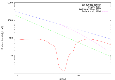
Figure 1: Gas surface densities according to different works. The red curve shows the result of a hydro-dynamical simulation by Morbidelli & Crida (2007), with Jupiter and Saturn in the mutual 2:3 resonance. This is the profile that we assume in this paper, possibly scaled by a factor $f_{d}$. The blue line is from Weidenschilling (1977) and is proportional to $1/r$. The green line is from Hayashi (1981) and is proportional to $1/r^{3/2}$. The magenta curve reports the amount of gas required in Pollack et al. (1996) model of giant planet accretion.

The concept of MMSN was historically introduced assuming that giant planet formation was 100% efficient. In reality, there is growing evidence that much more mass is needed to grow the giant planets, even in the most optimistic scenarios (Thommes et al. 2003). Therefore, in our simulations we multiply the assumed initial surface density profile by a factor $f_{d}$, which will be specified from simulation to simulation. All simulations are run for $5\,$My and for simplicity we assume that the gas density is constant over this simulated timescale. The role of the $5\,$My parameter will be discussed in Sect. 4. In our code, the surface density profile of the gas is used to compute the migration and damping forces acting onto the embryos, namely the so-called “type-I torques”. The analytic formulae that we use are those reported in Cresswell & Nelson (2008); they depend on the local surface density of the disk and on the embryos’ eccentricities and inclinations. Because inward migration can be significantly slower in realistic disks with radiative transfer than in ideal, isothermal disks, we give ourselves the possibility of multiplying the forces acting on the embryo’s semi-major axes by a factor $1/f_{I}$, which will be specified below for each simulation.

However, in Sect. 5, we use a more sophisticated formula for the radial migration torque $\Gamma$, which accounts for the radial gradient of the surface density (Paardekooper et al. 2010; Lyra et al. 2010):

$$\Gamma=\Gamma_{0}(-0.85-\alpha-0.9\beta)\ ,$$ (1)

where $\Gamma_{0}=(M/h)^{2}\Sigma r^{4}\Omega^{2}$, $M$ is the mass of the embryo relative to the Sun, $h$ is the scale-height of the disk normalized by the semimajor axis, $\Sigma$ stands for the local surface density, and $\Omega$ is the orbital frequency. In (1)

$$\alpha=-{{d\log\Sigma}\over{d\log r}}\ ,\quad\beta=-{{d\log T}\over{d\log r}}\ ,$$ (2)

where $T$ is the local temperature of gas.

The radial migration torque in Cresswell & Nelson (2008), at zeroth order in eccentricity and inclination, corresponds to (1) for $\beta=1$ and $\alpha=0$, i.e. it is valid for a flat disk with constant scale height. The inclusion of the $\alpha$-dependence in (1) stops inward migration where $\alpha=-1.75$, that is where there is a steep positive radial gradient of the surface density. With the surface density profile shown in Fig. 1, this happens at $\sim$$10\,$AU. This location acts like a planet trap (Masset et al. 2006): an embryo migrating inwards from the outer disk, if not trapped in a mean motion resonance with Saturn, is ultimately trapped at this location.

In the simulations that mimic turbulent disks (see Sect. 7), we simply apply stochastic torques to the embryos following the recipe extensively described in Ogihara et al. (2007); see Sect. 2.2 of that paper). The only difference is that the total number of Fourier modes in the torque spectrum is not $m=50$, as in Ogihara et al. (2007), but is $m=50/\log 4\times log(r_{\rm out}/r_{\rm in})$ which, given $r_{\rm out}=24\,$AU and $r_{\rm in}=8\,$AU in our case, makes $m=40$. This functional form for $m(r_{\rm out},r_{\rm in})$ is necessary in order to make the results independent of the simulated size of the disk. In fact, if one used a fixed number of Fourier modes, the effect of turbulence would be stronger in a narrow disk than in an extended disk. With our recipe for the number of modes, the stochastic migration of planetesimals observed in the full MRI simulations of Nelson & Gressel (2010) is reproduced with a “turbulent strength” parameter $\gamma$ (see eq. 6 in Ogihara et al. (2007)) equal to $3\times 10^{-3}$.

A final technical note concerns the treatment that we reserve to Jupiter and Saturn. The migration of these two planets is a two-planet Type-II-like process (Masset & Snellgrove 2001; Morbidelli & Crida 2007), and therefore cannot be described with the Type-I torques reported above. As stated in the Introduction, we assume that the disk parameters are such that Jupiter and Saturn do not migrate (see Morbidelli & Crida (2007), for the identification of the required conditions). Consequently, one could think that we should apply no fictitious forces to these planets. However, if we did so, the system would become unstable. In fact, as soon as an embryo is trapped in a resonance with Saturn, it would push Saturn inwards and in turn also Jupiter (because Jupiter and Saturn are locked in resonance). This would also increase the orbital eccentricities of the two major planets. This behavior is obviously artificial, because we do not consider the forces exerted by the gas onto Jupiter and Saturn, which would stabilize these planets against the perturbations from the much smaller embryo. To circumvent this problem, we apply damping forces to Jupiter and Saturn so that $(de/dt)/e=(di/dt)/i=10^{-5}$/y, together with a torque that tends to restore the initial semi-major axes of their orbits in $10^{5}$ years. Tests show that, with this recipe, Jupiter and Saturn are stable under the effect of embryos piling up in resonances and pushing inwards. Moreover the eccentricities of Jupiter and Saturn attain finite but non-zero limit values. However strong scattering events can remove Jupiter and Saturn from their 2:3 resonance (see Sect. 4).

3 Basic dynamical mechanisms in mutual migration of embryos and giant planets

To illustrate the interplay between migration, resonance trapping and mutual scattering, in this section we do simple experiments, where we introduce in the system one embryo at the time. The time-span between the introduction of two successive embryos is not fixed: we let the system relax to a stable configuration before introducing a new embryo in the simulation. Each embryo has initially $3\,$M_⊕.

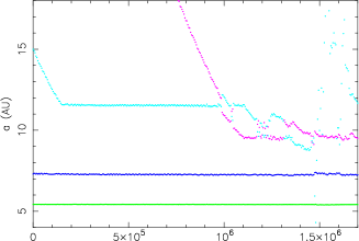
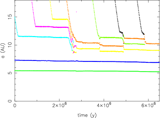
Figure 2: Simulations of the dynamical evolution of embryos in the disk outside of Saturn’s orbit. Top: a case with parameters $f_{d}=f_{I}=1$. Bottom, a case with $f_{d}=f_{I}=2$. The green and blue curves at $\sim$$5.4$ and $\sim$$7.3\,$AU show the semi-major axis evolution of Jupiter and Saturn, respectively. The other curves of various colors illustrate the evolution of the semi-major axes of the embryos. See text for a description of the dynamical evolution and the accretion events.

We start by assuming the nominal values of the parameters ($f_{d}=1$, $f_{I}=1$). The top panel of Fig. 2 shows the evolution. The first embryo is introduced at the beginning of the simulation at $15\,$AU. It migrates inwards (cyan dotted curve) until it is trapped in resonance with Saturn (precisely the 1:2 MMR) at $t\sim 150,000\,$y. Thus, it stops migrating. Resonance trapping converts the force acting onto the semi-major axis into an eccentricity excitation. Thus, the eccentricity of the embryo grows to about 0.07 but then it stops (not shown in the figure). This happens because a balance is reached between the eccentricity excitation from the resonance and the direct damping from the disk. Thus, the three-planet system (Jupiter, Saturn and the embryo) reaches a stable, invariant configuration at about $t=200,000\,$y.

At $t=750,000\,$y we introduce a second embryo in the system, initially at $18\,$AU. This embryo also migrates inward (magenta dotted line). Because of the relatively large eccentricity of the cyan embryo, its outer MMRs are not stable enough to capture the incoming magenta embryo. Thus the latter comes down to $\sim$$12\,$AU and starts to have close encounters with the cyan embryo. The system becomes unstable. The eccentricities and inclinations of the embryos become very large, up to 0.6$-$0.7 and 10 degrees respectively. The cyan embryo has even close encounters with Saturn and Jupiter. It is clear that this phase of violent scattering is not very favorable for embryo-embryo accretion.

We then present another simulation, where we increase the gas surface density by a factor of two ($f_{d}=2$), which has the effect of increasing both the eccentricity/inclination damping and the radial migration by the same factor. However, we also assume $f_{I}=2$, so that the migration rate of the semi-major axis is in fact the same as in the previous simulation. The result of this new simulation is illustrated in the bottom panel of Fig. 2. As one can see, the magenta embryo is now trapped in resonance with the cyan embryo (precisely, the 4:5 MMR). So, it also stops migrating and a stable four-planet configuration is achieved. Given that the only difference with respect to the previous simulation is the eccentricity damping, this illustrates the crucial role of this parameter on the dynamics.

A third embryo (yellow) is introduced at $t=1.6\,$My. It also migrates until it stops, trapped in the 6:7 MMR with the cyan embryo. The fully resonant system is, again, stable.

A fourth embryo is then released at $t=2.3\,$My (orange). Now there are too many embryos to form a stable, resonant system. So, when the orange embryo comes in, resonance locking is broken. All embryos move inward and start to have encounters with each other. Because of the stronger damping from the disk, the eccentricities and inclinations do not become as large as in the previous experiment. Thus, the conditions are more favorable for mutual accretion. In fact, at $t=2.64\,$My the yellow and cyan embryos accrete each other. Arbitrarily, we assume that it is the yellow embryo that survives, with twice its original mass and the cyan embryo disappears. The system of embryos, however, is still too excited to be stable. It stabilizes only after the ejection of the magenta embryo at $t=2.9\,$My. The system is now made of two embryos, the yellow and orange ones, in their mutual 6:7 MMR. The yellow embryo is in the 2:3 MMR with Saturn.

We proceed the experiment by introducing a new embryo (green) which, after a short phase of instability, ends in the 4:5 MMR with the orange embryo and forces the orange and yellow embryos to go to smaller heliocentric distances: the yellow embryo ends in the 5:7 MMR with Saturn. Given the high-order resonances involved, the system is close to an instability.

Thus, when the next embryo (black) is introduced and moves inwards, the system becomes unstable. The new crisis is solved with the yellow embryo accreting the black one. At the end of the instability phase, the yellow embryo is back into the 2:3 MMR with Saturn and the three surviving embryos are in resonance with each other.

The final embryo is introduced at $5.5\,$My (black again). The new embryo generates a new phase of instability during which it first collides with the orange embryo, then the orange embryo accretes also the green one. Therefore, this simulation ends with two embryos, each with a mass of $9\,$M_⊕, in a stable resonant configuration: the yellow embryo is in the 2:3 MMR with Saturn and in the 6:5 MMR with the orange one.

These experiments, as well as other similar ones that we do not present for brevity (with $f_{d}=f_{I}=3,5$ and $f_{d}=1$, $f_{I}=3$), show well the importance of mutual resonances in the evolution of the embryos. For individual masses equal to $3\,$M_⊕, embryos are easily trapped in mutual resonances if $f_{I}\geq 2$. If the embryos are smaller, $f_{I}$ needs to be larger, because the mutual resonant torques are weaker. A system of several embryos, all in resonance with each other, can be stable; if this is the case, mutual accretion is not possible. However, when the embryos are too numerous, resonances cannot continue to hold the embryos on orbits well separated from each other. The system eventually has to become unstable; collisions or ejections then occur. Finally, when the number of embryos is reduced, a new, stable resonant configuration is achieved again. This sequence of events (resonance loading, global dynamical instability, accretion or ejection) can repeat cyclically, as long as mass is added to the system. Eccentricity and inclination damping from the disk also plays a pivotal role in the evolution of the system. If damping is weak, eccentricities and inclinations can become large and scattering dominates over mutual accretion; eventually embryos encounter Jupiter or Saturn and are ejected from the system. If damping is large, the most likely end-state of a dynamical instability is the mutual accretion of embryos, which leads to the growth of massive planets.

Of course, the experiments presented in this section are not realistic, as embryos are introduced one by one. They are just intended to illustrate the basic dynamical mechanisms at play. In the next section, we present more realistic simulations, with all embryos simultaneously present from $t=0$.

4 A first attempt to form Uranus and Neptune

We present a series of simulations with 14 embryos originally distributed in semi-major axis from 10 to $35\,$AU. The initial orbits have low eccentricities ($e\sim 10^{-2}$) and inclinations ($i\sim 10^{-2}\,$rad) relative to the common invariable plane of the system. The initial mass of each embryo is assumed to be $3\,$M_⊕ and the mutual orbital separation among embryos is 5 mutual Hill radii. We run simulations with $f_{d}=1$, 3, and 6, which progressively increase the effects of eccentricity/inclination damping. As well, we divide the speed of Type-I migration, by the factor $f_{I}=1$, 3, or 6. For each of these 9 combinations of $f_{d}$ and $f_{I}$, we perform 10 simulations with embryos having different initial, randomly generated, sets of position and velocity vectors (but which satisfy the above-mentioned distribution properties). Every simulation is run for $5\,$My, a typical lifetime for the disk, during which we keep constant the density of the gas (i.e. the values of $f_{d}$ and $f_{I}$).

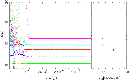
Figure 3: The evolution of the semi major axes of the embryos in simulation No. 7 with $f_{d}=f_{I}=3$. Each color represents a different embryo. The system stabilizes in $\sim 1.2\,$My. The panel on the right shows the final masses of the embryos/cores, as a function of their semi major axes.

Fig. 3 shows evolution of the system for a simulation $f_{d}=f_{I}=3$. The embryos migrate towards Jupiter and Saturn and they have frequent encounters with each other, which makes the evolution very chaotic. Several of them have also close encounters with Jupiter and Saturn and consequently are scattered onto distant elliptic orbits or into the inner Solar System. Through these scattering events and mutual collisions, the number of embryos beyond Saturn eventually decreases to 3 in $1.5\,$My and the surviving bodies find a stable resonant configuration. The most massive object has grown to $9\,$M_⊕ whereas the two others have preserved their initial mass ($3\,$M_⊕). The three embryos that have been scattered into the inner Solar System eventually accrete with each other forming a 9 Earth-mass object. Because the system remains “frozen”, once a resonant stability is achieved, the lifetime of the gas-disk would not influence significantly the results. In the case illustrated in this figure any lifetime longer than $1.5\,$My would produce the same final system. Instead, if the lifetime had been shorter than $1.5\,$My the system would not have reached the final state, leaving many embryos on eccentric and chaotic orbits.

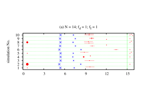
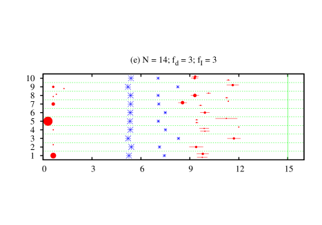
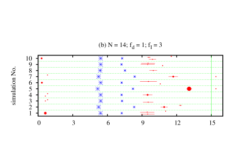
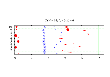
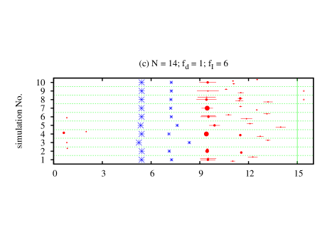
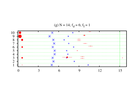
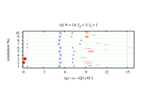
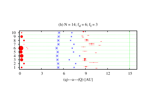
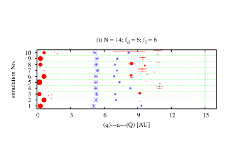
Figure 4: The end-states (in $5\,$Myr) of the simulations starting with 14 embryos, each with $3\,$M_⊕. The simulations are separated by horizontal dashed green lines. The surviving embryos/cores are shown with filled red dot, whose size is proportional to the objects mass. The scale is shown on the bottom panel. The red horizontal bar shows the perihelion-aphelion excursion of these objects on their eccentric orbits. The objects beyond $15\,$AU are plotted for simplicity at $15.5\,$AU, beyond the vertical solid green line. Jupiter and Saturn are shown as blue asterisks. The label on top of each panel reports the number $N$ of embryos and the values of $f_{I}$ and $f_{d}$ adopted in the simulations.

Fig. 4 shows the end-states of the simulations for all combinations of $f_{I}=1$, 3, 6 and $f_{d}=1$, 3, 6. The number of bodies surviving beyond Saturn changes from 1 to 3 for one simulation to another. Similarly, the mass of the body in the inner Solar System changes from 3 to $27\,$M_⊕. Notice that Saturn is not always in the same position relative to Jupiter, despite of the forces that we applied to keep these planets in the mutual 2:3 resonance. In fact, in some cases Saturn moves out of the 2:3 resonance while scattering an embryo inwards; then the forces drive it back towards Jupiter but Saturn is caught in a resonance other than 2:3 (mostly 1:2 or 1:3). This evolution depends on the magnitude of the migration forces that we impose. We have checked that, if we increase the strength of the migration forces by an order of magnitude, Saturn goes back to 2:3 resonance in all of the simulations. Notice that the hydrodynamical simulations (Pierens & Nelson 2008) show that in the MMSN disk Saturn always reaches 2:3 resonance with Jupiter.

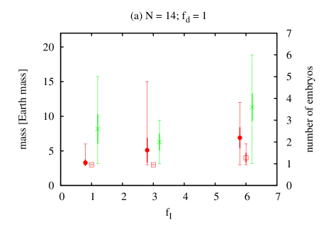
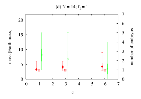
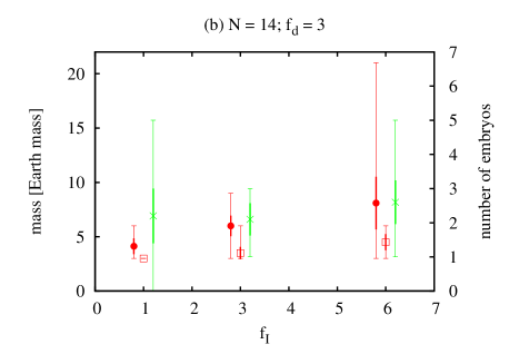
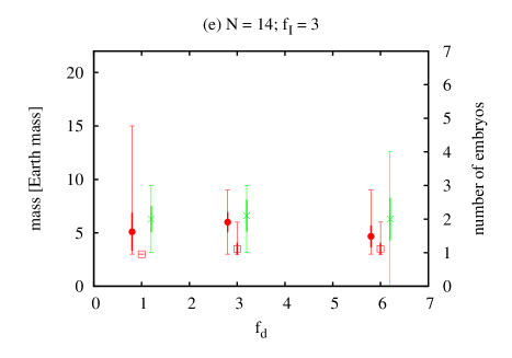
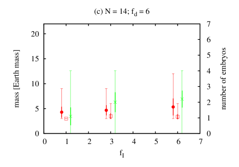
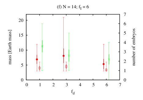
Figure 5: Statistical analysis of the results of the simulations starting from 14 embryos. The $x$-axis of left plots reports the value of $f_{I}$ at fixed $f_{d}$, given at the title of each plot. Similarly, the $x$-axis of right plots reports the value of $f_{d}$ at fixed $f_{I}$. The dot, slightly displaced to the left, is the mean mass of the largest core surviving beyond Saturn, computed over the corresponding 10 simulations. The thick vertical bar is the rms deviation of this quantity. The thin bar shows the excursion of the same quantity from minimum to maximum. The square, in the middle, and related bars are the same, but for the second largest core. The mass scale is reported on the left of the diagram. The cross, slightly displaced to the right, reports the mean number of embryos/cores surviving beyond Saturn, to be read against the scale on the right hand side. Again, the thick bar is for the rms deviation and the thin bar for the minimum-maximum quantity.

We now discuss the statistical dependence of the results on the values of $f_{d}$ and $f_{I}$. Fig. 5 shows the number of bodies surviving in the system as well as the masses of the first and second largest bodies beyond Saturn, as a function of these parameters.

It is clear from the figure, that there are no statistically significant trends of the considered quantities with respect to the investigated disk parameters. There is however a significant trend that is apparent from the panels in the Fig. 4: the mass of the body formed in the inner Solar System increases on average with $f_{d}$ and $f_{I}$. If these parameters are small several embryos are ejected from the system or can be found on distant orbit; instead if $f_{d}$ and $f_{I}$ are larger, no bodies are ejected and most of the objects scattered by Jupiter and Saturn end up in the inner Solar System. Notice that the injection of embryos inside the orbit of Jupiter (which happens in most simulations) is probably inconsistent with the current structure of the Solar System, but might explain the structure of some extra-solar planetary systems, particularly those with a hot Neptune and a more distant giant planet like HD 215497. Similarly, the ejection of embryos onto distant, long-period orbits, might find one day an analog in the extra-solar planet catalogs.

Overall our results concerning the formation of the cores of Uranus and Neptune are disappointing. The best cases are simulation No. 4 with $(f_{d},\leavevmode\nobreak\ f_{I})=(1,\leavevmode\nobreak\ 6)$ and No. 8 with $(f_{d},\leavevmode\nobreak\ f_{I})=(6,\leavevmode\nobreak\ 6)$, both producing beyond Saturn two cores of 12 and $6\,$M_⊕, together with one leftover embryo. Thus, in general, although the mass of the first core is close to the mass of Uranus, the mass of the second biggest core is never large enough to correspond to Neptune.

One could think that our inability to produce two objects as massive as Uranus and Neptune is due to an insufficient total mass in embryos in the initial disk beyond Saturn. To investigate if this is true, we performed another series of simulations with more embryos and, therefore, a higher initial total mass. Specifically, we consider 28 embryos distributed in the same range of heliocentric distances, from 10 to $35\,$AU. The initial mass of each embryo is assumed to be $3\,$M_⊕, again. With this set-up, the orbital separation between embryos is on average smaller than 5 mutual Hill radii. So, the embryos are on orbits which are closer to each other than predicted by the theory of runaway/oligarchic growth (Kokubo & Ida 1998). We nevertheless assume such initial configurations in order to explore how the results change by doubling the total initial mass.

In the simulations with 28 embryos, the masses of the cores surviving beyond Saturn do not improve significantly, relative to the 14-embryos cases. (The final masses and orbital characteristics of the surviving objects in the 28-embryos simulations can be seen in Fig. A1.) The main effect of the doubled initial mass is in the mass of the cores formed in the inner Solar System, the most massive of which reaches $57\,$M_⊕ (simulation No. 8 for $(f_{d},\leavevmode\nobreak\ f_{I})=(6,\leavevmode\nobreak\ 3)$).

Statistically, no significant trend can be seen. (The statistical dependence for all combinations of $f_{d}$ and $f_{I}$ is shown in Fig. A2.) There are no significant differences from the results obtained with half the initial mass. The mass in excess in the new runs has ended up in the large cores in the inner Solar System, but it does not contribute to form bigger cores beyond Saturn. The most massive core surviving beyond Saturn has $24\,$M_⊕ (simulation No. 7 for $(f_{d},\leavevmode\nobreak\ f_{I})=(3,\leavevmode\nobreak\ 6)$) but there is no second core. The best system is that achieved in simulation No. 1 for $(f_{d},\leavevmode\nobreak\ f_{I})=(1,\leavevmode\nobreak\ 6)$, with cores of 15 and $9\,$M_⊕ beyond Saturn (together with three leftover embryos). These best case results are better than those achieved starting from 14 embryos but still they do not successfully reproduce the real case of Uranus and Neptune.

5 A “planet trap” at the edge of Saturn’s gap

In the previous section we have seen that a large fraction of the initial embryo population is lost due to migration into the Jupiter-Saturn region. Most of the embryos that come too close to the giant planets are eliminated because of collisions with Jupiter and Saturn, ejection onto hyperbolic orbits or injection into the inner Solar System.

This result may be due to the fact that the migration torque that we implemented (from Cresswell & Nelson (2008) see Sect. 2), does not take into account the so-called coorbital corotation torque (Masset 2001). This torque would stop inward-migrating embryos at a “planet trap” just inward of the outer edge of the gap opened in the disk of gas by Jupiter and Saturn (Masset et al. 2006). The planet trap would prevent the embryos from coming too close to the giant planets. To test what effects this would have on planetary accretion and evolution, we have done simulations implementing a new formula from Paardekooper et al. (2010), which accounts for the co-orbital corotation torque, as explained in Sect. 2.

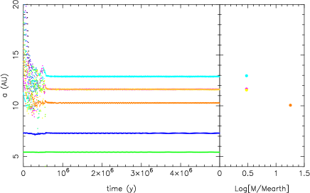
Figure 6: The same as Fig. 3 but for No. 3 with $f_{d}=3$, $f_{I}=1$ and accounting for the planet trap.

To reduce parameter-space we fixed $f_{I}=1$. This is legitimate, because in principle, there is no need to reduce Type-I migration speed as it automatically decreases to zero approaching $\sim$$10\,$AU. We did three series of 10 simulations for $f_{d}=1$, 3, and 6. All started with a system of 10 embryos of $3\,$M_⊕, originally distributed from 11 to $34\,$AU, with a mutual orbital separation of 7 mutual Hill radii. (The end-states are illustrated in Fig. A3.) Fig. 6 gives an example of evolution taken from simulation No. 3 with $f_{d}=3$. It is instructive to compare this figure with Fig. 3 above. In this case we see much fewer embryos coming into the Jupiter-Saturn region and suffering scattering events. This is precisely the effect of the planet trap. As a consequence, 90 percent of the initial embryos mass is retained in the system beyond Saturn, whereas only 38 percent of the mass was retained in the case of Fig. 3. Notice also that the accretion process lasts for a shorter time ($0.6\,$My against $1.2\,$My, respectively), because the system of embryos/cores remains less dynamically excited.

Nevertheless, we see from Fig. 6 that only one core grows massive ($18\,$M_⊕) and the rest of the mass ($9\,$M_⊕ in total) is splitting in three leftover embryos, that are on stable orbits in resonance with the massive core and with each other. Notice, the presence of two embryos in co-orbital configuration, at $\sim$12 AU. This result is typical as can be checked in Fig. A3. This is very different from the case of the Solar System, with two major planets of comparable masses beyond Saturn (Uranus and Neptune) and no leftover embryos.

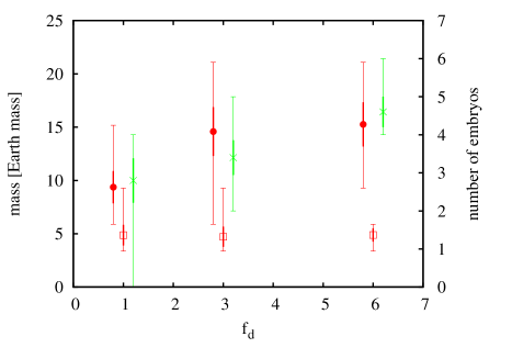
Figure 7: The same as Fig. 5 but for the simulations with the planet trap.

Fig. 7 shows the statistical analysis of our results as a function of the parameter $f_{d}$. We see a trend, although only marginally significant: the mass of the largest core and the number of bodies surviving beyond Saturn increases with $f_{d}$. However, the mass of the second largest object is remarkably independent of $f_{d}$ and it is small in all cases. We interpret this result as follows: A larger value of $f_{d}$ increases the eccentricity damping on the embryos. With smaller eccentricities, the embryos have a larger gravitational focusing factor (Greenzweig & Lissauer 1992) and therefore they can accrete each other more easily. However, because embryos tend to cluster at the location of the planet trap, basically only the innermost embryo, i.e. the one located the nearest to the trap, gets the benefit of the situation.

Overall, these experiments show that the planet trap is very effective in reducing the loss of mass during the embryo’s evolution. Still, the final results are not in good agreement with the structure of the Solar System. In fact, only one major core grows and the rest of the mass remains stranded in too many embryos in stable resonant configuration. Consequently, despite initially we have a total mass comparable to the combined mass of Uranus and Neptune, at the end only one massive planet is formed.

To test how these results would change with the total mass initially available in embryos, we ran a series of 10 additional simulations starting with 15 embryos of $3\,$M_⊕. The orbits of the embryos were initially separated by 5 mutual Hill radii and were distributed from 10 to $35\,$AU. For simplicity, we fixed $f_{d}=3$. No statistically significant trend with the initial total mass in the system appears (the end-states are reported in Fig. A3) , so that the problems discussed above (too small mass of the second core and too many resonant leftovers) remain. This implies that the additional mass is typically lost. Nevertheless, we have got one simulation whose result is about perfect relative to the Solar System structure, with only two cores surviving beyond Saturn, each with a mass of $15\,$M_⊕ (see Fig. 8).

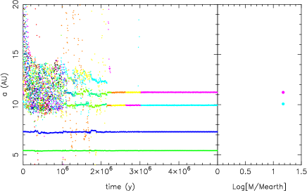
Figure 8: The same as Fig. 3 but for the only simulation (No. 2) that successfully produces Uranus and Neptune.

6 The initial mass of the embryos

All the simulations presented up to this point in the paper started from a system of embryos of individual mass equal to $3\,$M_⊕. In this section we study the influence of the individual mass of the embryos on the final results. Following the structure of the paper, we first present a series of simulations which do not account for the presence of a planet trap at the edge of Jupiter/Saturn’s gap, then we focus on the impact of the planet trap.

6.1 Without a planet trap

In this new series of simulations, we reduced the initial mass of embryos from 3 to $1.5\,$M_⊕. However, we increased the number of embryos from 14 to 28, thus preserving the total mass of the system used in the first part of Sect. 4. The embryos are initially located in the 10$-$35-AU interval with mutual orbital separations of 3.8 mutual Hill radii.

As in Sect. 4, we performed 10 simulations for each combination of $f_{I}=1$, 3, 6 and $f_{d}=1$, 3, 6. We find much less growth than in the equivalent simulations of Sect. 4, starting with $3\,$M_⊕. This is due to the migration and damping forces are linear in the mass of the embryos and therefore are weaker in this case. Thus, under their mutual encounters the embryos become more dynamically excited and their collision probability decreases dramatically. Most of the simulations with $f_{d}=1$ and $f_{I}=3$, 6 did not reach a stable final configuration at $5\,$My and when many embryos are still on highly eccentric and mutually crossing orbits. We find the most significant growth in the runs with $f_{d}=3$ and $f_{I}=6$, but only one major core is produced, with a mean mass of $8\,$M_⊕. The runs with $f_{d}=6$ and $f_{I}=6$ transfer most of the mass in the inner Solar System. (The end-states of these simulations are summarized in the Fig. A4.)

The statistical analysis of our results (Fig. A5) reveals no correlation of the results with $f_{d}$ for any value of $f_{I}$. However, we find some correlation between the mass of the largest core and the value of $f_{I}$ for each value of $f_{d}$. Remember that in absence of a planet trap, embryos are driven by migration to encounter the giant planets, unless they are trapped in resonance with Saturn. The larger is $f_{I}$, the slower is migration and therefore the easier is for embryos to be stopped in resonance and (possibly) accrete with each other. This may explain the observed correlation.

6.2 With a planet trap

We did a series of 10 simulations, starting from 30 embryos, each of $1\,$M_⊕, thus preserving the total mass of the system used in the first part of Sect. 5. They are initially distributed from 9 to $35\,$AU, with a mutual orbital separation of 4.5 mutual Hill radii. We fixed $f_{I}=1$ and $f_{d}=3$. The end-states are reported in Fig. A3.

The results are significantly different from those of the runs starting from more massive individual embryos, reported in Sect. 5. On average, the mass of the largest core beyond Saturn drops by a factor of 2 and that of the second largest core drops by a factor of 1.5. These drops are statistically significant. The mean number of surviving cores/embryos is 4, with simulations producing up to 7 objects. Therefore the results are very far from the structure of the current Solar System. More mass is lost in these simulations than in the corresponding simulations starting from more massive embryos. As said above, this is probably because the forces damping the eccentricities and inclinations of the embryos are weaker.

7 The effect of turbulence in the disk

The problems that we experienced in the previous sections due to embryos and cores being protected by resonances from mutual collisions suggests that some level of turbulence in the disk might promote accretion. In fact, turbulence provides stochastic torques onto the bodies, inducing a random walk of their semi-major axes (Nelson & Gressel 2010). If these torques are strong enough, the bodies may be dislodged from mutual resonances, which in turn would allow them to have mutual close encounters and collisions.

The problem is that it is not known a priori how strong turbulence should be in the region of the disk where giant planets form. The strength of MRI turbulence depends on the level of ionization of the disk (Fleming et al. 2000), and it is possible that in the massive regions of the disk where giant planets form the ionization of the gas is very low because the radiation from the star(s) cannot penetrate down to the midplane (Gammie 1996). Several formation models, therefore, argue that the planets form in a “dead zone” where, in absence of ionization, there is no turbulence driven by the magneto-rotational instability. This justifies the assumption that we made up to this point in the paper that the disk is laminar.

For the sake of completeness, though, we test in this section how the results change if strong or weak turbulence is assumed in the disk. The experiments are conducted in the framework of the planet trap case, with 10 embryos of $3\,$M_⊕ (see Sect. 5). As in previous section 6.1 we assume $f_{I}=1$ and $f_{d}=3$. We performed three sets of 10 simulations with three different values of the turbulent strength $\gamma$. We used $\gamma=3\times 10^{-4}$, $1\times 10^{-3}$ and $3\times 10^{-3}$. The latter correspond to strong turbulence without dead-zone (Baruteau & Lin 2010). The end-states are, again, reported in Fig. A3.

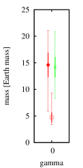
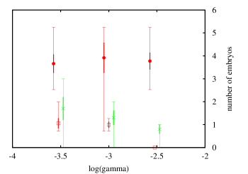
Figure 9: The same as Fig. 5 but for the series of simulations with different turbulence strength $\gamma$. The series for $\gamma=0$ (no-turbulence) is that presented in Sect. 5.

Fig. 9 reports a statistical analysis of our results. There is a clear correlation, with the number of objects surviving beyond Saturn decreasing with increasing strength of the turbulence, as expected. The runs with $\gamma=3\times 10^{-3}$ typically leave only one object beyond Saturn. The mass of the second largest core also decreases with increasing turbulence. Instead we do not see any statistical correlation between the mass of the largest core and the turbulence strength. This is a surprise, because we expected that, with fewer embryos stranded in resonant isolation, the largest core would have grown more massive. In reality, though, it seems that more mass is lost as the turbulence increases so that the largest core does not benefit from the situation. The reason for this is clearly that resonant configurations are not stable if turbulence is too strong. Fig. 10 gives an illustration of this, showing the evolution of the system in simulation No. 6 with $\gamma=3\times 10^{-3}$. We can see a stochastic behavior of the semi-major axis of the cores, that eventually forces the last two cores to collide with each other. The surviving core in this simulation has the mass of $24\,$M_⊕, which is the largest among all objects produced in our turbulence simulations. Typically, more objects interact with Jupiter and Saturn and are eventually lost.

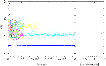
Figure 10: The same as Fig. 3 but for a simulation with strong turbulence (No. 6 with $\gamma=3\times 10^{-3}$).

We conclude from these tests that turbulence may be helpful to break the isolation of planets and to avoid the formation of a too crowded planetary system beyond Jupiter and Saturn. However, the formation of two massive cores, with no left-over embryos seems to be still a distant goal, as typically only one core is produced.

8 Conclusions and Discussions

The formation of Uranus and Neptune by runaway/oligarchic growth from a disk of planetesimals is very difficult. The accretion rate is not large enough; moreover the accretion stalls when the major bodies achieve a few Earth masses (Safronov 1969; Levison & Stewart 2001; Levison & Morbidelli 2007).

In this paper, we have explored a mechanism for the formation of Uranus and Neptune that is different from those explored before. We assume that runaway/oligarchic growth from a planetesimal disk generated a system of embryos of 1$-$3 Earth masses, but not larger, in agreement with the results of Levison et al. (2010). Then, we follow the dynamical evolution of such a system of embryos, accounting for their mutual interactions, their interaction with a disk of gas and the presence of fully formed Jupiter and Saturn on resonant, non-migrating orbits. Because of computation speed, we do not perform the simulations with an hydro-dynamical code. Instead, we use an N-body code, and we apply fictitious forces to the embryos that mimic the orbital damping and migration torques that the disk exerts on the embryos. We use two prescriptions for the migration torque: one that ignores the co-orbital corotation torque and one that takes it into account. With the second prescription a “planet trap” (Masset et al. 2006) appears at about $10\,$AU, just inward of the outer edge of the gap opened by Jupiter and Saturn in the disk of gas.

Our results show that the idea works in principle. In many runs, particularly those accounting for a disk a few times more massive than the MMSN and those accounting for the presence of the planet trap, there is significant mass growth. In these cases, the major core beyond Saturn exceeds 10 Earth masses. These results highlight the importance of the planet trap and of the damping effect that the gas-disk has on the orbital eccentricities and inclinations of planetary embryos.

Our simulations typically do not successfully reproduce the structure of the outer Solar System. In the wide range of the end-states due to the stochasticity of the accretion process, only one simulation is successful, with two cores of $15\,$M_⊕ produced and surviving beyond Saturn and no rogue embryos. In general, our results point to at least two major problems. The first is that there is typically a large difference in mass between the first and the second most massive cores, particularly in the simulations showing the most spectacular mass growth. This contrasts with Uranus and Neptune having comparable masses. The second problem appears mostly if we account for the planet trap, so that more material is kept beyond the orbit of Saturn. The problem is that the final planetary system typically has many more than two embryos/cores. Several original embryos, or partially grown cores, survive at the end on stable, resonant orbits. In several cases bodies are found in coorbital resonance with each other. This is in striking contrast with the outer Solar System, where there are no intermediate-mass planets accompanying Uranus and Neptune. It might be possible that these additional planets have been removed during a late dynamical instability of the planetary system, but the likelihood of this process remains to be proven.

Accounting for some turbulence in the disk alleviates this last problem. However, when turbulence is strong enough to prevent the survival in resonance of many bodies, the typical result is the production of only one core.

In addition to the problems mentioned above, there is another intriguing aspect suggested by the results of our model. We have seen that, in order to have substantial accretion among the embryos, it is necessary that the parameter $f_{d}$ is large, namely that the surface density of the gas is several time higher than that of the MMSN. However this contrasts with the common idea that Uranus and Neptune formed in a gas-starving disk, which is suggested by the small amount of hydrogen and helium contained in the atmospheres of these planets compared to those of Jupiter and Saturn. How to solve this conundrum is not clear to us.

In summary, our work does not bring solutions to the problem of the origin of Uranus and Neptune. However, it has the merit to point out non-trivial problems that cannot be ignored and have to be addressed in future work.

Appendix A: additional figures

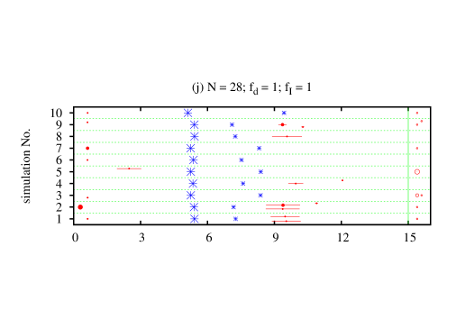
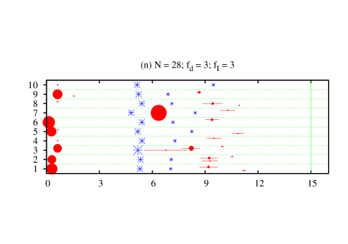
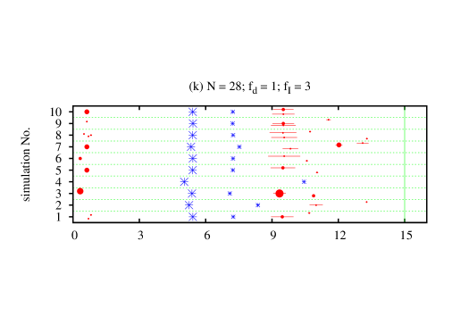
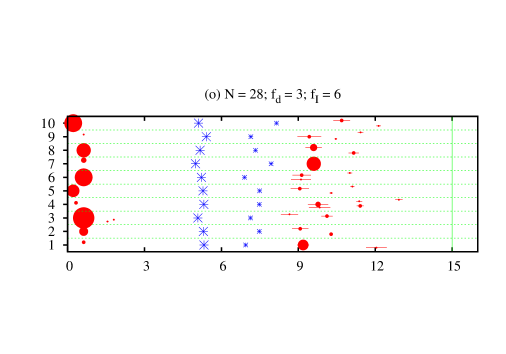
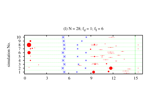
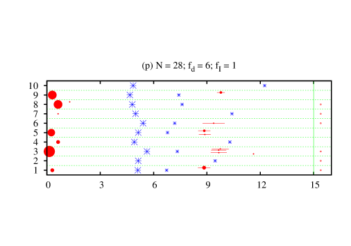
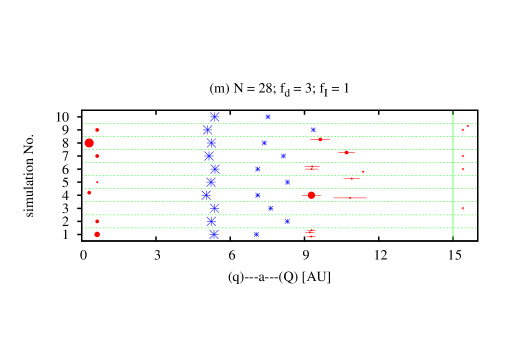
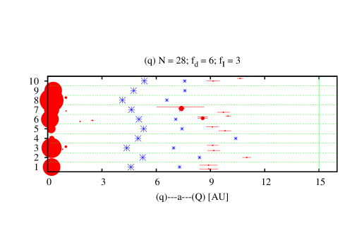
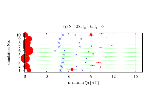
Fig. A 1: The end-states (in $5\,$Myr) of the simulations starting with 28 embryos, each with $3\,$M_⊕. The simulations are separated by horizontal dashed green lines. The surviving embryos/cores are shown with filled red dot, whose size is proportional to the objects mass. The scale is shown on the bottom panel. The red horizontal bar shows the perihelion-aphelion excursion of these objects on their eccentric orbits. The objects beyond $15\,$AU are plotted for simplicity at $15.5\,$AU, beyond the vertical solid green line. Jupiter and Saturn are shown as blue asterisks. The label on top of each panel reports the number $N$ of embryos and the values of $f_{I}$ and $f_{d}$ adopted in the simulations. (For the discussion - see Sect. 4).

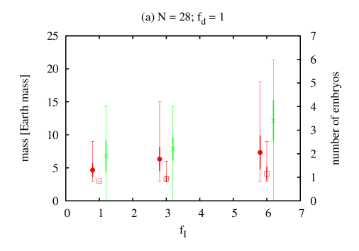
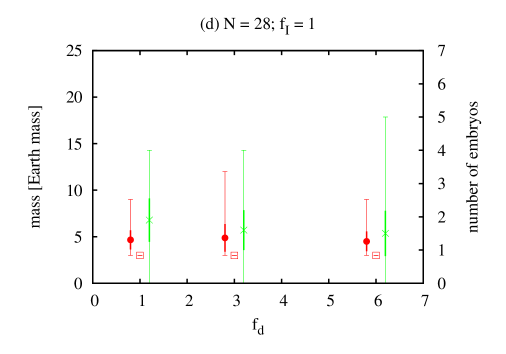
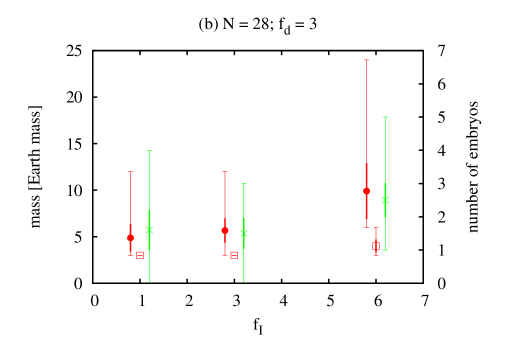
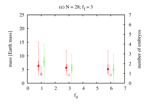
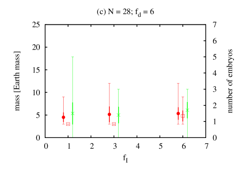
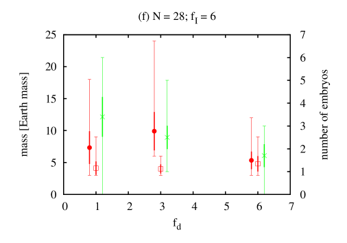
Fig. A 2: Statistical analysis of the results of the simulations starting from 28 embryos, each with $3\,$M_⊕. The $x$-axis of left plots reports the value of $f_{I}$ at fixed $f_{d}$, given at the title of each plot. Similarly, the $x$-axis of right plots reports the value of $f_{d}$ at fixed $f_{I}$. The dot, slightly displaced to the left, is the mean mass of the largest core surviving beyond Saturn, computed over the corresponding 10 simulations. The thick vertical bar is the rms deviation of this quantity. The thin bar shows the excursion of the same quantity from minimum to maximum. The square, in the middle, and related bars are the same, but for the second largest core. The mass scale is reported on the left of the diagram. The cross, slightly displaced to the right, reports the mean number of embryos/cores surviving beyond Saturn, to be read against the scale on the right hand side. Again, the thick bar is for the rms deviation and the thin bar for the minimum-maximum quantity. (For the discussion - see Sect. 4).

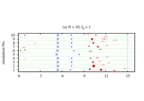
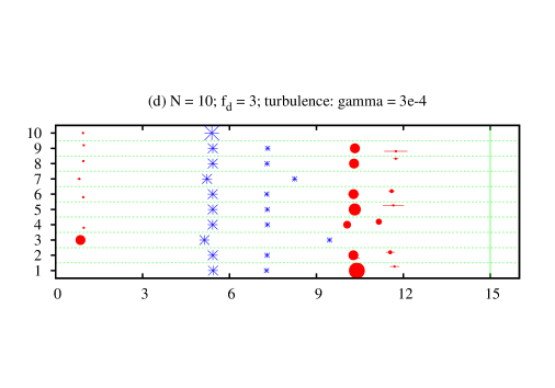
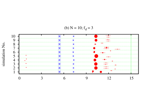
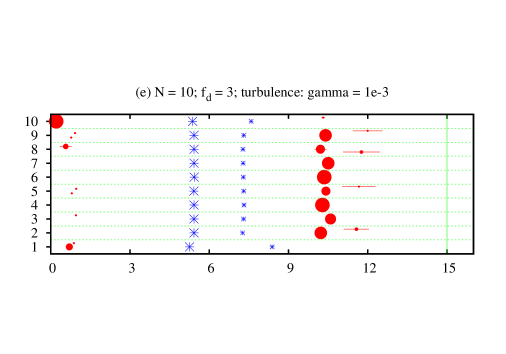
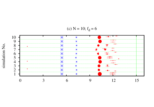
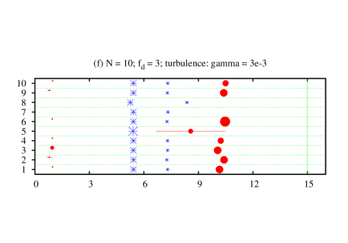
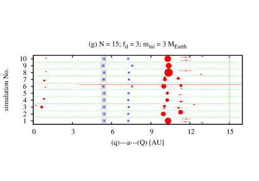
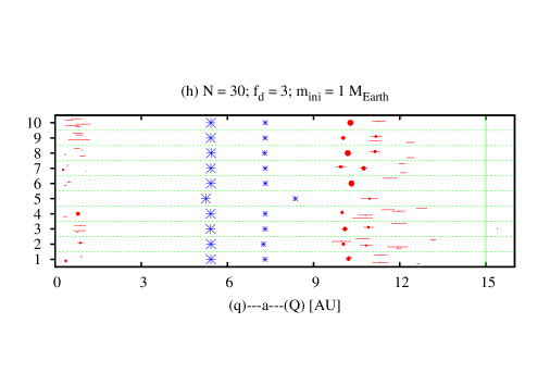
Fig. A 3: The same as Fig. A1 but for the simulations in which the planet trap was considered. The plots (a,b,c) show the end-states starting with initial embryo-mass of $3\,$M_⊕ when the turbulence is not taken into account, plots (d,e,f) are related to the cases with the turbulence characterized by $\gamma=3\times 10^{-4}$, $1\times 10^{-3}$, and $3\times 10^{-3}$, respectively. At the start, 10 embryos are assumed in these simulations. Plot (g) shows the end-states of simulations starting with a higher total mass (15 embryos of $3\,$M_⊕) and plot (h) does this for a larger number of initally less massive embryos (30 embryos of $1\,$M_⊕). (For the discussion - see Sect. 5).

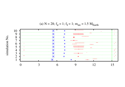
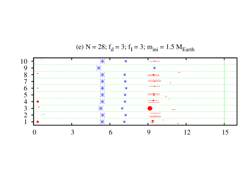
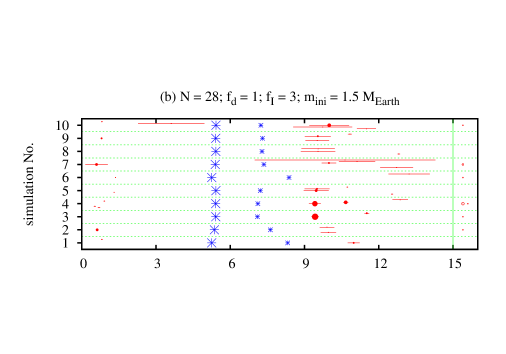
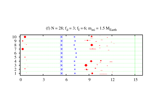
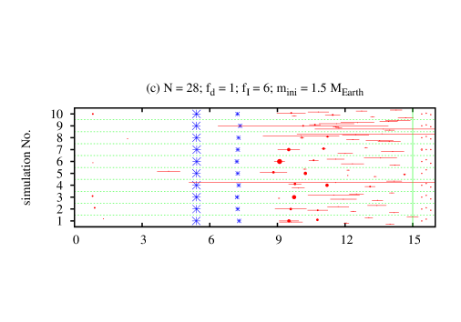
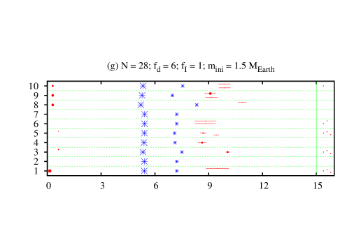
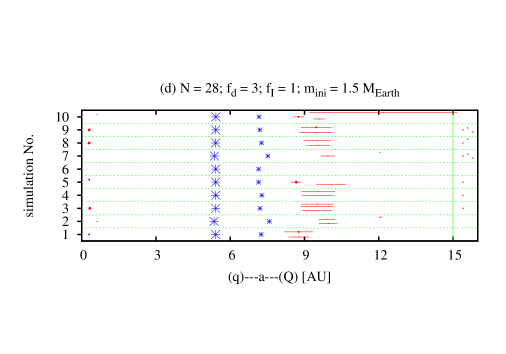
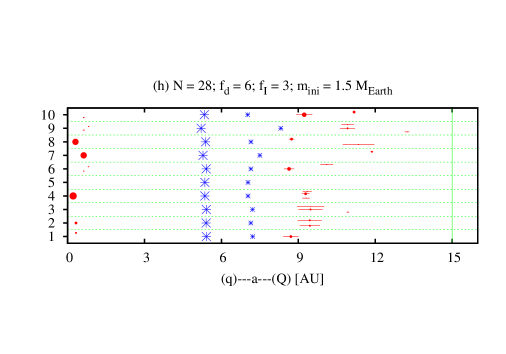
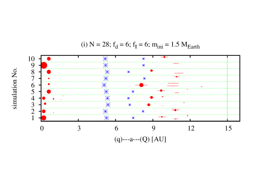
Fig. A 4: The same as Fig. A3 but with the initial mass of each embryo of $1.5\,$M_⊕. (For the discussion - see Sect. 6.1).

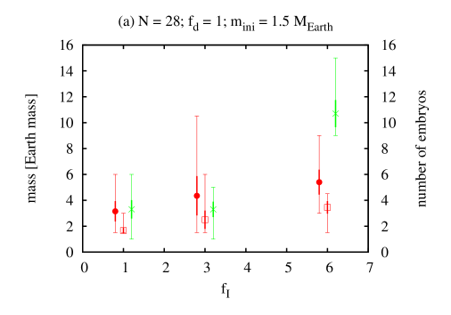
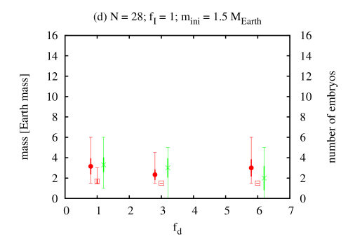
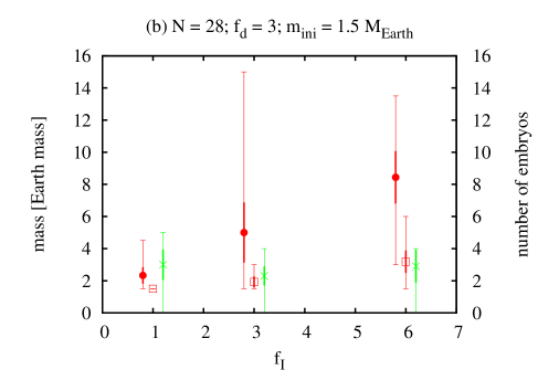
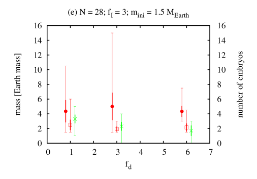
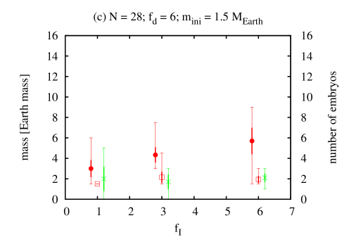
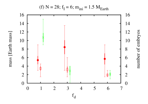
Fig. A 5: The same as Fig. A2 but with the initial mass of each embryo of $1.5\,$M_⊕. (For the discussion - see Sect. 6.1).