Scaling Behavior of Convolutional LDPC Ensembles over the BEC

Abstract

We study the scaling behavior of coupled sparse graph codes over the binary erasure channel. In particular, let $2L+1$ be the length of the coupled chain, let $M$ be the number of variables in each of the $2L+1$ local copies, let $\ell$ be the number of iterations, let $P_{\text{b}}$ denote the bit error probability, and let $\epsilon$ denote the channel parameter. We are interested in how these quantities scale when we let the blocklength $(2L+1)M$ tend to infinity. Based on empirical evidence we show that the threshold saturation phenomenon is rather stable with respect to the scaling of the various parameters and we formulate some general rules of thumb which can serve as a guide for the design of coding systems based on coupled graphs.

I Introduction

Spatially coupled codes [Kudekar10] provide an entirely new way of approaching capacity. The basic phenomena can be phrased as follows: an ensemble constructed by coupling a chain of $(2L+1)$ regular $(l,r)$ low-density parity-check (LDPC) ensembles, together with appropriate boundary conditions of the chain, exhibits a belief propagation (BP) threshold close to the maximum-a-posteriori (MAP) threshold of the regular $(l,r)$ ensemble. This phenomenon is known as threshold saturation and it has been proved rigorously for the binary erasure channel (BEC) in [Kudekar10]. It has also been observed empirically for a variety of other channels and other graphical models in [Tanner04, Lentmaier10, Kudekar10-2]. Low-density parity-check convolutional (LDPCC) ensembles, first introduced in [FelstromZ99], are the best known example of spatially coupled codes. In [Lentmaier09], the authors reformulate LDPCC ensembles in terms of protographs. The BP threshold for these codes is computed using density evolution (DE) in [Lentmaier10, Kudekar10] and it is conjectured that they achieve capacity universally across the set of binary-input memoryless output-symmetric channels [Kudekar10].

It is probably fair to state that by now the asymptotic performance of spatially coupled LDPC codes is well understood. However, much less is known about their scaling behavior [Kudekar10]. For instance, the DE analysis of LDPCC codes typically assumes that $L$ is kept fixed while $M$ tends to infinity. But, does the threshold saturation phenomena happen even if $L$ grows as a function of $M$? In this work, we analyze the finite-length performance of LDPCC codes and we study how it scales with the coupling dimensions $M$ and $L$. Our empirical observations indicate that the threshold saturation phenomenon happens even when $L$ grows considerably faster than $M$, which indicates that the threshold saturation phenomenon is very robust. From our simulation results we synthesize some general design rules for these codes. In particular, if the code-length is bounded, how should we chose $L$ and $M$ to have the best performance? And how does this choice affect the decoder complexity (in terms of average number of iterations)? These questions, among others, are of significantly practical importance.

The study of the finite-length behavior of LDPCC codes is augmented by analyzing their error floor [Urbanke08-2]. In [Kudekar10, Lentmaier10-2], the authors prove that the minimum distance of LDPCC codes is a fraction of $M$. These studies concern “large” weight codewords. We investigate the occurrence of constant-sized codewords/stopping sets, and in particular their scaling. We prove that the fraction of codes with no error floor is roughly equal to $\exp(-cL/M^{l-2})$, where $c$ only depends on the rate of the code. Hence, for sufficiently small ratios $L/M^{l-2}$, it is very easy to expurgate the ensemble and to find codes with linear minimum distance.

II Convolutional-like LDPC ensembles. Basic design parameters

We define the LDPCC ensembles using protographs [Lentmaier09]. We start from a collection of $(2L+1)$ regular $(l,r=kl)$ LDPC protographs with $k\in\mathbb{N}$ [Thorpe03] and so that $l$ is odd, as shown in Fig. 1 for $(l,r)=(3,6)$ and $L=9$. The regular $(l,r=kl)$ code is referred to as the underlying code. The associated protograph has $k$ variable nodes of degree $l$ so that, if $M$ is the total number of variables per protograph, each variable node of the protograph represents $M/k$ variables in total. For instance, in Fig. 1, each variable node of the protograph represents $M/2$ variables. In the following, we say that the LDPCC graph has $(2L+1)$ sections, one per protograph in Fig. 1.

Let us now define the coupled protograph. This graph is constructed by spatially coupling the protographs in Fig. 1: each variable node is connected to its $\hat{l}$ check node neighbors on the left and to its $\hat{l}$ check node neighbors on the right, where $\hat{l}=(l-1)/2$ [Kudekar10]. The coupled protograph is terminated by adding $\hat{l}$ extra check nodes on each side. This process is illustrated in Fig. 2 for the case $(l,r,L)=(3,6,9)$. In the termination procedure described, the check nodes of lower degree on both sides provide better protection for the connected variables. However, there is a price to be payed for this extra protection – the rate is reduced with respect to the rate of the underlying code. The ensemble has $n=M(2L+1)$ variable nodes and $(2(L+\hat{l})+1)M/k$ check nodes and the design rate is:

$$R(l,r=kl,L)=\frac{k-1}{k}-\frac{2\hat{l}}{k(2L+1)},$$ (1)

where the first term is the rate of the underlying code [Kudekar10]. To generate a sample of the LDPCC ensemble we now “lift” the coupled protograph in the same manner as this is done for regular ensembles [Thorpe03]: we make $(M/k)$ copies of the coupled protograph and we connect them by picking for each “edge bundle” a random permutation. In the following we refer to the ensemble as the $(l,r,L,M)$ (convolutional) ensemble.

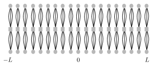
Figure 1: A chain of $(2L+1)$ regular (3,6) non-interacting protographs for $L=9$.

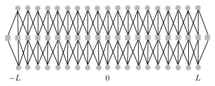
Figure 2: Coupled protograph created from a chain of $(2L+1)$ regular (3,6) protographs for $L=9$.

II-A Asymptotic analysis of the LDPCC ensemble

The performance of spatially-coupled ensembles under BP decoding as $M$ goes to infinity is analyzed in [Lentmaier10, Kudekar10] using density evolution (DE) [Urbanke08-2]. This allows to compute the BP threshold, which defines the limit of the decodable region. Let us denote the threshold for the BEC by $\epsilon^{\text{BP}}(l,r,L)$. We have

$$\lim_{\ell\rightarrow\infty}\lim_{M\rightarrow\infty}P_{b}^{\ell}(\epsilon,l,r,L,M)=0,\;\epsilon<\epsilon^{\text{BP}}(l,r,L),$$ (2)

where $P_{b}^{\ell}(\epsilon,l,r,L,M)$ is the ensemble average bit error probability after $\ell$ decoding rounds:

$$P_{b}^{\ell}(\epsilon,l,r,L,M)=\mathbb{E}_{\mathcal{C}\in(l,r,L,M)}[P_{b}^{\ell}(\epsilon,\mathcal{C})].$$ (3)

Similarly, $P_{B}^{\ell}(\epsilon,l,r,L,M)$ denotes the ensemble average block error probability. One of the key results of the asymptotic analysis of coupled codes is that $\epsilon^{\text{BP}}(l,r,L)$ is “very close” to $\epsilon^{\text{MAP}}(l,r)$, the MAP threshold of the underlying regular ensemble [Lentmaier10].

II-B Finite-length scaling LDPCC codes

Finite-length scaling investigates the relationship between the performance, the code parameters, and the decoding complexity. Any practical design of a LDPCC code starts from a set of constraints on the code rate in (1), the code length, and the number of decoding iterations with the goal of finding the best choice of parameters. To first order, one might wonder for which scaling of $L$ with respect to $M$ the threshold saturation phenomenon occurs. More precisely, if $L=f(M)$, for what functions $f(\cdot)$ does the limit

$$\lim_{\ell\rightarrow\infty}\left(\lim_{M\rightarrow\infty}P_{B}^{\ell}\left(\epsilon,l,r,L=f(M),M\right)\right)$$ (4)

converges to $0$ for all $\epsilon<\epsilon^{\text{BP}}(l,r,L)$ as stated in (2)? In Section IV, we investigate this question by testing the code performance for several scaling functions $f(M)$ and increasing $M$ values.

III Decoding complexity

A practical implementation of a message-passing decoder has to set the number of iterations, call it $\ell_{\min}$, which ensures a reliable decoding in most cases. To be precise, assume that we have to design $\ell_{\min}$ so that the decoder succeeds with probability higher than $\delta$. In [Lentmaier10], this task is addressed via DE. We have empirically computed the ensemble average distribution of the required number of iterations. It is defined as follows [Urbanke08-2](Chapter 3, Section 22):

$$\varphi(\ell,\epsilon,L,M)=P_{B}^{\ell-1}(\epsilon,l,r,L,M)-P_{B}^{\ell}(\epsilon,l,r,L,M),$$ (5)

for $\ell\geq 1$. Note that the associated cumulative function

$$\Phi(\ell_{0},\epsilon,L,M) =\sum_{\ell=1}^{\ell_{0}}\varphi(\ell,\epsilon,L,M)$$

$$=P_{B}^{0}(\epsilon,l,r,L,M)-P_{B}^{\ell_{0}}(\epsilon,l,r,L,M)$$

$$\approx 1-P_{B}^{\ell_{0}}(\epsilon,l,r,L,M),$$ (6)

provides the probability of successful decoding after $\ell_{0}$ iterations. Therefore, $\ell_{\min}$ is chosen so that $\Phi(\ell_{\min},\epsilon,L,M)\geq\delta$.

It is clear that for $\epsilon<\epsilon^{\text{BP}}(l,r)$, $\ell_{\min}$ is essentially independent of $L$ and has the same distribution as the distribution for the regular $(l,r)$ code of length $M$. In this regime all sections can be decoded at the same time and the effect of the boundary condition vanishes once $L$ has become sufficiently large. It is easy to give a coarse upper bound on how large $L$ has to be for this to be true. Fix the “gap” $\epsilon^{\text{BP}}(l,r)-\epsilon>0$. We can determine via DE the required number of iterations for the $(l,r)$ ensemble to bring down the error probability to a desired small value. Assume that $L$ is large compared to this number of iterations. Then the effect of the boundary has not reached the middle section of the code by the time it has essentially decoded.

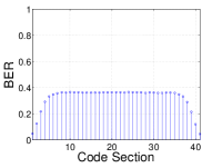
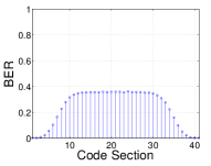
(a)	(b)
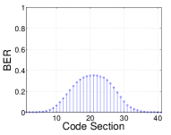
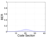
(c)	(d)

Figure 3: Bit Error Probability per code section during the decoding process for $\ell=5$ (a), $\ell=30$ (b), $\ell=70$ (c) and $\ell=110$ (d) for a convolutional code with $L=20$, $M=1024$ and $\epsilon=0.44$.

On the other hand, for ${\epsilon}\geq\epsilon^{\text{BP}}(l,r)$, we expect that the number of required iterations scales linearly in $L$: the “decoding wave” starts at the boundaries and moves at a constant speed towards the middle [Lentmaier10]. This can be seen in Fig. 3, where we plot the bit error rate (BER) measured in each section of a $(l=3,r=6,L=20,M=1024)$ ensemble after $\ell=5$ (a), $\ell=30$ (b), $\ell=70$ (c) and $\ell=110$ (d) iterations for a channel parameter of ${\epsilon}=0.44$. In Fig. 4 we plot $\varphi(\ell,\epsilon,L,M)$ for $L=5,10,20$, $M=256,512$ and $\epsilon=0.44$. We have averaged over $50$ code samples. First observe that the distribution moves to the right with $L$ and we can see that the mean of the distributions scales linearly in $L$ – so the larger $L$ the more iterations we need. Further, as $M$ increases, the distribution concentrates around its mean. This means that for large $M$ most instances decode with a number of iterations which is close to the expected value. However, the distributions are heavy-tailed. I.e., over a large interval the curves are approximately straight lines, which indicates that over this range they follow a power law, i.e., they have the form $\ell^{\alpha}\beta$ for some non-negative constant $\alpha$ and $\beta$. Operationally this means that, with non-negligible probability, an instance takes many more iterations to decode as it is typical. The last two conclusions are quite similar to what can be observed for standard LDPC ensembles, see [Urbanke08-2]. One strategy to deal with the linear increase of the decoding complexity for very large chain lengths is the application of a windowed decoder [Papaleo10].

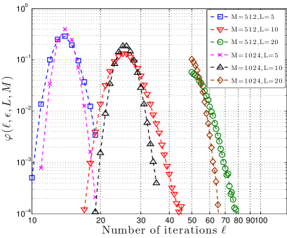
Figure 4: Distribution for the BP required number of iterations, for a regular (3,6) code for $L\in\{5,10,20\}$ and $M\in\{512,1024\}$ and $\epsilon=0.465$.

IV Scaling Behavior

Let us now investigate for what scalings $L=f(M)$ the threshold saturation effect appears. We have run a large set of simulations for various scaling functions $f(M)$ and a regular $(l,r)=(3,6)$ code has been used to construct the ensembles. The BP and MAP thresholds for this ensemble are, respectively, $\epsilon^{\text{BP}}(l,r)\approx 0.4294$ and $\epsilon^{\text{MAP}}(l,r)\approx 0.4815$. The BP decoder is run until all messages have converged (which always happens for the BEC). We choose a $(l,r)=(3,6)$ code to better illustrate the effect of the error floor in the scaling since regular codes with larger degrees, e.g., a $(5,10)$ regular ensemble, have much lower error floors. Our current aim however is not to construct optimal codes but to illustrate some typical effects. For each $(L,M)$ pair we only consider one single sample, randomly taken from the ensemble, as described in Section II. For each $\epsilon$ value and fixed code, we consider $10^{5}$ transmitted codewords.

IV-A Fixed $L$, Increasing $M$

Consider first the case of constant $f(M)$. Since this is the regime used for the DE analysis, we know that the limiting performance $M\rightarrow\infty$ is given by (2). We can get a negligible error probability as long as we are operating below the threshold $\epsilon^{\text{MAP}}(l,r)$. In Fig. 5, we represent the bit error probability when $L$ is fixed to $100$. As expected, the curves become steeper as we increase $M$. Note that the curves show an error floor. As we discuss in more detail in Section V, this error floor is due to the fact that the ratio $L/M^{l-2}$ is relatively large for most of these cases.

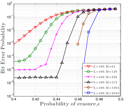
Figure 5: Bit Error probability $P_{b}^{\ell}(\epsilon,l,r,L)$ for a $(l=3,r=6,L,M)$ code. $L$ is fixed to 100.

IV-B Fixed $M$, Increasing $L$

Let us now look at the other extreme. i.e., we fix $M$ to some constant $M_{0}>0$ and let $L$ grow. Clearly, in this regime we do not expect to see the same threshold saturation phenomenon. If we consider $P_{b}^{\ell=\infty}(\epsilon,l,r,L,M_{0})$ and if we increase $L$ then we expect this error probability to be monotonically increasing in $L$ since the longer the chain the higher the chance that the “decoding wave” gets stuck before reaching the middle. In Fig. 6, we plot the error probability for the case $M_{0}=512$. As expected, the error probability is indeed monotonically increasing in $L$ and it seems to converge to a limiting curve. The determination of this limiting curve is an interesting open problem.

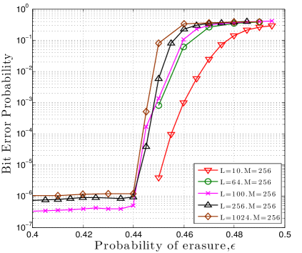
Figure 6: Bit Error probability $P_{b}^{\ell}(\epsilon,l,r,L)$ for a $(l=3,r=6,L,M)$ code. $M$ is fixed to 256.

IV-C $L$ as a general function of $M$

Now where we have investigated the two limiting cases it is of interest to scale both $M$ and $L$ together. At what scaling does the behavior change? In Fig. 7 and Fig. 8, we test the scaling functions $L=M/2$ and $L=(M/2)^{2}$. In Fig. 8, we have included, in dashed lines, the asymptotic ensemble error floor derived in Section V. For both scaling functions the performance improves with $M$, although in Fig. 8 the speed of improvement is slower. Indeed, it seems that in both cases the asymptotic threshold still is $\epsilon^{\text{MAP}}(l,r)$. This illustrates that the threshold saturation phenomenon is quite robust and general. Due to the large $L/M^{l-2}$ values, we observe large error floor levels in both cases. Finally, in Fig. 9 we plot the performance of an extreme scenario, where $L$ scales exponentially with $M$. The performance now worsens with $L$, similarly to the case considered in Section IV-B. A back of the envelope calculation, proposed to us by Andrea Montanari, suggests that an exponential scaling relationship is exactly the boundary – for a subexponential growth of $L$ as a function of $M$ we expect the threshold phenomenon to happen whereas for super-exponential growths we expect it not to occur.

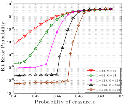
Figure 7: Bit Error probability $P_{b}^{\ell}(\epsilon,l,r,L)$ for a $(l=3,r=6,L,M)$ code. $L$ is equal to $M/2$.

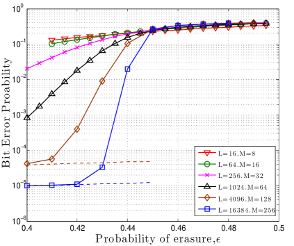
Figure 8: Bit Error probability $P_{b}^{\ell}(\epsilon,l,r,L)$ for a $(l=3,r=6,L,M)$ code. $L$ is equal to $(M/2)^{2}$. In dashed lines, we represent the asymptotic ensemble error floor in (LABEL:eq:ExBER) for $M=128$ and $M=256$.

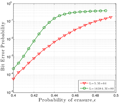
Figure 9: Bit Error probability $P_{b}^{\ell}(\epsilon,l,r,L)$ for a $(l=3,r=6,L,M)$ code. $L$ scales exponentially with $M$.

Let us summarize. The threshold saturation phenomenon happens empirically over a very wide range of scalings of $L$ with respect to $M$ and far beyond what theory currently can predict. This is of comfort to the code designer in the field and a challenge for any theoretician.

V Error Floor

In many of the former simulations, we have seen the occurrence of error floors. Let us now quickly discuss how this error floor can be analyzed. To simplify matters, we only consider codewords/stopping sets of weight two since codewords/stopping sets of higher weight vanish (in $M$) at a much higher rate.

Lemma 1 (Convergence to Poisson Distribution)

Consider an LDPCC ensemble $(l,r=kl,L,M)$. Let $\mathcal{C}$ be a code sample and ${N_{2}^{H}}$ be the number codewords with Hamming weight two in $\mathcal{C}$. Assume that the code is chosen randomly with a uniform probability from the ensemble. Then the distribution of ${N_{2}^{H}}$ converges (in $M$) to

$${N_{2}^{H}}\sim\textrm{Pois}\left(\lambda\right),\quad\lambda=k^{l-2}\binom{k}{2}\frac{(2L+1)}{M^{l-2}}\quad k\geq 2.$$ (7)

Proof:

Note that a codeword of weight two is only formed by two variables in the same section, see Fig. 2, that share the same set of $l$ check nodes. Since there are $(M/k)$ check nodes per section, this happens with probability $p=(M/k)^{-l}$. In each section, we count $\binom{k}{2}(M/k)^{2}$ pairs of variables that can form a weight two codeword. Therefore, in a graph with $(2L+1)$ sections, the expected number of such codewords converges to $\lambda=(2L+1)\binom{k}{2}(M/k)^{2}p$. That the distribution converges to a Poisson distribution follows by standard arguments as in the case of uncoupled LDPC ensembles, see [Urbanke08-2]. ∎