An inhomogeneous toy model of the quantum gravity with explicitly evolvable observables

Abstract

An inhomogeneous (1+1)-dimensional model of the quantum gravity is considered. It is found, that this model corresponds to a string propagating against some curved background space. The quantization scheme including the Wheeler-DeWitt equation and the “particle on a sphere” type of the gauge condition is suggested. In the quantization scheme considered, the “problem of time” is solved by building of the quasi-Heisenberg operators acting in a space of solutions of the Wheeler-DeWitt equation and the normalization of the wave function corresponds to the Klein-Gordon type. To analyze the physical consequences of the scheme, a (1+1)-dimensional background space is considered for which a classical solution is found and quantized. The obtained estimations show the way to solution of the cosmological constant problem, which consists in compensation of the zero-point oscillations of the matter fields by the quantum oscillations of the scale factor. Along with such a compensation, a slow global evolution of a background corresponding to an universe expansion exists.

1 Introduction

The generally covariant canonical quantization of gravity has been proposed in [1, 2]. As a result, the well-known Wheeler-DeWitt (WDW) equation has been obtained from the Hamiltonian formulation of the general relativity theory (GR). The main problem preventing a further development of the canonical quantum gravity is an absence of explicit evolution that is a consequence of the Hamiltonian constraint (e.g., see [3, 4, 5, 6, 7]).

It is well-known, that the string theory [8, 9] has the Hamiltonian constraint, as well, but it does not face the “problem of time”. The point is that either the equations of motion are quantized (in the covariant approach) or the time-dependent gauges are used (in the light-cone approach) in the quantized string theory. From the other hand, the WDW equation is not used in the string theory although this possibility was discussed [9, 10]. A thought suggests itself, that the quantization of the equations of motion can be suitable also in the quantum gravity and, at the same time, the WDW equation can make sense for some kinds of strings.

In our previous works [11, 12], we have demonstrated the quantization scheme including both quantization of the equations of motion and the WDW equation for a minisuperspace model. The ideology of quantization is quite similar to that in the string theory, where some time-dependent gauge is used, except the fact that the gauge is not imposed at all times but only at the initial instant and thereafter it is permissible for operators to evolve in accordance with the equations of motion. Another distinctive feature of the method proposed is that the evolvable operators (so-called, quasi-Heisenberg operators) act in a space of the solutions of the WDW equation, which are normalized in the Klein-Gordon style. Here we extend the quasi-Heisenberg quantization scheme to the string in the curved background space that can be treated as an inhomogeneous (1+1)-dimensional toy model of the quantum gravity.

2 Model of a spatially inhomogeneous gravity

We shall follow a heuristic method to obtain a spatially inhomogeneous gravity model in two space-time dimensions. The Lagrangian for a gravitation and a scalar field $\phi$ can be written in the form

$$S=-\frac{M_{p}^{2}}{12}\int\mathcal{G}\sqrt{-g}\,d^{4}x+\frac{1}{2}\int\biggl{(}\partial_{\mu}\phi\,g^{\mu\nu}\partial_{\nu}\phi-m^{2}\phi^{2}\biggr{)}\sqrt{-g}\,d^{4}x,$$ (1)

where $\mathcal{G}=g^{\alpha\beta}\left(\Gamma_{\alpha\nu}^{\rho}\Gamma_{\beta\rho}^{\nu}-\Gamma_{\alpha\beta}^{\nu}\Gamma_{\nu\rho}^{\rho}\right)$ [13] and $M_{p}$ is the Planck mass, which is chosen as $M_{p}=\sqrt{\frac{3}{4\pi G}}$.

If one restricts a metric to the form

$$ds^{2}=a^{2}(\tau,\bm{r})(N^{2}(\tau,\bm{r})d\tau^{2}-d\bm{r}^{2}),$$

the resulting Lagrangian becomes:

$$\eqalign{L=\frac{1}{2}\int\biggl{\{}N\left(-\frac{M_{p}^{2}\,a^{\prime 2}}{N^{2}}+M_{p}^{2}(\bm{\nabla}a)^{2}-\frac{2M_{p}^{2}}{3}\bm{\nabla}\cdot(a\bm{\nabla}a)+a^{2}\biggl{(}\frac{\phi^{\prime 2}}{N^{2}}-(\bm{\nabla}\phi)^{2}\right)\\ ~{}~{}~{}~{}~{}~{}~{}~{}~{}~{}~{}~{}~{}~{}~{}~{}~{}~{}~{}~{}~{}~{}~{}~{}~{}~{}~{}~{}~{}~{}~{}~{}~{}~{}~{}~{}~{}~{}~{}~{}~{}-m^{2}a^{4}\phi^{2}\biggr{)}+\frac{2M_{p}^{2}}{3}\bm{\nabla}\cdot(a\bm{\nabla}a\,N)\biggr{\}}d^{3}\bm{r},}$$

where a prime denotes a derivative over the time.

The last term in Eq. (2) can be omitted as a total divergence. The variation with respect to $N$ gives the Hamiltonian constraint:

$$\mathcal{H}=\frac{1}{2}\left(-\frac{M_{p}^{2}a^{\prime 2}}{N^{2}}-M_{p}^{2}(\bm{\nabla}a)^{2}+\frac{2M_{p}^{2}}{3}\bm{\nabla}\cdot(a\bm{\nabla}a)+a^{2}\frac{\phi^{\prime 2}}{N^{2}}+a^{2}(\bm{\nabla}\phi)^{2}+m^{2}a^{4}\phi^{2}\right)=0.$$ (2)

Hereinafter, let us consider the conformal time gauge $N=1$. The term $-\frac{2M_{p}^{2}}{3}\bm{\nabla}\cdot(a\bm{\nabla}a)$ in Eq. (2) does not affect the equations of motion, which have the form

$$M_{p}^{2}a^{\prime\prime}-M_{p}^{2}\bm{\nabla}^{2}a+a\left(\phi^{\prime\,2}-(\bm{\nabla}\phi)^{2}\right)-2a^{3}m^{2}\phi^{2}=0,$$ (3)

$$\phi^{\prime\prime}+2\frac{a^{\prime}}{a}\phi^{\prime}-\frac{1}{a^{2}}\bm{\nabla}\cdot(a^{2}\bm{\nabla}\phi)+a^{2}m^{2}\phi=0.$$ (4)

Then, the time evolution of the Hamiltonian constraint can be expressed as:

$$\partial_{\tau}\mathcal{H}=\bm{\nabla}\cdot\mathcal{\bm{P}},$$ (5)

where the momentum constraint is $\mathcal{\bm{P}}=-M_{p}^{2}a^{\prime}\bm{\nabla}a+a^{2}\phi^{\prime}\bm{\nabla}\phi$. On the contrary, the time derivative of the momentum constraint is not expressed through $\mathcal{H}$ and $\mathcal{\bm{P}}$. Thus, this system does not belong to the fist kind one [14, 15, 16] unlike GR. Nevertheless, if one considers an (1+1)-dimensional analog of (2) with a massless scalar field

$$L=\frac{1}{2}\int N\left(-\frac{M_{p}^{2}a^{\prime 2}}{N^{2}}+M_{p}^{2}\left(\frac{\partial a}{\partial\sigma}\right)^{2}+a^{2}\left(\frac{{\phi^{\prime 2}}}{N^{2}}-\left(\frac{\partial\phi}{\partial\sigma}\right)^{2}\right)\right)d\sigma,$$ (6)

($\sigma$ denotes the only spatial variable), the Lagrangian (6) proves to correspond to a string propagating against some curved background space and, thus, it gives a completely self-consistent system of constraints like that of GR.

3 Connection with the string theory

It is believed that the superstring theory shall include the GR. Nevertheless, one may try to connect the string theory with the GR directly by means of reduction of the GR Lagrangian on assumption that the space-time has some symmetry [17]. In the present work, we shall demonstrate that the Lagrangian (6) with a nonuniform scale factor describes a string against a curved background. Such a string model can be interpreted as an inhomogeneous toy model for the quantum gravity.

Let us write the standard form of action for a bosonic string [8] in a background space

$$S=\int d^{2}\xi\sqrt{-h}\,h^{\alpha\beta}(\xi)\partial_{\alpha}X^{\mu}\partial_{\beta}X^{\nu}g_{\mu\nu}(X(\xi)),$$ (7)

where $\xi=\{\tau,\sigma\}$. The metric tensor $h_{\alpha\beta}(\xi)$ describes the intrinsic geometry of a (1+1)-dimensional manifold and $g_{\mu\nu}(X(\xi))$ describes the geometry of a background space. Variation with respect to $h_{\alpha\beta}(\xi)$ leads to the constraints [8]:

$$\frac{\delta S}{\delta h_{\alpha\beta}}\equiv T_{\alpha\beta}=\partial_{\alpha}X^{\mu}\partial_{\beta}X^{\nu}g_{\mu\nu}(X)-\frac{1}{2}h_{\alpha\beta}h^{\eta\kappa}\partial_{\eta}X^{\mu}\partial_{\kappa}X^{\nu}\,g_{\mu\nu}(X)=0.$$ (8)

If one takes $X^{\mu}=\{a,\phi\}$, the metric tensor $h_{\mu\nu}$ in the form of

$$h=\left(\begin{array}[]{cc}-N^{2}+N_{1}^{2}&N_{1}\\ N_{1}&1\end{array}\right),$$

and the metric tensor $g_{\mu\nu}(X)$ of a background space as

$$g=\left(\begin{array}[]{cc}M_{p}^{2}&0\\ 0&-a^{2}\end{array}\right),$$ (9)

it results in the Lagrangian for the (1+1)-dimensional model

$$L=\int\Biggl{(}\frac{M_{p}^{2}}{2}\partial_{\sigma}a^{2}\left({N}-\frac{{N_{1}}^{2}}{{N}}\right)+M_{p}^{2}\frac{\partial_{\sigma}a\,a^{\prime}{N_{1}}}{{N}}-M_{p}^{2}\frac{a^{\prime 2}}{2{N}}$$

$$~{}~{}~{}~{}~{}~{}~{}~{}~{}~{}~{}~{}~{}~{}-\frac{a^{2}{N_{1}}\partial_{\sigma}\phi\,\phi^{\prime}}{{N}}+\frac{1}{2}a^{2}\,\partial_{\sigma}\phi^{2}\left(\frac{{N_{1}}^{2}}{{N}}-{N}\right)+\frac{a^{2}\phi^{\prime 2}}{2{N}}\Biggr{)}d\sigma.$$ (10)

The substitutions of $N_{1}=0$ and $N=1$ into (10) reduces it to (6). Thus, the constraints (8) become the Hamiltonian and momentum constraints of the model considered.

In a more general case, one may consider a number of scalar fields besides the scale factor $a$, i.e $X=\{a,\phi_{1},\phi_{2},\dots\phi_{N}\}$ and take the background metric tensor

$$g_{\mu\nu}(X)=\mbox{diag}\{M_{p}^{2},-a^{2},-a^{2}\dots\}.$$ (11)

Let us denote $\alpha=\ln a$ and rewrite the Lagrangian (6) in the terms of $\alpha$ and a set of scalar fields :

$$L=\frac{1}{2}\int e^{2\alpha}\left(-M_{p}^{2}\alpha^{\prime 2}+\bm{\phi}^{\prime 2}+M_{p}^{2}(\partial_{\sigma}\alpha)^{2}-(\partial_{\sigma}\bm{\phi})^{2}\right)d\sigma=0,$$ (12)

where $\bm{\phi}=\{\phi_{1},\phi_{2}\dots\phi_{N}\}$. The relevant Hamiltonian and momentum constraints (8), written in the terms of momentums $\bm{\pi}(\sigma)\equiv\frac{\delta L}{\delta{\bm{\phi}^{\prime}(\sigma)}}=e^{2\alpha}\bm{\phi}^{\prime}$ and $p_{\alpha}(\sigma)\equiv-\frac{\delta L}{\delta\alpha^{\prime}(\sigma)}=M_{p}^{2}\,e^{2\alpha}\alpha^{\prime}$ take the form of

$$\mathcal{H}(\sigma)=\frac{1}{2}e^{-2\alpha}\left(-p_{\alpha}^{2}/M_{p}^{2}+\bm{\pi}^{2}\right)+e^{2\alpha}\left(-M_{p}^{2}(\partial_{\sigma}\alpha)^{2}+(\partial_{\sigma}\bm{\phi})^{2}\right)=0,$$ (13)

$$\mathcal{P}(\sigma)=-p_{\alpha}\partial_{\sigma}\alpha+\bm{\pi}\partial_{\sigma}\bm{\phi}=0.$$ (14)

The constraints algebra demonstrates that there are no new constraints:

$$\{\mathcal{H}(\sigma),\mathcal{H}(\sigma^{\prime})\}=(\mathcal{P}(\sigma)+\mathcal{P}(\sigma^{\prime}))\delta^{\prime}(\sigma-\sigma^{\prime}),$$

$$\{\mathcal{P}(\sigma),\mathcal{P}(\sigma^{\prime})\}=(\mathcal{P}(\sigma)+\mathcal{P}(\sigma^{\prime}))\delta^{\prime}(\sigma-\sigma^{\prime}),$$

$$\{\mathcal{P}(\sigma),\mathcal{H}(\sigma^{\prime})\}=(\mathcal{H}(\sigma)+\mathcal{H}(\sigma^{\prime}))\delta^{\prime}(\sigma-\sigma^{\prime}),$$

where $\delta^{\prime}(\sigma-\sigma^{\prime})$ is the derivative of the Dirac delta-function, and the Poisson brackets are implied:

$$\eqalign{\{A(\sigma),B(\sigma^{\prime})\}=\int\Biggl{(}-\frac{\delta A(\sigma)}{\delta p_{\alpha}(\xi)}\frac{\delta B(\sigma^{\prime})}{\delta\alpha(\xi)}+\frac{\delta A(\sigma)}{\delta\alpha(\xi)}\frac{\delta B(\sigma^{\prime})}{\delta p_{\alpha}(\xi)}\\ +\sum_{j}^{N}\frac{\delta A(\sigma)}{\delta\pi_{j}(\xi)}\frac{\delta B(\sigma^{\prime})}{\delta\phi_{j}(\xi)}-\frac{\delta A(\sigma)}{\delta\phi_{j}(\xi)}\frac{\delta B(\sigma^{\prime})}{\delta\pi_{j}(\xi)}\Biggr{)}d\xi}$$ (15)

.

The next step is the quantization of the model presented. It is known, that the string theory demands $X^{\mu}$ to have the critical dimension, which is of 26 for a bosonic string. Nevertheless, even for the critical dimension, one cannot expect that the string theory gives a satisfactory quantization of the model against a curved background. The point is that the string theory provides a consistent quantization only if the Ricci tensor $R_{\mu\nu}(X)$ of the background metric $g_{\mu\nu}(X)$ equals to zero [8, 18]. For $g_{\mu\nu}$ given by (11), it is nonzero if the dimension of $X^{\mu}$ is higher than two (the scalar curvature is constant in the case considered). However, it was stated [8, 18] that an inclusion of some other fields (e.g., dilaton) leads to the standard Einstein equations $R_{\mu\nu}(X)\neq 0$ for the background metric and it can be considered as a new principle of derivation of the Einstein equations [18].

It should be noted, that the string representation arises in our paper in a quite different context than the ordinary one (in particular, as used in [17]). In our model the background space is an isospin-like space determined by the number of scalar fields (matter degrees of freedom, whereas the physical space, where the observers and detectors could be situated) is a $(\tau,\sigma)-$ space. On the contrary, the ordinary string theory considers a background space as “physical” one, whereas a $(\tau,\sigma)-$space corresponds to “internal degrees of freedom”. Thus, the quantization resulting in the dimension constraints for a background space (i.e., for a number of matter fields in our case) can be hardly acceptable in the model considered. In the next section, we shall present the quantization scheme for $R_{\mu\nu}(X)\neq 0$ and a background space without any dimension constraints.

4 Quantization

4.1 Relativistic “fluid” on a sphere

The minisuperspace model presented in [11, 12] demonstrates that the quasi-Heisenberg quantization consists in the following: one has to set the initial values for the operators, which evolve in accordance with the operator equations of motion. The question is to construct the representation for these operators and the space where they act. In our approach this problem is solved by consideration of the Hamiltonian constraint as the WDW equation and choice of the plane $a=0$ for normalization of a wave function in the Klein-Gordon style. In the general case, the momentum constraint is also should be taken into account. This requires to impose one additional gauge condition. The light cone gauge [8, 19] is widely used in the string theory. Since it contains necessarily a nonzero mean momentum, it is hardly acceptable for our isotropic cosmological-like model. Thus, it is necessary to propose some new gauge. The hint arises from the form of the momentum constraint, which reminds that in the theory of a particle moving on a sphere [20, 21, 22, 23].

At first, let us consider a simpler problem described by the Hamiltonian

$$H=\frac{1}{2}(-p_{0}^{2}+\bm{p}^{2})=0,$$ (16)

which is similar to that of a massless relativistic particle.

The analog of the momentum constraint can be writing as

$$P=-x_{0}p_{0}+\bm{p}\,\bm{r}=0,$$ (17)

where $\bm{p}=\{p_{1},p_{2}\dots p_{N}\}$, $\bm{r}=\{x_{1},x_{2}\dots x_{N}\}$.

The constraint algebra is

$$\{H,P\}=-\frac{\partial H}{\partial p_{0}}\frac{\partial P}{\partial x_{0}}+\frac{\partial H}{\partial x_{0}}\frac{\partial P}{\partial p_{0}}+\frac{\partial H}{\partial\bm{p}}\frac{\partial P}{\partial\bm{r}}-\frac{\partial H}{\partial\bm{r}}\frac{\partial P}{\partial\bm{p}}=2H.$$ (18)

Let us take the gauge condition in the form of

$${\mathcal{A}}=-x_{0}^{2}+\bm{r}^{2}-R^{2}=0,$$ (19)

where $R$ is some constant.

The first step is to formulate the WDW equation. The momentum constraint and the gauge condition allow excluding one of the degrees of freedom, for instance, the coordinate $x_{N}$ and the momentum $p_{N}$. Let’s denote $\bm{\Pi}=\{p_{1},p_{2}\dots p_{N-1}\}$ and $\bm{\mathcal{X}}=\{x_{1},x_{2}\dots x_{N-1}\}$. Then

$$x_{N}=\Theta\,\sqrt{R^{2}+x_{0}^{2}-\bm{\mathcal{X}}^{2}},$$ (20)

$$p_{N}=\Theta\,(x_{0}p_{0}-\bm{\mathcal{X}}\,\bm{\Pi})/\sqrt{R^{2}+x_{0}^{2}-\bm{\mathcal{X}}^{2}},$$ (21)

where $\Theta$ takes the values $\pm 1$. The coordinates $\bm{\mathcal{X}}$ and $\Theta$ correspond to the vertical plane projection of a sphere shown in Fig. 1. The value $\Theta=1$ corresponds to the upper semisphere and $\Theta=-1$ corresponds to the lower one.

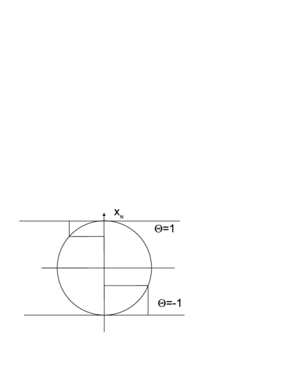
Figure 1: Vertical plane projections of the points on a sphere.

Substitution of the above quantities into (16) results in

$$-p_{0}^{2}+\bm{\Pi}^{2}+\frac{(p_{0}x_{0}-\bm{\Pi}\bm{\mathcal{X}})^{2}}{R^{2}+x_{0}^{2}-\bm{\mathcal{X}}^{2}}=0.$$ (22)

Further, we shall take an interest only in the region of $x_{0}\rightarrow 0$ and $R\rightarrow\infty$, where the asymptotic of Eq. (22) takes the form of

$$-p_{0}^{2}+\bm{\Pi}^{2}=0.$$ (23)

Obtaining of the WDW equation consists in the postulation of

$$p_{0}=i\frac{\partial}{\partial x_{0}},~{}~{}~{}~{}~{}\bm{\Pi}=-i\frac{\partial}{\partial\bm{\mathcal{X}}},$$

that results in

$$\left(\frac{\partial^{2}}{\partial x_{0}^{2}}-\frac{\partial^{2}}{\partial\bm{\mathcal{X}}^{2}}\right)\Psi(x_{0},\Theta,\bm{\mathcal{X}})=0.$$ (24)

The wave packet solution [11, 12] is

$$\Psi(x_{0},\bm{\mathcal{X}},\Theta)=\int c(\bm{k},\Theta)e^{-i|\bm{k}|x_{0}+i\bm{k}\bm{\mathcal{X}}}d^{N-1}\bm{k},$$ (25)

where $c(\bm{k},\Theta)=c_{0}(\bm{k})+\Theta\,c_{1}(\bm{k})$.

A mean value of an arbitrary operator $A$ is given by [11, 12, 28]

$$<\Psi|\hat{A}(x_{0},\Theta,\bm{\mathcal{X}},\hat{\bm{\Pi}})|\Psi>=\frac{i}{2}\sum_{\Theta=\pm 1}\int\Biggl{(}\Psi^{*}(x_{0},\Theta,\bm{\mathcal{X}}){\hat{D}^{1/4}}\hat{A}\,{\hat{D}^{-1/4}}\frac{\partial}{\partial x_{0}}\Psi(x_{0},\Theta,\bm{\mathcal{X}})$$

$$-\left(\frac{\partial}{\partial x_{0}}\Psi^{*}(x_{0},\Theta,\bm{\mathcal{X}})\right){\hat{D}^{-1/4}}\hat{A}\,{\hat{D}^{1/4}}\,\Psi(x_{0},\Theta,\bm{\mathcal{X}})\Biggr{)}d^{N-1}\bm{\mathcal{X}}\biggr{|}_{\,x_{0}\rightarrow 0},$$ (26)

where $\hat{D}$ is the operator $\hat{D}=-\frac{\partial^{2}}{\partial\bm{\mathcal{X}}^{2}}$.

In the momentum representation of the wave function

$$\Psi(x_{0},\bm{\mathcal{X}},\Theta)=\int c(\bm{k},\Theta)e^{-i|\bm{k}|x_{0}+i\bm{k}\bm{\mathcal{X}}}d^{N-1}\bm{k},$$

the mean value of an operator is given as

$$<\hat{A}>=\sum_{\Theta=\pm 1}\int c^{*}(\bm{k},\Theta)e^{i|\bm{k}|x_{0}}\hat{A}(x_{0},\Theta,i\frac{\partial}{\partial\bm{k}},{\bm{k}})\,c(\bm{k},\Theta)e^{-i|\bm{k}|x_{0}}\,d^{N-1}\bm{k}\biggr{|}_{\,x_{0}\rightarrow 0}.$$ (27)

The equations of motion follow from Eq. (16) via the Hamilton-Jacobi equations $\frac{dx_{i}}{d\tau}=\{H,x_{i}\}$, $\frac{dp_{i}}{d\tau}=\{H,p_{i}\}$ and take the form of

$$\frac{dx_{i}}{d\tau}=p_{i},~{}~{}~{}\frac{dx_{0}}{d\tau}=p_{0},~{}~{}~{}\frac{dp_{i}}{d\tau}=0,~{}~{}~{}\frac{dp_{0}}{d\tau}=0.$$ (28)

We shall consider them as the operator equations. For more complicated systems, some operator ordering could be needed.

Now one has to assign the initial values for the quasi-Heisenberg operators. In our model, they are build according to the Dirac rule for the full set of constraints and gauge conditions but only at the initial moment of the proper time $\tau$. The full set of constraints at $\tau=0$ is $F=\{H,P,{\mathcal{A}},{\mathcal{B}}\}$, where the gauge condition ${\mathcal{B}}=x_{0}$ suggests $x_{0}(0)=0$. This gauge condition is taken to adjust the commutation rules for the initial values of quasi-Heisenberg operators to the hyperplane $x_{0}=0$, where a wave function is normalized in the Klein-Gordon style in accordance with Eqs. (26), (27).

The Dirac matrix consists of the Poisson brackets of constraints and the gauge conditions

$$M_{\alpha\beta}=\{F_{\alpha},F_{\beta}\}=-\frac{\partial F_{\alpha}}{\partial p_{0}}\frac{\partial F_{\beta}}{\partial x_{0}}+\frac{\partial F_{\alpha}}{\partial x_{0}}\frac{\partial F_{\beta}}{\partial p_{0}}+\sum_{j}^{N}\frac{\partial F_{\alpha}}{\partial p_{j}}\frac{\partial F_{\beta}}{\partial x_{j}}-\frac{\partial F_{\alpha}}{\partial x_{j}}\frac{\partial F_{\beta}}{\partial p_{j}},$$ (29)

that leads to

$$M=\left(\begin{array}[]{cccc}0&0&0&p_{0}\\ 0&0&2R^{2}&0\\ 0&-2R^{2}&0&0\\ -p_{0}&0&0&0\end{array}\right).$$ (30)

The inverse matrix $M^{-1}$ is evident and we can calculate the Dirac brackets [14, 15, 16]:

$$\{p_{i},x_{j}\}_{D}=\{p_{i},x_{j}\}-\sum_{\alpha,\beta}\{p_{i},F_{\alpha}\}M^{-1}_{\alpha\beta}\{F_{\beta},x_{j}\}.$$ (31)

The corresponding commutation relations at $\tau=0$ can be obtained by multiplication of the right hand side of Eq. (31) by $(-i)$ that results in

$$\eqalign{\left[\hat{p}_{l}(0),\hat{x}_{j}(0)\right]=-i\left(\delta_{lj}-\frac{\hat{x}_{l}(0)\hat{x}_{j}(0)}{R^{2}}\right),\cr\left[\hat{x}_{i}(0),\hat{x}_{j}(0)\right]=0,~{}~{}~{}~{}\left[\hat{p}_{l}(0),\hat{p}_{j}(0)\right]=\frac{-i}{R^{2}}S\left(\hat{p}_{l}(0)\hat{x}_{j}(0)-\hat{x}_{l}(0)\hat{p}_{j}(0)\right),\cr\left[\hat{p}_{0}^{2}(0),\hat{x}_{j}(0)\right]=-i\frac{2}{R^{2}}S\left(\hat{p}_{j}(0)\sum_{m\neq j}^{N}\hat{x}_{m}^{2}(0)-\hat{x}_{j}(0)\sum_{m\neq j}^{N}\hat{p}_{m}(0)\hat{x}_{m}(0)\right),\cr\left[\hat{p}_{0}^{2}(0),\hat{p}_{j}(0)\right]=-i\frac{2}{R^{2}}S\left(\hat{x}_{j}(0)\sum_{m\neq j}^{N}\hat{p}_{m}^{2}(0)-\hat{p}_{j}(0)\sum_{m\neq j}^{N}\hat{p}_{m}(0)\hat{x}_{m}(0)\right),}$$ (32)

where symbol $S$ denotes symmetrization of the noncommuting operators, i.e. $S(\hat{A}\hat{B})=\frac{1}{2}(\hat{A}\hat{B}+\hat{B}\hat{A})$ or $S(\hat{A}\hat{B}\hat{C})=\frac{1}{6}(\hat{A}\hat{B}\hat{C}+\hat{B}\hat{A}\hat{C}+\hat{A}\hat{C}\hat{B}+\dots)$. Certainly, the quantity $\hat{x}_{0}(0)=0$ is $c$-number and commutes with all operators.

Realization of the commutation relations is represented as

$$\eqalign{\hat{x}_{j}(0)=x_{j},~{}~{}~{}~{}~{}\hat{p}_{j}(0)=-i\left(\frac{\partial}{\partial x_{j}}-\frac{1}{R^{2}}S\left(x_{j}\left(\bm{\mathcal{X}}\frac{\partial}{\partial\bm{\mathcal{X}}}\right)\right)\right),~{}~{}~{}~{}j\in\{1,N-1\},\\ \hat{x}_{N}(0)=\Theta\sqrt{R^{2}-\bm{\mathcal{X}}^{2}},~{}~{}~{}~{}\hat{p}_{N}(0)=i\,S\left(\frac{\Theta\sqrt{R^{2}-\bm{\mathcal{X}}^{2}}}{R^{2}}\left(\bm{\mathcal{X}}\frac{\partial}{\partial\bm{\mathcal{X}}}\right)\right),\\ \hat{p}_{0}(0)=\sqrt{\sum_{j=1}^{N}\hat{p}_{j}^{2}(0)}.}$$ (33)

Let us emphasize, that all commutation relations and constraints are satisfied as the operator equalities (i.e. strongly) at the initial time if the symmetrized quantum version of $\hat{\mathcal{P}}(0)=S\left(\sum_{j=1}^{N}\hat{p}_{j}(0)\hat{x}_{j}(0)\right)\$ is implied for the ${\mathcal{P}}$ constraint.

Now one can solve the equations of motion (28) with the above initial conditions (33) and calculate the mean values of operators according to (26), (27).

It is essential, that Eqs. (33) can be simplified in the vicinity of $R\rightarrow\infty$:

$$\eqalign{\hat{x}_{j}(0)=x_{j},~{}~{}~{}~{}\hat{p}_{j}(0)=-i\frac{\partial}{\partial x_{j}},~{}~{}~{}~{}j\in\{1,N-1\},\\ \\ \hat{x}_{N}=\Theta\,R,~{}~{}~{}~{}\hat{p}_{N}(0)=i\,\frac{\Theta}{R}S\left(\bm{\mathcal{X}}\frac{\partial}{\partial\bm{\mathcal{X}}}\right).}$$ (34)

4.2 Quantization scheme for the string in a (1+N)-dimensional space

We intend to quantize the string in a curved background space by close analogy with the quantization of the “fluid” on a sphere. Let’s take the gauge condition in the form of

$${\mathcal{A}}=e^{2\alpha}\left(-M_{p}^{2}(\partial_{\sigma}\alpha)^{2}+(\partial_{\sigma}\bm{\phi})^{2}\right)-\Lambda^{2}=0,$$ (35)

where $\Lambda$ is some constant. In fact, we equal the part of Hamiltonian density to $\Lambda^{2}$ at the initial time.

Let’s $\bm{\Pi}=\{\pi_{1},\pi_{2}\dots\pi_{N-1}\}$, $\bm{\Phi}=\{\phi_{1},\phi_{2}\dots\phi_{N-1}\}$, then $\phi_{N}$ and $\pi_{N}$ are expressed through the momentum constraint (14) and the gauge condition (35) as

$$\partial_{\sigma}\phi_{N}(\sigma)=\Theta(\sigma)\sqrt{\Lambda^{2}e^{-2\alpha}+M_{p}^{2}(\partial_{\sigma}\alpha)^{2}-(\partial_{\sigma}\bm{\Phi})^{2}},$$ (36)

$$\pi_{N}(\sigma)=\Theta(\sigma)\frac{p_{\alpha}\partial_{\sigma}\alpha-\bm{\Pi}\partial_{\sigma}\bm{\Phi}}{\sqrt{\Lambda^{2}e^{-2\alpha}+M_{p}^{2}(\partial_{\sigma}\alpha)^{2}-(\partial_{\sigma}\bm{\Phi})^{2}}},$$ (37)

where $\Theta(\sigma)$ is the piecewise function taking the values $\pm 1$ such that $\Theta^{2}(\sigma)=1$.

Substitution of Eqs. (36),(37) to (13) leads to

$$e^{-2\alpha}\left(-p_{\alpha}^{2}/M_{p}^{2}+\bm{\Pi}^{2}+\frac{(p_{\alpha}\partial_{\sigma}\alpha-\bm{\Pi}\partial_{\sigma}\bm{\Phi})^{2}}{\Lambda^{2}e^{-2\alpha}+M_{p}^{2}(\partial_{\sigma}\alpha)^{2}-(\partial_{\sigma}\bm{\Phi})^{2}}\right)+\Lambda^{2}=0.$$ (38)

The asymptotic of Eq. (38) in the vicinity of $\alpha(\sigma)=\alpha_{0}\rightarrow-\infty$ is

$$e^{-2\alpha}\left(-p_{\alpha}^{2}/M_{p}^{2}+\bm{\Pi}^{2}\right)=0.$$ (39)

Hence, the quantization leads to the WDW equation

$$\left(\frac{1}{M_{p}^{2}}\frac{\delta^{2}}{\delta\alpha(\sigma)}-\left(\frac{\delta^{2}}{\delta^{2}\bm{\Phi}(\sigma)}\right)\right)\Psi[\alpha,\Theta,\bm{\Phi}]=0,$$ (40)

where $\frac{\delta}{\delta f(\sigma)}$ denotes the functional derivative.

The solution of Eq. (40) is the functional, which can be written as

$$\Psi[\alpha,\Theta,\bm{\Phi}]=\int C[\bm{\mathcal{K}},\Theta]\,e^{\int\left(-iM_{p}|\bm{\mathcal{K}}(\sigma)|\alpha(\sigma)+i\bm{\mathcal{K}}(\sigma)\bm{\Phi}(\sigma)\right)d\sigma}\,\mathcal{D}\bm{\mathcal{K}},$$ (41)

where $\int\dots\mathcal{D}\bm{\mathcal{K}}$ denotes a functional integral.

A mean value of an arbitrary operator can be evaluated as [11, 12, 28]

$$\eqalign{<\Psi|\hat{A}[\alpha,-i\frac{\delta}{\delta\bm{\Phi}},\bm{\Phi}]|\Psi>=i\int\biggl{(}\Psi^{*}[\alpha,\Theta,\bm{\Phi}]{\hat{D}^{1/4}}\hat{A}\,{\hat{D}^{-1/4}}\frac{\delta}{\delta\alpha(\sigma)}\Psi[\alpha,\Theta,\bm{\Phi}]\\ -\left(\frac{\delta}{\delta\alpha(\sigma)}\Psi^{*}[\alpha,\Theta,\bm{\Phi}]\right){\hat{D}^{-1/4}}\hat{A}\,{\hat{D}^{1/4}}\,\Psi[\alpha,\Theta,\bm{\Phi}]\biggr{)}\mathcal{D}\bm{\Phi}\,\mathcal{D}\Theta\biggr{|}_{\,\alpha(\sigma)=\alpha_{0}\rightarrow-\infty},}$$ (42)

where $\hat{D}(\sigma)=\frac{\delta^{2}}{\delta\bm{\Phi}^{2}(\sigma)}$.

The classical equations of motion obtained with the help of the Poisson brackets (15) are written as

$$\eqalign{\bm{\phi}^{\prime\prime}-\partial_{\sigma\sigma}\bm{\phi}+2\alpha^{\prime}\bm{\phi}^{\prime}-2\partial_{\sigma}\alpha\partial_{\sigma}\bm{\phi}=0,\\ M_{p}^{2}\alpha^{\prime\prime}-M_{p}^{2}\partial_{\sigma\sigma}\alpha+M_{p}^{2}\alpha^{\prime 2}-M_{p}^{2}(\partial_{\sigma}\alpha)^{2}+\bm{\phi}^{\prime 2}-(\partial_{\sigma}\bm{\phi})^{2}=0.}$$

Again, we shall consider these equations as the equations for the quasi-Heisenberg operators. One has to write the initial conditions for these equations and to choose the operator ordering in (4.2).

The additional gauge condition corresponding to the choice of the hyperplane $\mathcal{\alpha}(\sigma)=\alpha_{0}\rightarrow\infty$ in Eq. (42) is

$$\mathcal{B}=\alpha(0,\sigma)-\alpha_{0}=0,$$ (43)

where $\alpha_{0}$ is $c$-number which will be tended to minus infinity. Thus, there are two constraints $\mathcal{H}$, $\mathcal{P}$ given by Eqs. (13), (14) and two gauge conditions $\mathcal{A}$ , $\mathcal{B}$ given by Eqs. (35), (43), which are imposed at $\tau=0$. This allows calculating the Dirac brackets and obtaining the commutation relations at the initial moment of time. However, since it is necessary to know a representation of operators only in the vicinity of $\alpha_{0}\rightarrow-\infty$ where the radius of a sphere is $\Lambda e^{-\alpha_{0}}$ and , thereby, is infinitely large, one can write by analogy with (34)

$$\eqalign{\hat{\phi}_{j}(0,\sigma)={\phi}_{j}(\sigma),~{}~{}~{}~{}\hat{\pi}_{j}(0,\sigma)=-i\frac{\delta}{\delta\phi_{j}},~{}~{}~{}~{}j\in\{1,N-1\},\\ \hat{\phi}_{N}(0,\sigma)=\Delta(\sigma)\,\Lambda\,e^{-\alpha_{0}},~{}~{}~{}~{}\hat{\pi}_{N}(0,\sigma)=i\,\frac{\Theta(\sigma)}{\Lambda\,e^{-\alpha_{0}}}S\left(\bm{\Phi}(\sigma)\frac{\delta}{\delta\bm{\Phi}(\sigma)}\right),\\ \hat{\alpha}(0,\sigma)=\alpha_{0},~{}~{}~{}~{}~{}\hat{p}_{\alpha}(0,\sigma)=M_{p}\sqrt{\sum_{j=1}^{N}\hat{\pi}_{j}^{2}(0,\sigma)+\exp(2\alpha_{0})\Lambda^{2}},}$$ (44)

where $\Delta(\sigma)$ is the piece linear function such that $\Theta(\sigma)=\partial_{\sigma}\Delta(\sigma)$. The initial values of time derivatives of the scale factor logarithm and scalar field are expressed through the momentums given by (44) as $\hat{\alpha}^{\prime}(0,\sigma)=e^{-2\alpha_{0}}\hat{p}_{\alpha}(0,\sigma)$ and $\hat{\phi}_{j}^{\prime}(0,\sigma)=e^{-2\alpha_{0}}\hat{\pi}_{j}(0,\sigma)$.

The last step is to choose the operator ordering in the equations of motion (4.2). This problem is closely related to the constraint evolution. Heretofore, it was guessed that the constraints are satisfied only at the initial moment of time. One can ask whether the constraints will be satisfied during an evolution. Below we prove that if the symmetric (Weyl) ordering is chosen in the expressions for the constraints then there exists the operator ordering for the equations of motion, which preserves the constraints during an evolution.

One needs to extend the symmetrization operation $S$ used in (32) to a more general non-polynomial case [29, 30]. Let’s there is an arbitrary function $f(x_{1},x_{2},\cdots x_{n})$ of $n-$ variables. Then one can define the formal Fourier transform

$$\tilde{f}(\zeta_{1},\zeta_{2}\dots\zeta_{n})=\frac{1}{(2\pi)^{n}}\int f(x_{1},x_{2},\dots x_{n})e^{-i\left(x_{1}\zeta_{1}+x_{2}\zeta_{2}\dots x_{n}\zeta_{n}\right)}dx_{1}\dots dx_{n}.$$ (45)

The symmetrized function of the noncommuting operators $\hat{A}_{1},\dots\hat{A}_{n}$ is defined as

$$S(f(\hat{A}_{1},\hat{A}_{2}\dots\hat{A}_{n}))=\int\tilde{f}(\zeta_{1},\zeta_{2},\dots\zeta_{n})e^{i(\hat{A}_{1}\zeta_{1}+\hat{A}_{2}\zeta_{2}\dots\hat{A}_{n}\zeta_{n})}d\zeta_{1}\dots d\zeta_{n}.$$ (46)

The remarkable formula for the differentiation of the symmetrized function exists [30]

$$\frac{d}{dt}S(f(\hat{A}_{1}(t),\hat{A}_{2}(t)\dots\hat{A}_{n}(t)))=S\left(\sum_{j}^{n}\frac{d\hat{A}_{j}}{dt}\,{\partial_{j}}f(\hat{A}_{1}(t),\hat{A}_{2}(t)\dots\hat{A}_{n}(t))\right),$$ (47)

where $\partial_{j}f(x_{1},x_{2}\dots x_{n})$ denotes a partial derivative of the function $f$ over the $j-$argument. Let us define the operator constraints as

$$\hat{\mathcal{H}}=S\left(e^{2\hat{\alpha}}\left(-M_{p}^{2}\hat{\alpha}^{\prime 2}-M_{p}^{2}(\partial_{\sigma}\hat{\alpha})^{2}+\hat{\bm{\phi}}^{\prime 2}+(\partial_{\sigma}\hat{\bm{\phi}})^{2}\right)\right),$$

$$\hat{\mathcal{P}}=S\left(e^{2\hat{\alpha}}\left(-M_{p}^{2}\hat{\alpha}^{\prime}\,\partial_{\sigma}\hat{\alpha}+\hat{\bm{\phi}}^{\prime}\,\partial_{\sigma}\hat{\bm{\phi}}\right)\right).$$ (48)

Then, let’s calculate the quantities $\partial_{\sigma}\hat{\mathcal{H}}$, $\partial_{\sigma}\hat{\mathcal{P}}$, $\partial_{\tau}\hat{\mathcal{H}}$ and $\partial_{\tau}\hat{\mathcal{P}}$ with the help of Eq. (47) and consider the following equations

$$\eqalign{\partial_{\tau}\hat{\mathcal{H}}-\partial_{\sigma}\hat{\mathcal{P}}=0,\\ \partial_{\tau}\hat{\mathcal{P}}-\partial_{\sigma}\hat{\mathcal{H}}=0,}$$ (49)

as two operator equations of motion, namely:

$$\eqalign{S\biggl{(}-\hat{\alpha}^{\prime}e^{2\hat{\alpha}}\left(M_{p}^{2}\hat{\alpha}^{\prime\prime}-M_{p}^{2}\partial_{\sigma\sigma}\hat{\alpha}+M_{p}^{2}\hat{\alpha}^{\prime 2}-M_{p}^{2}(\partial_{\sigma}\hat{\alpha})^{2}+\hat{\bm{\phi}}^{\prime 2}-(\partial_{\sigma}\hat{\bm{\phi}})^{2})\right)\\ +e^{2\hat{\alpha}}\hat{\bm{\phi}}^{\prime}\left(\hat{\bm{\phi}}^{\prime\prime}-\partial_{\sigma\sigma}\hat{\bm{\phi}}+2\hat{\alpha}^{\prime}\hat{\bm{\phi}}^{\prime}-2\partial_{\sigma}\hat{\alpha}\partial_{\sigma}\hat{\bm{\phi}}\right)\biggr{)}=0,\\ S\biggl{(}-\partial_{\sigma}\hat{\alpha}\,e^{2\hat{\alpha}}\left(M_{p}^{2}\hat{\alpha}^{\prime\prime}-M_{p}^{2}\partial_{\sigma\sigma}\hat{\alpha}+M_{p}^{2}\hat{\alpha}^{\prime 2}-M_{p}^{2}(\partial_{\sigma}\hat{\alpha})^{2}+\hat{\bm{\phi}}^{\prime 2}-(\partial_{\sigma}\hat{\bm{\phi}})^{2})\right)\\ +e^{2\hat{\alpha}}\partial_{\sigma}\hat{\bm{\phi}}\left({\hat{\bm{\phi}}^{\prime\prime}-\partial_{\sigma\sigma}\hat{\bm{\phi}}}+2\hat{\alpha}^{\prime}\hat{\bm{\phi}}^{\prime}-2\partial_{\sigma}\hat{\alpha}\,\partial_{\sigma}\hat{\bm{\phi}}\right)\biggr{)}=0.}$$

The remaining operator equations of motion can be written as

$$\hat{\phi}_{j}^{\prime\prime}-\partial_{\sigma\sigma}\hat{\phi}_{j}+2S(\hat{\alpha}^{\prime}\hat{\phi}_{j}^{\prime})-2S(\partial_{\sigma}\hat{\alpha}\,\partial_{\sigma}\hat{\phi}_{j})=0,~{}~{}~{}~{}j\in\{1,N-1\}.$$ (50)

Eqs. (4.2) result in the constraint evolution in accordance with Eqs. (49). The lasts have a trivial solution if and only if initially $\hat{\mathcal{H}}=0$, $\hat{\mathcal{P}}=0$ . Thus if the constraints were satisfied initially, they will be satisfied during an evolution. It should be emphasized, that Eqs. (4.2), (50) are completely equivalent to Eqs. (4.2) for the commuting quantities (i.e., in the classics).

Thus, we have formulated an exact quantization scheme consisting of the equations of motion (4.2), (50), the initial conditions for the operators (44) and the formula (42) for calculation of the mean values. A distinctive feature of this scheme is quantization of the scale factor entangled with other degrees of freedom through the initial condition for the momentum $\hat{p}_{\alpha}(\tau,\sigma)$.

It would be interesting to consider the physical consequences of such a scale factor quantization. The main problem is to solve the operator equations of motion. For the minisuperspace model, this problem has been solved numerically [11, 12] by using the Weys symbols of operators. The problem becomes simpler if a system possesses an analytical solution. For a string against a background, the closed form of solution can be found only if a background space is $(1+1)$-dimensional. But in this case, there exist no independent degrees of freedom and the solutions are piecewise function like $\Theta(\sigma)$ and $\Delta(\sigma)$ [31].

4.3 Some estimations for the string in a (1+1)-dimensional background space

To estimate the physical consequences of the model considered, let’s consider, as before, the string in a (1+1)-dimensional background space. In order to preserve at least one real degree of freedom in this case, it is necessary to weaken the constraints.

The analytical solutions of the equations of motion (4.2) can be written as

$$\eqalign{\phi(\tau,\sigma)=\frac{1}{2}M_{p}\biggl{\{}\ln\biggl{(}\frac{1}{2}e^{\frac{1}{M_{p}}\varphi(\sigma-\tau)}+\frac{1}{2}e^{\frac{1}{M_{p}}\varphi(\sigma+\tau)}+\frac{e^{-2\alpha_{0}}}{2M_{p}}\int_{\sigma-\tau}^{\sigma+\tau}(\pi(\xi)+|\pi(\xi)|)e^{\frac{1}{M_{p}}\varphi(\xi)}d\xi\biggr{)}\\ -\ln\biggl{(}\frac{1}{2}e^{-\frac{1}{M_{p}}\varphi(\sigma-\tau)}+\frac{1}{2}e^{-\frac{1}{M_{p}}\varphi(\sigma+\tau)}+\frac{e^{-2\alpha_{0}}}{2M_{p}}\int_{\sigma-\tau}^{\sigma+\tau}(|\pi(\xi)|-\pi(\xi))e^{-\frac{1}{M_{p}}\varphi(\xi)}d\xi\biggr{)}\biggr{\}},\\ \alpha(\tau,\sigma)=\frac{1}{2}\biggl{\{}\ln\biggl{(}\frac{1}{2}e^{\frac{1}{M_{p}}\varphi(\sigma-\tau)}+\frac{1}{2}e^{\frac{1}{M_{p}}\varphi(\sigma+\tau)}+\frac{e^{-2\alpha_{0}}}{2M_{p}}\int_{\sigma-\tau}^{\sigma+\tau}(\pi(\xi)+|\pi(\xi)|)e^{\frac{1}{M_{p}}\varphi(\xi)}d\xi\biggr{)}\\ +\ln\biggl{(}\frac{1}{2}e^{-\frac{1}{M_{p}}\varphi(\sigma-\tau)}+\frac{1}{2}e^{-\frac{1}{M_{p}}\varphi(\sigma+\tau)}+\frac{e^{-2\alpha_{0}}}{2M_{p}}\int_{\sigma-\tau}^{\sigma+\tau}(|\pi(\xi)|-\pi(\xi))e^{-\frac{1}{M_{p}}\varphi(\xi)}d\xi\biggr{)}\biggr{\}}+\alpha_{0},}$$

where the following initial conditions are taken

$$\eqalign{\phi(0,\sigma)=\varphi(\sigma),~{}~{}~{}\alpha(0,\sigma)=\alpha_{0}=const,\\ \phi^{\prime}(0,\sigma)=e^{-2\alpha_{0}}\,\pi(\sigma),~{}~{}~{}~{}\alpha^{\prime}(0,\sigma)=e^{-2\alpha_{0}}|\pi(\sigma)|.}$$ (51)

Here $\varphi(\sigma)$ and $\pi(\sigma)$ are some functions corresponding to the initial field and momentum, respectively. Under these initial conditions, the constraints $\mathcal{H}$ and $\mathcal{P}$ are non-zero, but their relative magnitudes tend to zero with $\alpha_{0}\rightarrow-\infty$:

$$\frac{\mathcal{H}}{e^{-2\alpha_{0}}\pi^{2}(\sigma)}=e^{4\alpha_{0}}\,\frac{(\partial_{\sigma}\varphi(\sigma))^{2}}{\pi^{2}(\sigma)}\rightarrow 0,$$

$$\frac{\mathcal{P}}{e^{-2\alpha_{0}}\pi^{2}(\sigma)}=e^{2\alpha_{0}}\,\frac{\partial_{\sigma}\varphi(\sigma)}{\pi(\sigma)}\rightarrow 0.$$ (52)

It should be noted, that the scale factor $a=\exp(\alpha)$ can be collapsing (i.e. decreasing function of time) at some instant but, certainly, remains always positive.

The quantization of the initial conditions consists in the postulation of the commutation relation

$$[\hat{\pi}(\sigma)\hat{\varphi}(\sigma^{\prime})]=-i\delta(\sigma-\sigma^{\prime})$$

for the operators on the right hand side of Eq. (51). It is worth to note, that $\hat{\alpha}(\tau,\sigma)$ is c-number at the initial moment of time.

Since the momentum constraint is disregarded, the WDW equation in the vicinity of $\alpha\rightarrow-\infty$ is written as

$$\left(\,\frac{\delta^{2}}{\delta\alpha^{2}(\sigma)}-\frac{\delta^{2}}{\delta\varphi^{2}(\sigma)}\right)\Psi[\alpha,\varphi]=0,$$ (53)

where the functional $\Psi[\alpha,\varphi]$ can be represented as

$$\Psi[\alpha,\varphi]=\int C[\pi]\,e^{\int\left(-iM_{p}|\pi(\sigma)|\alpha(\sigma)+i\pi(\sigma)\varphi(\sigma)\right)d\sigma}\,\mathcal{D}\pi,$$ (54)

and a mean value of an operator becomes

$$<\psi|\hat{A}[\alpha,\pi,i\frac{\delta}{\delta\pi}]|\psi>=\int C^{*}[\pi]e^{i\alpha_{0}\int|\pi(\sigma)|d\sigma}\hat{A}\,e^{-i\alpha_{0}\int|\pi(\sigma)|d\sigma}C[\pi]\,\mathcal{D}\pi\biggl{|}_{\alpha_{0}\rightarrow-\infty}.$$ (55)

Also, it is convenient to use the Wigner function [32]

$$\wp[\pi,\varphi,\alpha_{0}]=\int C^{*}[2\pi-q]C[q]e^{\int(-i\alpha_{0}|q(\sigma)|+i\alpha_{0}|2\pi(\sigma)-q(\sigma)|+2i(q(\sigma)-\pi(\sigma))\varphi(\sigma))d\sigma}{\mathcal{D}}q,$$ (56)

and the Weyl symbol $A[\pi,\varphi]={\mathcal{W}}[\hat{A}]$. The latter can be calculated in accordance with the following rules:

$$\eqalign{{\mathcal{W}}[\hat{\pi}(\sigma)]=\pi(\sigma),~{}~{}~{}~{}{\mathcal{W}}[\hat{\varphi}(\sigma)]=\varphi(\sigma),\\ W[\frac{1}{2}\left(\hat{A}\hat{B}+\hat{B}\hat{A}\right)]=\cos\biggl{(}\frac{1}{2}\int\biggl{(}\frac{\delta}{\delta\varphi_{1}(\sigma)}\frac{\delta}{\delta\pi_{2}(\sigma)}\\ ~{}~{}~{}~{}~{}~{}~{}~{}~{}~{}~{}~{}-\frac{\delta}{\delta\varphi_{2}(\sigma)}\frac{\delta}{\delta\pi_{1}(\sigma)}\biggr{)}d\sigma\biggr{)}A[\pi_{1},\varphi_{1}]B[\pi_{2},\varphi_{2}]\Bigl{|}_{\tiny\begin{array}[]{c}\pi_{1}(\sigma)=\pi_{2}(\sigma)=\pi(\sigma)\\ \varphi_{1}(\sigma)=\varphi_{2}(\sigma)=\varphi(\sigma)\end{array}}.}$$

Using the Weyl symbol and the Wigner function allows calculating a mean value of an operator:

$$<|A|>=\int A[k,\varphi,\alpha_{0}]\wp[k,\varphi,\alpha_{0}]\,\mathcal{D}k\,\mathcal{D}\varphi\bigl{|}_{\alpha_{0}\rightarrow-\infty}.$$ (57)

To obtain some rough estimations, let’s consider the classical solution (4.3) of Eqs. (4.2) as the Weyl transform of the solution of operator equations. In the next order, the quantum corrections to the zero-order Weyl symbols will arise. The investigation of the minisuperspace model [12] has demonstrated that the quantum corrections to the Weyl symbols are not substantial and the quantum effects are contained mainly in the Wigner function.

As the next step, it is required to interpret a sense of the limit $\alpha_{0}\rightarrow-\infty$. Let’s consider the mean value of $\hat{\varphi}(\sigma)=i\frac{\delta}{\delta\pi(\sigma)}$, which can be written as

$$\eqalign{<|\hat{\varphi}(\sigma)|>=\int C^{*}[\pi]e^{i\alpha_{0}\int|\pi(\sigma)|d\sigma}\hat{\varphi}(\sigma)\,e^{-i\alpha_{0}\int|\pi(\sigma)|d\sigma}C[\pi]\,\mathcal{D}\pi\\ =\int C^{*}[\pi]\left(M_{p}\,\alpha_{0}\frac{\pi(\sigma)}{|\pi(\sigma)|}+\hat{\varphi}(\sigma)\right)C[\pi]\,\mathcal{D}\pi,}$$

where $\alpha_{0}$ does not tend to $-\infty$ yet, since the result is divergent at this stage. One can see from the Eq. (4.3) that, instead of using the state $e^{-i\alpha_{0}\int|\pi(\sigma)|d\sigma}C[\pi]$ in calculation of the mean value, one can take the $C[\pi]$ state but with the replacement $\hat{\varphi}(\sigma)\rightarrow M_{p}\,\alpha_{0}\frac{\pi(\sigma)}{|\pi(\sigma)|}+\hat{\varphi}(\sigma)$. As a rough approximation, one can make this substitutions in the Weyl symbols (4.3) bearing in mind that the mean values of observabales are to be evaluated by the ordinary quantum mechanical Wigner function (compare with (56))

$$\tilde{\wp}[\pi,\varphi]=\int C^{*}[2\pi-q]C[q]e^{\int(2i(q(\sigma)-\pi(\sigma))\varphi(\sigma))d\sigma}{\mathcal{D}}q.$$ (58)

Taking into account that

$$e^{\pm\frac{\varphi(\sigma)}{M_{p}}}\rightarrow e^{\pm\left(\frac{\varphi(\sigma)}{M_{p}}+\alpha_{0}\frac{\pi}{|\pi|}\right)}=e^{\pm\frac{\varphi(\sigma)}{M_{p}}}\biggl{(}\frac{1}{2}e^{\pm\alpha_{0}}\biggl{(}1+\frac{\pi}{|\pi|}\biggr{)}+\frac{1}{2}e^{\mp\alpha_{0}}\biggl{(}1-\frac{\pi}{|\pi|}\biggr{)}\biggr{)}$$

in the limit $\alpha_{0}\rightarrow-\infty$, the Weyl symbols (4.3) are reduced to

$$\tilde{\phi}(\tau,\sigma)=\frac{1}{2}M_{p}\Biggl{\{}\ln\Biggl{(}e^{\frac{1}{M_{p}}\varphi(\sigma-\tau)}\Biggl{(}1-\frac{\pi(\sigma-\tau)}{|\pi(\sigma-\tau)|}\Biggr{)}+e^{\frac{1}{M_{p}}\varphi(\sigma+\tau)}\Biggl{(}1-\frac{\pi(\sigma+\tau)}{|\pi(\sigma+\tau)|}\Biggr{)}$$

$$~{}~{}~{}~{}+\frac{2}{M_{p}}\int_{\sigma-\tau}^{\sigma+\tau}(\pi(\xi)+|\pi(\xi)|)e^{\frac{1}{M_{p}}\varphi(\xi)}d\xi\Biggr{)}-\ln\Biggl{(}e^{-\frac{1}{M_{p}}\varphi(\sigma-\tau)}\Biggl{(}1+\frac{\pi(\sigma-\tau)}{|\pi(\sigma-\tau)|}\Biggr{)}$$ (59)

$$+e^{-\frac{1}{M_{p}}\varphi(\sigma+\tau)}\Biggl{(}1+\frac{\pi(\sigma+\tau)}{|\pi(\sigma+\tau)|}\Biggr{)}+\frac{2}{M_{p}}\int_{\sigma-\tau}^{\sigma+\tau}(|\pi(\xi)|-\pi(\xi))e^{-\frac{1}{M_{p}}\varphi(\xi)}d\xi\Biggr{)}\Biggr{\}},$$

$$\tilde{\alpha}(\tau,\sigma)=-\ln 4+\frac{1}{2}\Biggl{\{}\ln\Biggl{(}e^{\frac{1}{M_{p}}\varphi(\sigma-\tau)}\Biggl{(}1-\frac{\pi(\sigma-\tau)}{|\pi(\sigma-\tau)|}\Biggr{)}+e^{\frac{1}{M_{p}}\varphi(\sigma+\tau)}\Biggl{(}1-\frac{\pi(\sigma+\tau)}{|\pi(\sigma+\tau)|}\Biggr{)}$$

$$~{}~{}~{}~{}+\frac{2}{M_{p}}\int_{\sigma-\tau}^{\sigma+\tau}(\pi(\xi)+|\pi(\xi)|)e^{\frac{1}{M_{p}}\varphi(\xi)}d\xi\Biggr{)}+\ln\Biggl{(}e^{-\frac{1}{M_{p}}\varphi(\sigma-\tau)}\Biggl{(}1+\frac{\pi(\sigma-\tau)}{|\pi(\sigma-\tau)|}\Biggr{)}$$ (60)

$$+e^{-\frac{1}{M_{p}}\varphi(\sigma+\tau)}\Biggl{(}1+\frac{\pi(\sigma+\tau)}{|\pi(\sigma+\tau)|}\Biggr{)}+\frac{2}{M_{p}}\int_{\sigma-\tau}^{\sigma+\tau}(|\pi(\xi)|-\pi(\xi))e^{-\frac{1}{M_{p}}\varphi(\xi)}d\xi\biggr{)}\Biggr{\}}.$$

The “reduced” Weyl symbols $\tilde{\phi}(\tau,\sigma)$, $\tilde{\alpha}(\tau,\sigma)$ do not contain $\alpha_{0}$, that is all divergencies arising under $\alpha_{0}\rightarrow-\infty$ remarkably cancel each other. This means that the normalization of the wave function by choosing the $\alpha(\sigma)=\alpha_{0}\rightarrow-\infty$ plane in the Klein-Gordon scalar product and the quantization rules for the quasi-Heisenberg operators are compatible.

Besides, $\tilde{\phi}(\tau,\sigma)$, $\tilde{\alpha}(\tau,\sigma)$ satisfy the equation of motion (4.2). At the same time, Eqs. (13), (14) for the constraints do not obey the “reduced” solutions (59),(60):

$$\eqalign{e^{2\tilde{\alpha}}\left(-M_{p}^{2}\tilde{\alpha}^{\prime 2}-M_{p}^{2}(\partial_{\sigma}\tilde{\alpha})^{2}+\tilde{\phi}^{\prime 2}+(\partial_{\sigma}\tilde{\phi})^{2}\right)=\frac{1}{2}(\pi(\sigma+\tau)\varphi^{\prime}(\sigma+\tau)\\ ~{}~{}~{}~{}~{}~{}~{}~{}~{}~{}~{}~{}~{}~{}~{}~{}~{}~{}~{}~{}~{}~{}~{}~{}~{}~{}~{}~{}~{}~{}~{}~{}~{}~{}~{}~{}~{}~{}~{}~{}~{}~{}~{}~{}~{}~{}~{}~{}~{}~{}~{}~{}~{}~{}~{}~{}-\pi(\sigma-\tau)\varphi^{\prime}(\sigma-\tau)),}$$ (61)

$$e^{2\tilde{\alpha}}(M_{p}^{2}\tilde{\alpha}^{\prime}\partial_{\sigma}\tilde{\alpha}-\tilde{\phi}^{\prime}\partial_{\sigma}\tilde{\phi})=\frac{1}{2}\left(\pi(\sigma+\tau)\varphi^{\prime}(\sigma+\tau)+\pi(\sigma-\tau)\varphi^{\prime}(\sigma-\tau)\right).$$ (62)

More exactly, the “Friedmann equation” (13) is satisfied at $\tau=0$, whereas Eq. (14) is never satisfied. However, for the states $C[\pi]$ possessing an uniformity “at the mean” such that the mean value of the function gradient $\varphi^{\prime}(\xi)$ is zero, the constraints are satisfied “at the mean”, as well.

Unlike (4.3), the solutions (59),(60) are discontinuous functions: there is a gap in the vicinity of $\pi(\sigma)=0$. Since it is difficult to deal with the piecewise continuous functions, it is reasonable to restrict oneself to the functionals $C[\pi]$ admitting only positive initial momentums. The instance is

$$C[\pi]=\left\{\begin{array}[]{c}\exp\left(\int\left(-u(\sigma-\sigma^{\prime})\pi(\sigma)\pi(\sigma^{\prime})-v(\sigma-\sigma^{\prime})/(\pi(\sigma)\pi(\sigma^{\prime}))\right)d\sigma d\sigma^{\prime}\right),\pi(\sigma)>0\\ 0,~{}~{}~{}\pi(\sigma)<1,\end{array}\right.$$

where $u(\sigma)$, $v(\sigma)$ are some positive functions. For a positive $\pi(\sigma)$, the ”reduced” Weyl symbols (59), (60) result in

$$\tilde{\phi}(\tau,\sigma)=\frac{1}{2}M_{p}\biggl{\{}\ln\biggl{(}\frac{2}{M_{p}}\int_{\sigma-\tau}^{\sigma+\tau}\pi(\xi)e^{\frac{1}{M_{p}}\varphi(\xi)}d\xi\biggr{)}-\ln\left(e^{-\frac{1}{M_{p}}\varphi(\sigma-\tau)}+e^{-\frac{1}{M_{p}}\varphi(\sigma+\tau)}\right)\biggr{\}},$$ (63)

$$\tilde{\alpha}(\tau,\sigma)=\frac{1}{2}\biggl{\{}\ln\biggl{(}\frac{1}{2M_{p}}\int_{\sigma-\tau}^{\sigma+\tau}\pi(\xi)e^{\frac{1}{M_{p}}\varphi(\xi)}d\xi\biggr{)}+\ln\left(e^{-\frac{1}{M_{p}}\varphi(\sigma-\tau)}+e^{-\frac{1}{M_{p}}\varphi(\sigma+\tau)}\right)\biggr{\}}.$$ (64)

Now, one may calculate the evolution of observables. For $C[\pi]$, it is possible to take a squeezed state giving a small initial momentum $\pi(\sigma)$ and a large initial field $\varphi(\sigma)$ due to the uncertainty principle. However, the numerical calculations including the functional integration still turn out to be complicated. Thus, one has to come to the next simplifications. Let’s replace the quantum averaging by the spatial integration

$$<G>=\frac{\omega}{2\pi}\int_{0}^{2\pi/\omega}G(\pi(\sigma),\varphi(\sigma))~{}d\sigma,$$ (65)

and take the initial momentum and field in the form of

$$\pi(\sigma)=p,$$

$$\varphi(\sigma)=A\,\cos(\omega\,\sigma),$$ (66)

where $p>0$, $\omega\sim M_{p}$, and $A\ll M_{p}$ are some constants.

First of all, it is of interest to describe a vacuum state. However, a scalar field is strongly “mixed” with a scale factor variable in the system considered. Thus, one may hardly expect to find a state like that of the ordinary QFT. It seems, that obtaining of such a state needs to consider a number of scalar fields in the hope that their mutual effect on a scale factor would result in an analog of the QFT vacuum at a smooth classical background. But the analytical solution does not exist in the case of multiple scalar fields. Thus, we explore only a peculiar feature of vacuum state, namely, a fluctuation with the frequencies up to the Planck mass.

Let us use (63,64,65,66) for calculation of the mean values of the following quantities

$$<\alpha^{\prime}>\approx\frac{1}{2\tau}+\dots$$

$$<\alpha^{\prime 2}>\approx\frac{1}{4\tau^{2}}+\frac{A^{2}\omega^{2}}{16M_{p}^{2}}+\dots$$

$$<(\partial_{\sigma}\alpha)^{2}>\approx\frac{A^{2}\omega^{2}}{16M_{p}^{2}}+\dots$$

$$\frac{1}{M_{p}^{2}}<\varphi^{\prime 2}>\approx\frac{1}{4\tau^{2}}+\frac{A^{2}\omega^{2}}{16M_{p}^{2}}+\dots$$

$$\frac{1}{M_{p}^{2}}<(\partial_{\sigma}\varphi)^{2}>\approx\frac{A^{2}\omega^{2}}{16M_{p}^{2}}+\dots,$$

where ellipsis denotes the higher-order terms on $\frac{1}{M_{p}}$. One can see, that $<\alpha^{\prime 2}>$ contains a fluctuating term. On the other hand, the fluctuations do not affect an average evolution described by $<\alpha^{\prime}>$. It should be noted, that the sum $\frac{1}{M_{p}^{2}}<\left(\phi^{\prime}(\tau,\sigma)\right)^{2}+\left(\partial_{\sigma}\phi(\tau,\sigma)\right)^{2}>$ equals approximately to $<\left(\alpha^{\prime}(\tau,\sigma)\right)^{2}+\left(\partial_{\sigma}\alpha(\tau,\sigma)\right)^{2}>$. Thus the fluctuating terms compensate mutually each other in the mean value of the Hamiltonian constraint $\mathcal{H}$ and this solves a part of the cosmological constant problem.

The idea of such a compensation was suggested in [33, 34, 35] but beyond a concrete quantization scheme for the GR. In the sequel, the results of stochastic classical analysis suggest to refuse this idea [36] and to assert that the metric conformal fluctuations do not result in the cancellation of vacuum energy. Fact of the matter is that it is possible to choose the scale factor to be spatially uniform in the classics owing to the diffeomorphism invariance. In other gauges, the additional terms in the momentum-energy tensor appear. These terms contain the scale factor derivatives, but they are the total divergences and disappear after averaging in agreement with Ref. [37]. However, the scale factor is a spatially nonuniform operator in our quantization scheme and cannot become uniform owing to a gauge transformation. Thus, one may conjecture that the mutual compensation of fluctuating terms in GR can exist in the quantum case in spite of its hiding in the classics.

The second part of the cosmological constant problem is to explain the accelerated universe expansion. The difference $\frac{1}{M_{p}^{2}}<\left(\phi^{\prime}(\tau,\sigma)\right)^{2}-\left(\partial_{\sigma}\phi(\tau,\sigma)\right)^{2}>\approx<\left(\alpha^{\prime}(\tau,\sigma)\right)^{2}-\left(\partial_{\sigma}\alpha(\tau,\sigma)\right)^{2}>$, so that

$$<\alpha^{\prime\prime}>\approx\frac{2}{M_{p}^{2}}<\left(\partial_{\sigma}\phi(\tau,\sigma)\right)^{2}-\left(\phi^{\prime}(\tau,\sigma)\right)^{2}>\approx-\frac{1}{2\tau^{2}}.$$ (67)

Hence one may conclude, that the acceleration of the universe expansion is determined by the mean value of the difference of potential and kinetic energies of field oscillators [38, 39, 40]. However, there is no accelerated universe expansion in the case considered here in contrast to Ref. [38, 39, 40], where the quantum fields against a classical background are analyzed (also, see [41] where the virial theorem for a vacuum state is discussed). As it has been mentioned, a possible source of this problem is that a sole scalar field under consideration is mixed too strongly with the background. Another reason is that the estimation is too rough and does not take into account an explicit structure of quantum states.

5 Discission and Conclusion

The quantization scheme for some particular case of the string in a curved background space has been proposed. This scheme is adapted for quantization of the systems possessing a global evolution. The typical feature of such quantization is that we use the hyperplane $a=0$ and the initial condition for the quasi-Heisenberg operators at the initial moment of time, that allows a considerable simplification of the WDW equation as well as the formulation of operators. One may hope, that such a method can be useful for the quantization of GR owing to solvability of the WDW equation in the vicinity of $a=0$. It should be noted, that, if the wave function obeys the WDW equation, there exists no an equivalent Schrödinger picture for this quantization scheme. Although finding of a solution of operator equations for the quasi-Heisenberg operators is extremely difficult task, it can be made numerically hereafter.

Since the constraints are imposed as the operator equations at the initial moment of time, a certain operator ordering is required in the operator equations of motion to provide the conservation of constraints during a quantum evolution. Otherwise, the constraints will be violated during an evolution due to quantum noise arising from the operator noncommutativity.

The heuristic estimations for a quantum string in the (1+1)-dimensional background space with the weakened constraints have been developed. It has been found, that the quantum oscillations of the scale factor compensate the oscillations of the scalar field. Thus, the cosmological constant problem may not arise if the scale factor is quantized in a proper way. It has been shown, that the mean value of the universe acceleration expansion is proportional to the difference of potential and kinetic energies of field oscillators, but this topic needs more careful investigation hereafter.

References

References

- [1] Wheeler J A 1968 Superspace and Nature of Quantum Geometrodynamics Battelle Rencontres ed C DeWitt and Wheeler J A (New York: Benjamin) pp 242
- [2] DeWitt B S 1967 Quantum Theory of Gravity. I. The Canonical Theory Phys. Rev. 160 1113
- [3] Ashtekar A and Stachel J (eds) 1991 Conceptual problems of quantum gravity (Birkhäuser: Boston)
- [4] Wiltshire D L An introduction to quantum cosmology. 2001 arXiv:gr-qc/0101003
- [5] Shestakova T P and Simeone C 2004 The problem of time and gauge invariance in the quantization of cosmological models. I. Canonical quantization methods Grav. Cosmol. 10 161
- [6] Halliwell J J 2009 Introductory Lectures on Quantum Cosmology. arXiv:0909.2566
- [7] Barbero G. and Villasenor 2010 Quantization of Midisuperspace Models. Living Rev. 6
- [8] Green M B, Schwarz J H and Witten E 1987 Superstring Theory (Cambrige: Cambridge University Press) vol 1
- [9] Brink L and Henneaux M 1988 Principles of string theory (N.Y.: Plenum Press)
- [10] Moncrief V 2006 Can one ADM quantize relativistic bosonic strings and membranes? Gen. Relativ. Grav. 38 561
- [11] Cherkas S L and Kalashnikov V L 2007 Quantum evolution of the Universe from in the constrained quasi-Heisenberg picture Proc. VIIIth International School-seminar ”The Actual Problems of Microworld Physics”, (Gomel, July 25-August 5) (Dubna: JINR) vol 1 pp 208 (arXiv:gr-qc/0502044)
- [12] Cherkas S L and Kalashnikov V L 2006 Quantum evolution of the Universe in the constrained quasi-Heisenberg picture: from quanta to classics? Grav.Cosmol. 12 126 (arXiv:gr-qc/0512107)
- [13] Landay L D and Lifshits E M 1982 Field Theory (Oxford: Pergamon Press)
- [14] Dirac P A M 1964 Lectures on Quantum Mechanics (N.Y.: Yeshiva University)
- [15] Hanson A Regge T and Teitelboim C 1976 Constraint Hamiltonian Systems Contributi del Centro Linceo Interdisc. di Scienze Matem. e loro Applic 22
- [16] Gitman D M and Tyutin I V 1990 Quantization of Fields with Constraints (Berlin: Springer)
- [17] Matsuki T and Berger B K 1989 Consistency of quantum cosmology for models of plane symmetry Phys. Rev. D 39 2875
- [18] Mukhi S 2011 String Theory: Perspectives over the last 25 years Class. Quantum Grav. 28 153001
- [19] Goddard P, Goldstone J, Rebbi C and Thorn C 1973 Quantum Dynamics of a Massless Relativistic String Nuclear Physics B 56 109
- [20] Kleinert H and Shabanov S V 1997 Proper Dirac quantization of a free particle on a D-dimensional sphere Phys. Lett. A232 327
- [21] Neto J A and Oliveira W 1999 Does the Weyl ordering prescription lead to the correct energy levels for the quantum particle on the D-dimensional sphere? Int.J.Mod.Phys. A14 3699
- [22] Scardicchio A 2002 Classical and quantum dynamics of a particle constrained on a circle Phys. Lett. A300 7
- [23] Glovnev A V 2009 Canonical quantization of motion on submanifolds Rept.Math.Phys. 64 59
- [24] Sherman T O 1975 Fourier analysis on the sphereTrans. Am. Math. Soc. 209 1
- [25] Volobuev I P 1980 Plane waves on spheres and some of their applications Teor. Mat. Fiz. 45 421
- [26] Alonso M A, Pogosyan G S and Wolf K B 2003 Wigner functions for curved spaces II: on spheres J. Math. Phys. 44 1472
- [27] Ovsiyuk E M, Tokarevskaya N G and Red’kov V M 2009 Shapiro’s plane waves in spaces of constant curvature and separation of variables in real and complex coordinates Nonlin. Phenomena Complex Syst. 12 1
- [28] Mostafazadeh A 2004 Quantum Mechanics of Klein-Gordon-Type Fields and Quantum Cosmology Annals Phys. 309 1
- [29] Maslov V P 1973 Operator Methods (Moscow: Nauka) [in Russian]
- [30] Karasev M V and Maslov V P 1993 Nonlinear Poisson Brackets: Geometry and Quantization (Providence: American Mathematical Society)
- [31] Bars I 1994 Classical Solutions of 2D String Theory in any Curved Spacetime arXiv:hep-th/9411217
- [32] de Groot S R and Suttorp L G 1972 Foundations of Electrodynamics (Amsterdam: Noth Holland Pub. Co.)
- [33] Wang C H-T, Bingham R and Mendonca J T 2006 Quantum gravitational decoherence of matter waves Class.Quant.Grav. 23 L59
- [34] Anischenko S V, Kalashnikov V L and Cherkas S L 2008 To the question about vacuum energy in cosmology Proc. 2nd Congress of Physicists of Belarus (Minsk, November 3-5) [in Russian]
- [35] Wang C H-T, Bonifacio P M, Bingham R and Mendonca J T 2008 Nonlinear random gravity. I. Stochastic gravitational waves and spontaneous conformal fluctuations due to the quantum vacuum arXiv:0806.3042
- [36] Bonifacio P M 2009 Spacetime Conformal Fluctuations and Quantum Dephasing PhD thesis (University of Aberdeen) (arXiv:0906.0463)
- [37] Isaacson R A 1968 Gravitational Radiation in the Limit of High Frequency. I. The Linear Approximation and Geometrical Optic Phys. Rev. 166 1263.
- [38] Cherkas S L and Kalashnikov V L 2006 Decelerating and accelerating back-reaction of vacuum to the Universe expansion Proc. Int. Conf. Bolyai-Gauss-Lobachevsky: Noneuclidian Geometry in Modern Physics (Minsk, October 10-13 ed Yu Kurochkin and V Red’kov (Minsk: B.I. Stepanov Institute of Physics) pp 188 (arXiv:gr-qc/0604020)
- [39] Cherkas S L and Kalashnikov V L 2007 Determination of the UV cut-off from the observed value of the Universe acceleration J. Cosm. Astropart. Phys. JCAP01(2007)028 (arXiv: gr-qc/0610148)
- [40] Cherkas S L and Kalashnikov V L 2008 Universe driven by the vacuum of scalar field: VFD model Proc. Int. Conf. ”Problems of Practical Cosmology” (Saint Petersburg, 23-27 June) ed Yu V Baryshev, I N Taganov and P Teerikorpi (Saint Petersburg: Russian Geographical Society) Vol 2 pp 135 (arXiv: astro-ph/0611795)
- [41] Anischenko S V 2008 Violation of the viral theorem for the ground state of the time-dependent oscillator Vestnik Belarus State U. ser. Fiz.-Mat. 2 43 [in Russian]