Nonlinear compression of autonomous similaritons in the cubic-quintic nonlinear Schrödinger equation model with nonlinear gain

Abstract

We describe similariton pulse propagation in double-doped optical fibers with the aid of self-similarity analysis of the cubic-quintic nonlinear Schrödinger equation with varying dispersion, nonlinearity, gain or absorption, and nonlinear gain. Exact similariton pulses that can propagate self similarly subject to simple scaling rules of this model have been found using a fractional transform. By appropriately tailoring the dispersion profile and nonlinearity, the condition for optimal pulse compression has been obtained. Also, nonlinear chirping of the trigonometric solution has been demonstrated.

1 Introduction

Over three decades ago [1], a major contribution to fiber-optics research was made when Hasegawa and Tappert pointed out that solitons could propagate in glass fibers with anomalous group velocity dispersion (GVD) under the influence of the optical Kerr effect. Optical solitons were observed in 1980 [2], and are of fundamental interest because of advances in the control and generation of ultrashort optical pulses [3] and their potential applications in the field of optical fiber communications. Recently, solitary wave pulses having linear chirp and parabolic intensity profile have been predicted and experimentally observed in an optical fiber [4] and in optical fiber amplifiers [5, 6] with normal GVD. These optical pulses propagating in a self-similar regime were called similariton pulses, or more pertinently parabolic similariton pulses (PSPs). These pulses have recently found increasing practical application in high-power amplifier systems [7, 8, 9, 10], efficient temporal compressors [5, 7, 8], and similariton lasers [11]. Another type of solitary wave pulse propagating in self-similar regimes with linear chirp and sech-amplitude profile has been predicted in optical fiber amplifier with anomalous GVD [12, 13, 14, 15, 16]. These pulses, for the same reason were called similariton pulses, and to distinguish them from PSPs we will also call them sech-similariton pulses (SSPs). These SSPs propagating in self-similar regimes are of considerable interest for pulse compression applications that recently were demonstrated experimentally [17].

By now, it has been well established that cubic-quintic nonlinear Schrödinger equation (CQNLSE) with nonlinearity management presents practical interest since it appears in many branches of physics such as nonlinear optics and Bose-Einstein condensate (BEC). In nonlinear optics it describes the propagation of pulses in double-doped optical fibers [18]. In BEC it models the condensate with two and three body interactions [19, 20]. In optical fibers periodic variation of the nonlinearity can be achieved by varying the type of dopants along the fiber. In BEC the variation of the atomic scattering length by the Feshbach resonance technique leads to the oscillations of the mean field cubic nonlinearity [21]. Serkin et al described optical organic materials and waveguides modeled by CQNLSE as the key elements for future telecommunications and photonic technologies [22]. For example thin films of polydiacetylene para toluene sulfonate exhibit cubic-quintic nonlinearity [22]. Modulational instability of the CQNLSE through the variational approach has been discussed [23]. Recently, solitons with cubic and quintic nonlinearities modulated in space and time has been discussed [24]. An analytical approach to soliton of the saturable nonlinear Schrödinger equation determination and consideration of stability of solitary solutions of CQNLSE has been discussed [25]. Also, solitary wave solutions for high dispersive CQNLSE has been discussed [26]. Although we discuss self-similar autonomous solutions in this model, interested reader is referred to excellent reviews by Serkin et al in Refs.[27, 28] on nonautonomous solitons. In this paper, we describe a different chirped similariton pulses for the generalized CQNLSE with varying dispersion, nonlinearity, gain or absorption, and nonlinear gain using a recently developed fractional transform (FT) [29]. Unlike the PSPs and SSPs, the similariton pulses found for this model are Lorentzian-type ones some being singular, and others being nonsingular, and periodic. Furthermore, we delineate the compression of these exact chirped similariton pulses by piloting, precisely, the pulse position through appropriate tailoring of the dispersion profile. The results reported here have potential application to the design of double-doped fiber optic amplifiers, optical pulse compressors, and solitary wave based communication links using higher order nonlinearity and nonlinear gain.

2 SIMILARITON PROPAGATION IN DOUBLE-DOPED FIBERS

As detailed in Ref. [18], the double-doped semiconductor fiber is fabricated on the basis of silica glass doped by two appropriate semiconductor compounds. In that case the nonlinear correction to the medium’s refractive index can be expressed in the form $\delta n=n_{2}I-n_{4}I^{2}$, where $I$ being the light intensity and the coefficients $n_{2}>0$ and $n_{4}>0$ determine the nonlinear response of the media. They are related to third order susceptibility $\chi^{(3)}$ and fifth order susceptibility $\chi^{(5)}$ through $n_{2}=3\chi^{(3)}/8n_{0}$ and $n_{4}=-5\chi^{(5)}/32n_{0}$, where $n_{0}$ being the linear refractive index. Although, formally it may be obtained by an expansion of the saturable nonlinearity $\delta n=n_{2}I[1+(n_{4}/n_{2})I]^{-1}$, it is restricted under the effect of self-focusing as $d(\delta n)=dI$.

The generalized CQNLSE with distributed nonlinear gain governing the propagation of the optical field in a single-mode double-doped optical fiber can be written in the form

$$i\psi_{z}=\frac{\beta(z)}{2}\psi_{\tau\tau}-\gamma(z)\mid\psi\mid^{2}\psi+\delta(z)\mid\psi\mid^{4}\psi+ig(z)\psi+i\chi(z)\mid\psi\mid^{2}\psi,$$ (1)

where $\psi$ is the complex envelope of the electric field in a comoving frame, $z$ is the propagation distance, $\tau$ is the retarded time, $g(z)$ is the gain function, and $\chi(z)$ accounts for the nonlinear gain or absorption [30, 31]. In the absence of the last term and quintic nonlinear term, this equation has exact similariton solutions that exhibit linear chirp. So also, in the presence of nonlinear gain and in the absence of quintic nonlinear term, this equation has exact chirped SSPs. Recently, pedestal free compression of the pulses in the generalized nonlinear Schrödinger equation with quintic nonlinearity without nonlinear gain term has been reported [32]. Also, chirped and chirp free self-similar cnoidal and solitary wave solutions of this model without nonlinear gain term have been analyzed [33]. But here we are concerned with similariton pulses characterized by a nonlinear chirp, resulting from the nonlinear gain. For finding the similariton solutions using the FT of Eq. (1), one writes the complex function $\psi(z,\tau)$ as

$$\psi(z,\tau)=P(z,\tau){\rm exp}\{im_{0}{\rm ln}[P(z,\tau)]+i\Phi(z,\tau)\}$$ (2)

where $m_{0}$ denotes the nonlinear chirp parameter, and P and $\Phi$ are real functions of $z$ and $\tau$. Using this ansatz, we find the system of two equations for phase $\Phi(z,\tau)$, and amplitude $P(z,\tau)$

$$P\Phi_{z}=\frac{\beta(z)}{2}\left[2m_{0}P_{\tau}\Phi_{\tau}+P\Phi^{2}_{\tau}+\frac{m_{0}P^{2}_{\tau}}{P}-P_{\tau\tau}\right]+\gamma(z)P^{3}-\delta(z)P^{5}-m_{0}P_{z},$$ (3)

$$P_{z}=\frac{\beta(z)}{2}\left[2P_{\tau}\Phi_{\tau}+P\Phi_{\tau\tau}+\frac{m_{0}P^{2}_{\tau}}{P}+m_{0}P_{\tau\tau}\right]+\gamma(z)P+\chi(z)P^{3}.$$ (4)

In general case when the coefficients of the CQNLSE with gain and nonlinear gain are the functions of the distance $z$, the amplitude $P(z,\tau)$ of the similariton solutions has the form

$$P(z,\tau)=\frac{Q(T)}{\sqrt{\Gamma(z)}}{\rm exp}(S(z)-m_{0}\Theta(z)),$$ (5)

where the scaling variable $T$ is given by

$$T=\frac{\tau-\tau_{p}(z)}{\Gamma(z)}.$$ (6)

And the other functions $R(z)$, $\Theta(z)$, $S(z)$ and $\tau_{p}(z)$ take the forms

$$R(z)=\int_{0}^{z}\beta(z^{\prime})dz^{\prime},$$ (7)

$$\Theta(z)=-\lambda\int_{0}^{z}\frac{\beta(z^{\prime})}{[1-2c_{0}R(z^{\prime})]^{2}}dz^{\prime},$$ (8)

$$S(z)=\frac{1}{2}{\rm ln}\left(\frac{m^{2}_{0}-2}{2}\rho(0)\right)+\int_{0}^{z}g(z^{\prime})dz^{\prime},$$ (9)

$$\tau_{p}(z)=\tau_{c}-b_{0}R(z),$$ (10)

where $b_{0}$, $\lambda$, $c_{0}$ and $\tau_{c}$ are the integration constants and $\rho(z)=\beta(z)/\gamma(z)$. Here $\Gamma(z)$ and $Q(T)$ are some functions we seek, where without loss of generality we can assume $\Gamma(0)=1$. Let us assume that the phase has the quadratic form

$$\Phi(z,\tau)=a(z)+b(z)[\tau-\tau_{p}(z)]+c(z)(\tau-\tau_{p})^{2},$$ (11)

where the pulse position $\tau_{p}$ is a function of $z$. Thus we consider the class of similariton solutions with the phase given by Eq. (11). Then Eq. (3) with the phase (11) can be written

$$PM=\frac{\beta(z)}{2}N+\gamma(z)P^{3}-\delta(z)P^{5}+m_{0}\frac{(d\Gamma/dz)}{2\Gamma}P-m_{0}\left[\frac{dS}{dz}-m_{0}\frac{d\Theta}{dz}\right]P$$ (12)

where

$$M=\frac{da}{dz}+\left(\frac{db}{dz}-2c(z)\frac{d\tau_{p}(z)}{dz}\right)(\tau-\tau_{p}(z))-b(z)\frac{d\tau_{p}(z)}{dz}+\frac{dc(z)}{dz}(\tau-\tau_{p}(z))^{2},~{}~{}~{}~{}~{}~{}$$ (13)

$$N=P\left[b(z)+2c(z)(\tau-\tau_{p}(z))\right]^{2}+2m_{0}P_{\tau}[b(z)+2c(z)(\tau-\tau_{p}(z))]+\frac{m_{0}P^{2}_{\tau}}{P}-P_{\tau\tau}.~{}~{}~{}~{}~{}~{}~{}~{}$$ (14)

Equation (12) contains an explicit dependence on the variable $(\tau-\tau_{p})$ which disappears when the terms at monomial $(\tau-\tau_{p})^{2}$ are equals, hence we find three equations

$$\frac{dc(z)}{dz}=2\beta(z)c(z)^{2}$$ (15)

$$-P\frac{db(z)}{dz}+2Pc(z)\frac{d\tau_{p}}{dz}=\frac{\beta(z)}{2}\left[-4m_{0}P_{\tau}c(z)-4Pb(z)c(z)\right],$$ (16)

$$-P\frac{da(z)}{dz}+2Pb(z)\frac{d\tau_{p}}{dz}=\frac{\beta(z)}{2}U-\gamma(z)P^{3}+\delta(z)P^{5}-m_{0}\frac{(d\Gamma/dz)}{2\Gamma}P+m_{0}\left[\frac{dS}{dz}-m_{0}\frac{d\Theta}{dz}\right]P~{}~{}~{}~{}~{}~{}~{}~{}~{}$$ (17)

where

$$U=P_{\tau\tau}-m_{0}\frac{P^{2}_{\tau}}{P}-2m_{0}b(z)P_{\tau}-Pb(z)^{2}.$$ (18)

Combining Eqs. (4) and (11) we find a third equation for our general class of similariton autonomous solutions with quadratic phase

$$P_{z}=\beta(z)c(z)P+\beta(z)b(z)P_{\tau}+2\beta(z)c(z)(\tau-\tau_{p}(z))P_{\tau}+\frac{\beta(z)}{2}\left[m_{0}P_{\tau\tau}+m_{0}\frac{P^{2}_{\tau}}{P}\right]+g(z)P+\chi(z)P^{3}.~{}~{}~{}~{}~{}$$ (19)

Taking into account Eq. (5) we find that Eq. (19) will be satisfied if and only if the function $\Gamma(z)$ is defined as

$$\frac{1}{\Gamma(z)}\frac{d\Gamma(z)}{dz}=-2\beta(z)c(z).$$ (20)

The solutions of Eqs. (15), (16), and (20) are

$$c(z)=\frac{c_{0}}{1-2c_{0}R(z)},$$ (21)

$$P_{\tau}=\frac{b_{0}}{m_{0}\beta}\frac{dR}{dz}P-\frac{b_{0}P}{m_{0}},$$ (22)

where $b(z)=b_{0}$, and

$$\Gamma(z)=1-2c_{0}R(z).$$ (23)

Taking into account Eqs. (5) and (17) we find

$$\frac{d^{2}Q}{dT^{2}}-VQ-\frac{2\gamma\Gamma}{\beta}{\rm exp}[2S-2m_{0}\Theta]Q^{3}+\frac{2\delta}{\beta}{\rm exp}[4S-4m_{0}\Theta]Q^{5}=0.$$ (24)

where

$$V=\Gamma^{2}\frac{b^{2}_{0}}{m_{0}\beta^{2}}(dR/dz)^{2}-\Gamma^{2}\frac{2b^{2}_{0}}{m_{0}\beta}(dR/dz)+\Gamma^{2}\frac{b^{2}_{0}}{m_{0}}-\Gamma^{2}b^{2}_{0}-\Gamma^{2}\frac{2}{\beta}(da/dz)-$$

$$\frac{m_{0}\Gamma}{\beta}\frac{d\Gamma}{dz}-\frac{2m_{0}\Gamma^{2}}{\beta}(\frac{dS}{dz}-m_{0}\frac{d\Theta}{dz}).$$ (25)

In general case, the coefficients in Eq. (24) are functions of variable $z$ but the function $Q(T)$ depends only on the scaling variable $T$, hence this equation has nontrivial solutions [$Q(T)\neq 0$] if and only if the coefficients in Eq. (24) are constants

$$\lambda=\Gamma^{2}\frac{b^{2}_{0}}{m_{0}\beta^{2}}(dR/dz)^{2}-\Gamma^{2}\frac{2b^{2}_{0}}{m_{0}\beta}(dR/dz)+\Gamma^{2}\frac{b^{2}_{0}}{m_{0}}-\Gamma^{2}b^{2}_{0}-\Gamma^{2}\frac{2}{\beta}(da/dz)-$$

$$\frac{m_{0}\Gamma}{\beta}\frac{d\Gamma}{dz}-\frac{2m_{0}\Gamma^{2}}{\beta}(\frac{dS}{dz}-m_{0}\frac{d\Theta}{dz}),$$ (26)

$$\frac{\gamma\Gamma}{\beta}{\rm exp}[2S-2m_{0}\Theta]=\alpha,$$ (27)

$$\frac{\delta}{\beta}{\rm exp}[4S-4m_{0}\Theta]=\epsilon.$$ (28)

Here $\lambda=const$, $\alpha=const$, hence Eqs. (26) and (27) yield

$$\lambda=b^{2}_{0}(\frac{1-m_{0}}{m_{0}})-\frac{2}{\beta(0)}\frac{da}{dz}\mid_{z=0};~{}~{}~{}\alpha=\frac{m^{2}_{0}-2}{2}$$ (29)

because $\Gamma(0)=1$ and $S(0)=\frac{1}{2}{\rm ln}\left(\frac{m^{2}_{0}-2}{2}\rho(0)\right)$. Thus in nontrivial case Eq. (24) can be written as

$$\frac{d^{2}Q}{dT^{2}}-\lambda Q-2\alpha Q^{3}+2\epsilon Q^{5}=0$$ (30)

The solution of Eq. (26) is

$$a(z)=a_{0}+\frac{1+m^{2}_{0}}{2}\Theta(z)-\frac{b^{2}_{0}}{2}R(z)-\frac{m_{0}}{2}{\rm ln}[\mid c(z)\mid]-m_{0}S(z)$$ (31)

It is useful to write Eq. (27) in the form

$$\rho(z)=\rho(0)[1-2c_{0}R(z)]{\rm exp}[2S-2m_{0}\Theta]$$ (32)

where we define the function $\rho(z)$ as

$$\rho(z)=\frac{\beta(z)}{\gamma(z)};~{}~{}~{}\rho(0)=\frac{\beta(0)}{\gamma(0)}=\frac{1}{\alpha}.$$ (33)

One may differentiate this equation and find

$$g(z)=\frac{1}{2\rho(z)}\frac{d}{dz}\rho(z)+\frac{c_{0}\beta(z)}{1-2c_{0}R(z)}-\frac{\mu\lambda m_{0}\beta(z)}{\left[1-2c_{0}R(z)\right]^{2}},$$ (34)

$$\frac{\chi(z)}{\gamma(z)}=\frac{3m_{0}}{m^{2}_{0}-2}$$ (35)

where $\mu=1$ or $\frac{3}{4}$. The former condition describes that the parameter functions in Eq. (1) can not be chosen independently, while the latter condition implies that the nonlinear chirp parameter $m_{0}$ in fact be determined by the ratio $\chi(z)/\gamma(z)$. In this paper, it requires that this ratio is a constant. From the physical cases we have considered, we come to the conclusion that $m^{2}_{0}\neq 2$ for arbitrary nonlinear materials.

3 Exact similariton solutions

In order to obtain the exact similariton solutions of Eq. (1), we use a fractional transform

$$Q(T)=\frac{A+B{f}^{2}(T)}{1+D{f}^{2}(T)},$$ (36)

that connects Eq. (30) to the elliptic equation: $f^{\prime\prime}\pm af\pm bf^{3}=0$, where $a$ and $b$ are real. As is well known, $f$ can be taken as any of the three Jacobian elliptic functions with an appropriate modulus parameter: cn$(T,m)$, dn$(T,m)$, and sn$(T,m)$, with amplitude and width, appropriately depending on $m$. Using the limiting conditions of the modulus parameter, one can obtain both localized and trigonometric solutions. We list below a few localized as well as periodic solitary wave solutions.

For explicitness, we consider Eq. (30), with all the parameters and illustrate below various types of solutions of Eq. (1), by taking $f=cn(T,m)$. Other cases can be deduced by using the Jacobian elliptic function identities: ${\rm dn}^{2}(T,m)=1-m{\rm sn}^{2}(T,m)$ and ${\rm sn}^{2}(T,m)=1-{\rm cn}^{2}(T,m)$. The consistency conditions are given by,

$$-A\lambda+2(AD-B)(m-1)-2\alpha A^{3}+2\epsilon A^{5}=0,~{}~{}~{}~{}~{}$$ (37)

$$2(AD-B)[2(1-2m)+3D(1-m)]+4D(AD-B)(m-1)-\lambda(2AD+B)-$$

$$2\alpha(3A^{2}B+2A^{3}D)+10\epsilon A^{4}B=0,~{}~{}~{}~{}~{}$$ (38)

$$2(AD-B)[2D(2m-1)+3m]+4D(AD-B)[2(1-2m)+3D(1-m)]+2D^{2}(AD-B)(m-1)-$$

$$\lambda(6AD^{2}+2BD)-2\alpha(3AB^{2}+6A^{2}BD+A^{3}D^{2})+20\epsilon A^{3}B^{2}=0,~{}~{}~{}~{}~{}~{}$$ (39)

$$-2mD(AD-B)+4D(AD-B)[2D(2m-1)+3m]+2D^{2}(AD-B)[2(1-2m)+3D(1-m)]-$$

$$\lambda(4AD^{3}+6BD^{2})-2\alpha(B^{3}+6AB^{2}D+3A^{2}BD^{2})+20\epsilon A^{2}B^{3}=0,~{}~{}~{}~{}~{}~{}~{}$$ (40)

$$-4mD^{2}(AD-B)+2D^{2}(AD-B)[2D(2m-1)+3m]-\lambda(AD^{4}+BD^{3})-$$

$$2\alpha(2B^{3}D+3AB^{2}D^{2})+10\epsilon AB^{4}=0,~{}~{}~{}~{}~{}~{}~{}~{}$$ (41)

$$-2mD^{3}(AD-B)-\lambda BD^{4}-2\alpha B^{3}D^{2}+2\epsilon B^{5}=0.~{}~{}~{}~{}~{}~{}~{}$$ (42)

The above equations clearly indicate that the solutions, for $m=1$, $m=0$ and other values of $m$, have distinct properties. To find the solution for either $m=1$ or $m=0$ or other values of $m$ we should keep all the parameters in the FT. Here, we list three such cases: $m=0$, $m=1$, and $m=1/2$ in detail.

3.1 Trigonometric solution

For $m=0$, from Eq. (42) we find that

$$B=\sqrt{\Gamma^{\prime}}D$$ (43)

where

$$\Gamma^{\prime}=\frac{\alpha\pm\sqrt{\alpha^{2}+2\epsilon\lambda}}{\epsilon}.$$

From Eq. (41) we find that

$$A=\frac{[4(1-\lambda)-4\alpha\Gamma^{\prime}]\sqrt{\Gamma^{\prime}}}{4-(10\epsilon{\Gamma^{\prime}}^{2}-6\alpha\Gamma^{\prime}-\lambda)}$$ (44)

And we find that

$$D=\frac{(4+2\lambda)\sqrt{\Gamma^{\prime}}-(-2\alpha+20\epsilon\Gamma^{\prime})A^{3}+12\alpha A^{2}\sqrt{\Gamma^{\prime}}-(-6\lambda-6\alpha\Gamma^{\prime}+4)A}{10A-10\sqrt{\Gamma^{\prime}}}$$ (45)

Hence, the trigonometric solution of Eq. (1) can be written as

$$\psi(z,\tau)=\frac{\sqrt{(m^{2}_{0}-2)(\beta(z)/\gamma(z))}}{\sqrt{2}\left[1-2c_{0}R(z)\right]}\frac{A+B{\rm cos}^{2}\left[\frac{\tau-\tau_{c}+b_{0}R(z)}{1-2c_{0}R(z)}\right]}{1+D{\rm cos}^{2}\left[\frac{\tau-\tau_{c}+b_{0}R(z)}{1-2c_{0}R(z)}\right]}$$

$$\times~{}~{}{\rm exp}\left\{im_{0}{\rm ln}\left[\frac{A+B{\rm cos}^{2}\left[\frac{\tau-\tau_{c}+b_{0}R(z)}{1-2c_{0}R(z)}\right]}{1+D{\rm cos}^{2}\left[\frac{\tau-\tau_{c}+b_{0}R(z)}{1-2c_{0}R(z)}\right]}\right]+i\Phi(z,\tau)\right\}.~{}~{}$$ (46)

We emphasize that this trigonometric solution is the general solution of this model and is valid for all values of the amplitude parameters A, B, and D subject to the condition $AD-B\neq 0$. This solution of Eq. (1) has no analogue in the limit $n_{4}\rightarrow 0$.

3.2 Hyperbolic solution

For $m=1$, from Eq. (37) we are able to determine the amplitude parameter $A$ completely as

$$A^{2}=\frac{\alpha\pm\sqrt{\alpha^{2}+2\epsilon\lambda}}{2\epsilon}.$$ (47)

From Eq. (38) we find that $B$ and $D$ are related to each other as

$$B=\Gamma_{2}D,$$ (48)

where

$$\Gamma_{2}=\frac{A(4\alpha A^{2}+2\lambda+4)}{10\epsilon A^{4}-6\alpha A^{2}-\lambda+4}.$$

Using this value of $B$ in Eqs. (39) and (40) we fully determine $D$ as

$$D=\frac{10A-6\Gamma_{2}}{4\Gamma_{2}[1+\alpha(A+\Gamma_{2})]-8A-\Gamma_{2}-\frac{2\lambda\Gamma^{2}_{2}}{A-\Gamma_{2}}}.$$ (49)

Thus, the solitary wave solution of Eq. (1) is written as

$$\psi(z,\tau)=\frac{\sqrt{(m^{2}_{0}-2)(\beta(z)/\gamma(z))}}{\sqrt{2}\left[1-2c_{0}R(z)\right]}\frac{A+B{\rm sech}^{2}\left[\frac{\tau-\tau_{c}+b_{0}R(z)}{1-2c_{0}R(z)}\right]}{1+D{\rm sech}^{2}\left[\frac{\tau-\tau_{c}+b_{0}R(z)}{1-2c_{0}R(z)}\right]}$$

$$\times~{}~{}{\rm exp}\left\{im_{0}{\rm ln}\left[\frac{A+B{\rm sech}^{2}\left[\frac{\tau-\tau_{c}+b_{0}R(z)}{1-2c_{0}R(z)}\right]}{1+D{\rm sech}^{2}\left[\frac{\tau-\tau_{c}+b_{0}R(z)}{1-2c_{0}R(z)}\right]}\right]+i\Phi(z,\tau)\right\}.~{}~{}$$ (50)

Again, we emphasize that this solution of Eq. (1) has no analogue in the limit $n_{4}\rightarrow 0$.

3.3 Pure cnoidal solution

In order to obtain pure cnoidal wave solution, we put $m=1/2$ and $B=D$ in the consistency conditions. From Eq. (40) we determine the amplitude parameter $A$ completely as

$$A=\frac{-b\pm\sqrt{b^{2}-4ac}}{2a},$$ (51)

where $a=20\epsilon-6\alpha$, $b=3-4\lambda-12\alpha$, and $c=10(\epsilon-\alpha)-11\lambda-2\alpha-3$. We determine the value of $D$ by solving Eq. (42) as

$$D=\frac{A-1}{2(\epsilon-\alpha)-\lambda}.$$ (52)

Hence, the pure cnoidal wave solution of Eq. (1) with all the amplitude parameters is given by

$$\psi(z,\tau)=\frac{\sqrt{(m^{2}_{0}-2)(\beta(z)/\gamma(z))}}{\sqrt{2}\left[1-2c_{0}R(z)\right]}\frac{A+B{\rm cn}^{2}\left[\frac{\tau-\tau_{c}+b_{0}R(z)}{1-2c_{0}R(z)},m\right]}{1+D{\rm cn}^{2}\left[\frac{\tau-\tau_{c}+b_{0}R(z)}{1-2c_{0}R(z)},m\right]}$$

$$\times~{}~{}{\rm exp}\left\{im_{0}{\rm ln}\left[\frac{A+B{\rm cn}^{2}\left[\frac{\tau-\tau_{c}+b_{0}R(z)}{1-2c_{0}R(z)},m\right]}{1+D{\rm cn}^{2}\left[\frac{\tau-\tau_{c}+b_{0}R(z)}{1-2c_{0}R(z)},m\right]}\right]+i\Phi(z,\tau)\right\}.~{}~{}$$ (53)

Once again, we emphasize that this solution of Eq. (1) has no analogue in the limit $n_{4}\rightarrow 0$.

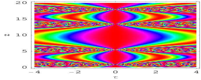
Figure 1: Density plot depicting the nonlinear chirping of the trigonometric solution for $\sigma=0.5$, $\alpha=3.45$, $\lambda=-3.34$, and $\epsilon=-2.78$

4 Nonlinear chirping

In this subsection, we wish to cite an example corresponding to the trigonometric solution, illustrative of the fascinating features of chirping in double-doped fibers, by considering the system in which the GVD and the nonlinearity are distributed according to

$$\beta(z)=\beta_{0}\cos(\sigma z),~{}~{}\gamma(z)=\gamma_{0}\cos(\sigma z),$$ (54)

where $\beta_{0}$, $\gamma_{0}$ and $\sigma(\neq 0)$ are arbitrary constants. In this case, the corresponding gain, and the nonlinear gain of the fiber amplifier are given by

$$g(z)=\frac{\sigma\nu\cos(\sigma z)}{2-2\nu\sin(\sigma z)}-\frac{\mu\lambda m_{0}\cos(\sigma z)}{(1-\nu\sin(\sigma z))^{2}},$$ (55)

$$\chi(z)=\frac{3m_{0}\gamma_{0}}{m^{2}_{0}-2}\cos(\sigma z),$$ (56)

where the parameter $\nu=2c_{0}\beta_{0}/\sigma$ has been introduced for brevity.

Hence the amplitude of the similariton pulse is

$$P(z,\tau)=\frac{\sqrt{(m^{2}_{0}-2)\rho(0)}}{\sqrt{2}(1-\nu{\rm sin}{\sigma}z)}\frac{A+B{\rm cos}^{2}\left[\frac{\tau-\tau_{p}(z)}{W(z)}\right]}{1+D{\rm cos}^{2}\left[\frac{\tau-\tau_{p}(z)}{W(z)}\right]}$$ (57)

where

$$W(z)=\tau_{0}[1-\nu\sin(\sigma z)],$$

and the pulse position $\tau_{p}$ varies with $\tau_{p}=\tau_{c}-(b_{0}\beta_{0}/\sigma)\sin(\sigma z)$. The resultant chirp consisting of linear and nonlinear contributions are derived as [5]

$$\delta\omega(\tau)=\frac{m_{0}}{W(z)}\frac{\tan(\frac{\tau-\tau_{p}}{W(z)})}{1+D\cos^{2}(\frac{\tau-\tau_{p}}{W(z)})}-b_{0}-\frac{2c_{0}\tau_{0}}{W(z)}(\tau-\tau_{p}).~{}~{}$$ (58)

We notice that the first term in Eq. (58) denotes the nonlinear chirp that results from the nonlinear gain, while the last two terms account for the linear chirp. The propagation of this chirped pulse has been depicted in Fig. 1 for various parameter values of $\tau_{0}$ and $\nu=1$.

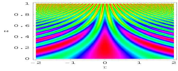
Figure 2: Density plot depicting the nonlinear compression of the trigonometric solution for $\sigma=1.0$, $\alpha=3.45$, $\lambda=-3.34$, and $\epsilon=-2.78$

5 Nonlinear compression

Next, we elucidate the compression problem of the pulse in a dispersion decreasing optical fiber. For the purpose of comparison with Ref. [14, 15], we assume that the GVD and the nonlinearity are distributed according to the following relations

$$\beta(z)=\beta_{0}\exp(-\sigma z),~{}~{}\gamma(z)=\gamma_{0}\exp(\alpha z),$$ (59)

where $\beta_{0}\leq 0$, $\gamma_{0}\geq 0$, and $\sigma\neq 0$. Then from Eq. (34) the expression for gain can be calculated as

$$g(z)=-\alpha+\nu\sigma\frac{e^{-\sigma z}}{1-\nu(1-e^{-\sigma z})}-\frac{\mu\lambda m_{0}\beta_{0}e^{-\sigma z}}{(1-\nu(1-e^{-\sigma z}))^{2}}.$$ (60)

Let us consider the most typical physical situation when the loss in an optical fiber is constant i.e., $\gamma(z)$ is constant. According to Eq. (60), this occurs when $\nu=1$ and $\alpha>0$: $g(z)=-\alpha$, hence the gain is negative. It is remarkable that the width of the solutions presented here tend to zero when $z\rightarrow\infty$.

We apply the above insights to nonlinear compression of the trigonometric solution given by Eq. (46). Then the amplitude of the compressed wave is

$$P(z,\tau)=U(z)\frac{A+B{\rm cos}^{2}\left[\frac{\tau-\tau_{p}(z)}{W(z)}\right]}{1+D{\rm cos}^{2}\left[\frac{\tau-\tau_{p}(z)}{W(z)}\right]},$$ (61)

where

$$U(z)=\frac{\sqrt{(m^{2}_{0}-2)\rho(0){\exp}{[-(\sigma+\alpha)z]}}}{\sqrt{2}[1-\nu(1-{\rm exp}{(-\sigma z)})]}.$$

And $W(z)=\tau_{0}[1-\nu(1-\exp(-\sigma z))].$ Fig. 2 shows that for constant loss the trigonometric pulse can be compressed to any required degree as $z\rightarrow\infty$, while maintaining its respective original shape.

6 Conclusion

In conclusion, for generalized cubic-quintic nonlinear Schrödinger-type equation with variable dispersion, variable Kerr nonlinearity, variable gain or loss, and nonlinear gain, we found exact chirped pulses that can propagate self-similarly subject to simple scaling rules, of this model. The fact that the pulse position of these chirped pulses can be precisely piloted by appropriately tailoring the dispersion profile, is profitably exploited to achieve optimal pulse compression of these newly reported chirped similariton solutions. Studying soliton bistability using the exact solutions found here will be an interesting issue to be pursued. These analytical findings suggest potential applications in areas such as optical fiber compressors, optical fiber amplifiers, nonlinear optical switches, and optical communications.

References

References

- [1] Hasegawa A and Tappert F 1973 Appl. Phys. Lett. 23, 142
- [2] Mollenauer L F, Stolen R H and Gordon J P 1980 Phys. Rev. Lett. 45, 1095
- [3] Agrawal G P Nonlinear Fiber Optics, Academic Press, San Diego, 2001.
- [4] Anderson D, Desaix M, Karlsson M, Lisak M and Quiroga-Teixeiro M L 1993 J. Opt. Soc. Am. B 10, 1185
- [5] Fermann M E, Kruglov V I, Thomsen B C, Dudley J M and Harvey J D 2000 Phys. Rev. Lett. 84, 6010 ; Kruglov V I, Peacock A C, Dudley J M and Harvey J D 2000 Opt. Lett. 25, 1753.
- [6] Kruglov V I, Peacock A C, Harvey J D and Dudley J M 2002 J. Opt. Soc. Am. B 19, 461.
- [7] Limpert J et al 2002 Opt. Express 10, 628.
- [8] Malinowski A et al 2004 Opt. Lett. 29, 2073.
- [9] Peacock A C, Kruhlak R J, Harvey J D and Dudley J M 2002 Opt. Commun. 206, 171.
- [10] Finot C, Millot G, Pitois S, Billet C and Dudley J M 2004 IEEE J. Sel. Top. Quantum Electron. 10, 1211.
- [11] Ilday F Ö, Buckley J R, Clark W G and Wise F W 2004 Phys. Rev. Lett. 92, 213902.
- [12] Moores J D 1996 Opt. Lett. 21, 555.
- [13] Serkin V N and Hasegawa A 2000 Phys. Rev. Lett. 85, 4502.
- [14] Kruglov V I, Peacock A C and Harvey J D 2003 Phys. Rev. Lett. 90, 113902.
- [15] Chen S and Yi L 2005 Phys. Rev. E 71, 016606.
- [16] Chen S, Yi L, Guo D S and Lu P 2005 Phys. Rev. E 71, 016622.
- [17] Méchin D, Im S H, Kruglov V I, Harvey J D 2006 Opt. Lett. 31, 3106.
- [18] Angelis C D 1994 IEEE J. Quant. Electron. 30, 818.
- [19] Abdullaev F K, Gammal A, Tomio L and Frederico T 2001 Phys. Rev. A 63, 043604.
- [20] Xhang W, Wright E M, Pu H and Meystre P 2003 Phys. Rev. A 68, 023605.
- [21] Inouye S et al 1998 Nature (London) 392, 151.
- [22] Serkin V N, Chapela V M, Percino J and Belyaeva T L 2001 Opt. Commun. 192, 237.
- [23] Ndzana F I, Mohamadou A and Kofané T C 2007 Opt. Commun. 275, 421.
- [24] Avelar A T, Bazeia D Cardoso W B 2009 Phys. Rev. E 79, 025602.
- [25] Adib B, Heidari A and Tayyari S F 2009 Commun. Nonlinear Sci. Numer. Simulat. 14, 2034.
- [26] Azzouzi F et al 2008 Chaos, Solitons and Fractals 39, 1304.
- [27] Porsezian K et al 2009 IEEE J. Quntum Electronics 45, 1577.
- [28] Serkin V N, Hasegawa A and Belyaeva T L 2010 Phys. Rev. A 81, 023610.
- [29] Soloman Raju T, Nagaraja Kumar C and Panigrahi P K 2005 J. Phys. A: Math. and Gen. 38, L271.
- [30] Gorza S P, Roig N, Emplit Ph and Haelterman M 2004 Phys. Rev. Lett. 92, 084101 .
- [31] Li Z et al 2002 Phys. Rev. Lett. 89, 263901 .
- [32] Senthilnathan K, Li Q, Nakkeeran K and Wai P K A 2008 Phys. Rev. A 78, 033835.
- [33] Dai C, Wang Y and Yan C 2010 Opt. Commun. 283, 1489.