Multigrid Preconditioner for Nonconforming Discretization of Elliptic Problems with Jump Coefficients

Abstract

In this paper, we present a multigrid preconditioner for solving the linear system arising from the piecewise linear nonconforming Crouzeix-Raviart discretization of second order elliptic problems with jump coefficients. The preconditioner uses the standard conforming subspaces as coarse spaces. Numerical tests show both robustness with respect to the jump in the coefficient and near-optimality with respect to the number of degrees of freedom.

1 Introduction

The purpose of this paper is to present a multigrid preconditioner for solving the linear system arising from the $\mathbb{P}^{1}$ nonconforming Crouzeix-Raviart (CR) discretization of second order elliptic problems with jump coefficients. The multigrid preconditioner we consider here uses pointwise relaxation (point Gauss-Seidel/Jacobi iterative methods) as a smoother, followed by a subspace (coarse grid) correction which uses the standard multilevel structure for the nested $\mathbb{P}_{1}$ conforming finite element spaces. The subspace correction step is motivated by the observation that the standard $\mathbb{P}^{1}$ conforming space is a subspace of the CR finite element space.

One of the main benefits of this algorithm is that it is very easy to implement in practice. The procedure is the same as the standard multigrid algorithm on conforming spaces, and the only difference is the prolongation and restriction matrices on the finest level. Since the spaces are nested, the prolongation matrix is simply the matrix representation of the natural inclusion operator from the conforming space to the CR space.

The idea of using conforming subspaces to construct preconditioners for CR discretization has been used in Xu (1989, 1996) in the context of smooth coefficients. For the case of jumps in the coefficients, domain decomposition preconditioners have been studied in Sarkis (1994b, a) and the BPX preconditioner has been considered in Ayuso de Dios et al. (2010) in connection with preconditioners for discontinuous Galerkin methods.

In the context of jump coefficients, the analysis of multigrid preconditioners for conforming discretizations is given in Xu and Zhu (2008). For CR discretizations, the analysis is more involved due to the nonconformity of the space, and special technical tools developed in Ayuso de Dios et al. (2010) are necessary. Due to space restrictions, we only state the main result (Theorem 3.2 in Section 3), and provide numerical results that support it. Detailed analyses and further discussion of the algorithm will be presented in a forthcoming paper.

The paper is organized as follows. In Section 2, we give basic notation and the finite element discretizations. In Section 3, we present the multigrid algorithm and discuss its implementation and convergence. Finally, in Section 4 we verify numerically the theoretical results by presenting several numerical tests for two and three dimensional model problems.

2 Preliminaries

Let $\Omega\subset\mathbb{R}^{d}$ ($d=2,3$) be an open polygonal domain. Given $f\in L^{2}(\Omega)$, we consider the following model problem: Find $u\in H_{0}^{1}(\Omega)$ such that

$$a(u,v):=(\kappa\nabla u,\nabla v)=(f,v)\quad\forall v\in H_{0}^{1}(\Omega)\,,$$ (1)

where the diffusion coefficient $\kappa\in L^{\infty}(\Omega)$ is assumed to be piecewise constant, namely, $\kappa(x)|_{\Omega_{m}}=\kappa_{m}$ is a constant for each (open) polygonal subdomain $\Omega_{m}$ satisfying $\cup_{m=1}^{M}\overline{\Omega}_{m}=\overline{\Omega}$ and $\Omega_{m}\cap\Omega_{n}=\emptyset$ for $m\neq n$.

We assume that there is an initial (quasi-uniform) triangulation $\mathcal{T}_{0}$, with mesh size $h_{0}$, such that for all $T\in\mathcal{T}_{0}$ $\kappa_{T}:=\kappa(x)|_{T}$ is constant. Let $\mathcal{T}_{j}:=\mathcal{T}_{h_{j}}$ ($j=1,\cdots,J$) be a family of uniform refinement of $\mathcal{T}_{0}$ with mesh size $h_{j}$. Without loss of generality, we assume that the mesh size $h_{j}\simeq 2^{-j}h_{0}\;\;(j=0,\cdots,J)$ and denote $h=h_{J}$.

On each level $j=0,\cdots,J,$ we define $V_{j}$ as the standard $\mathbb{P}^{1}$ conforming finite element space defined on $\mathcal{T}_{j}$. Then the standard conforming finite element discretization of (1) reads:

$$\mbox{Find }u_{j}\in V_{j}\mbox{ such that }a(u_{j},v_{j})=(f,v_{j}),\qquad\forall v_{j}\in V_{j}.$$ (2)

For each $j=0,\cdots,J$, we define the induced operator for (2) as

$$(A_{j}v_{j},w_{j})=a(v_{j},w_{j}),\quad\forall v_{j},w_{j}\in V_{j}.$$

We denote $\mathcal{E}_{h}$ the set of all edges (in 2D) or faces (in 3D) of $\mathcal{T}_{h}$. Let $V^{CR}_{h}$ be the piecewise linear nonconforming Crouzeix-Raviart finite element space defined by:

$$V^{CR}_{h}\!=\!\left\{v\in L^{2}(\Omega)\,:\,v_{|_{T}}\in\,\mathbb{P}^{1}(T)\,\forall T\in\mathcal{T}_{h}\,\mbox{ and }\int_{e}[\![{v}]\!]_{e}ds=0\,\,\forall\,e\in\mathcal{E}_{h}\right\},$$

where $\mathbb{P}^{1}(T)$ denotes the space of linear polynomials on $T$ and $[\![{v}]\!]_{e}$ denotes the jump across the edge/face $e\in\mathcal{E}_{h}$ with $[\![{v}]\!]_{e}=v$ when $e\subset\partial\Omega$. In the sequel, let us denote $V_{J+1}:=V_{h}^{CR}$ for simplicity. We remark that all these finite element spaces are nested, that is,

$$V_{0}\subset\cdots\subset V_{J}\subset V_{J+1}.$$

The $\mathbb{P}^{1}$-nonconforming finite element approximation to (1) reads:

$$\mbox{Find }u\in V^{CR}_{h}:a_{h}(u,w):=\displaystyle\sum_{T\in\mathcal{T}_{J}}\int_{T}\kappa_{T}\nabla u\cdot\nabla w=(f,w),\forall\,w\in V^{CR}_{h}.$$ (3)

The bilinear form $a_{h}(\cdot,\cdot)$ induced a natural energy norm: $|v|_{h,\kappa}:=\sqrt{a_{h}(v,v)}$ for any $v\in V^{CR}_{h}$. In operator form, we are going to solve the linear system

$$Au=f,$$ (4)

where $A$ is the operator induced by (3), namely

$$(Av,w)=a_{h}(v,w),\qquad\forall v,w\in V_{h}^{CR}.$$

3 A Multigrid Preconditioner

The action of the standard multigrid $V$-cycle preconditioner $B:=B_{J+1}:V_{J+1}\mapsto V_{J+1}$ on a given $g\in V_{J+1}$ is recursively defined by the following algorithm (cf. Bramble (1993)):

Algorithm 3.1 ($V$-cycle)

Let $g_{J+1}=g$, and $B_{0}=A_{0}^{-1}.$ For $j=1,\cdots,J+1,$ we define recursively $B_{j}g_{j}$ for any $g_{j}\in V_{j}$ by the following three steps:

1. Pre-smoothing : $w_{1}=R_{j}g_{j};$

2. Subspace correction: $w_{2}=w_{1}+B_{j-1}Q_{j-1}(g_{j}-A_{j}w_{1});$

3. Post-smoothing: $B_{j}g_{j}:=w_{2}+R_{j}^{*}(g_{j}-A_{j}w_{2}).$

In this algorithm, $R_{j}$ corresponds to a Gauss-Seidel or a Jacobi iterative method known as a smoother; and $Q_{j}$ is the standard $L^{2}$ projection on $V_{j}$:

$$(Q_{j}v,w_{j})=(v,w_{j}),\qquad\forall w_{j}\in V_{j},\;\;(j=0,\cdots,J).$$

The implementation of Algorithm 3.1 is almost identical to the implementation of the standard multigrid $V$-cycle (cf. Briggs et al. (2000)). Between the conforming spaces, we use the standard prolongation and restriction matrices (for conforming finite elements). The corresponding matrices between $V_{J}$ and $V_{J+1}$, are however different. The prolongation matrix on $V_{J}$ can be viewed as the matrix representation of the natural inclusion $\mathcal{I}_{J}:V_{J}\to V_{J+1},$ which is defined by

$$(\mathcal{I}_{J}v)(x)=\sum_{e\in\mathcal{E}_{h}}v(m_{e})\psi_{e}(x),$$

where $\psi_{e}$ is the CR basis on the edge/face $e\in\mathcal{E}_{h}$ and $m_{e}$ is the barycenter of $e$. Therefore, the prolongation matrix has the same sparsity pattern as the edge-to-vertex (in 2D), or face-to-vertex (in 3D) connectivity, and each nonzero entry in this matrix equals the constant $1/d$ where $d$ is the space dimension. The restriction matrix is simply the transpose of the prolongation matrix.

The efficiency and robustness of this preconditioner can be analyzed in terms of the effective condition number (cf. Xu and Zhu (2008)) defined as follows:

Definition 1

Let $V$ be a real $N$ dimensional Hilbert space, and $S:V\to V$ be a symmetric positive definition operator with eigenvalues $0<\lambda_{1}\leq\cdots\leq\lambda_{N}.$ The $m$-th effective condition number of $S$ is defined by

$$\mathcal{K}_{m}(S):=\lambda_{N}(S)/\lambda_{m+1}(S).$$

Note that the standard condition number $\mathcal{K}(BA)$ of the preconditioned system $BA$ will be large due to the large jump in the coefficient $\kappa$. However, there might be only a small (fixed) number of small eigenvalues of $BA$, which cause the large condition number; and the other eigenvalues are bounded nearly uniformly. In particular, we have the following main result:

Theorem 3.2

Let $B$ be the multigrid $V$-cycle preconditioner defined in Algorithm 3.1. Then there exists a fixed integer $m_{0}<M,$ depending only on the distribution of the coefficient $\kappa$, such that

$$\mathcal{K}_{m_{0}}(BA)\leq C^{2}|\log h|^{2}=C^{2}J^{2}\;,$$

where the constant $C>0$ is independent of the coefficients and mesh size.

The analysis is based on the subspace correction framework Xu (1992), but some technical tools developed in Ayuso de Dios et al. (2010) are needed to deal with nonconformity of the finite element spaces. Due to space restriction, a detailed analysis will be reported somewhere else.

Thanks to Theorem 3.2 and a standard PCG convergence result (cf. (Axelsson, 1994, Section 13.2)), the PCG algorithm with the multigrid $V$-cycle preconditioner defined in Algorithm 3.1 has the following convergence estimate:

$$|u-u_{i}|_{h,\kappa}\leq 2(\mathcal{K}(BA)-1)^{m_{0}}\left(\frac{CJ-1}{CJ+1}\right)^{i-{m_{0}}}|u-u_{0}|_{h,\kappa}\;,$$

where $u_{0}$ is the initial guess, and $u_{i}$ is the solution of $i$-th PCG iteration. Although the condition number $\mathcal{K}(BA)$ might be large, the convergence rate of the PCG algorithm is asymptotically dominated by $\frac{CJ-1}{CJ+1},$ which is determined by the effective condition number $\mathcal{K}_{m_{0}}(BA)$. Moreover, this bound of asymptotic convergence rate convergence is independent of the coefficient $\kappa$, but depends on the mesh size logarithmically.

4 Numerical Results

In this section, we present several numerical tests in 2D and 3D which verify the result in Theorem 3.2 on the performance of the multigrid $V$-cycle preconditioner described in the previous sections. The numerical tests show that the effective condition numbers of the preconditioned linear systems (with $V$-cycle preconditioner) are nearly uniformly bounded.

4.1 A 2D Example

As a first model problem, we consider equation (1) in the square $\Omega=(-1,1)^{2}$ with coefficient such that, $\kappa(x)=1$ for $x\in\Omega_{1}=(-0.5,0)^{2}\cup(0,0.5)^{2}$, and $\kappa(x)=\epsilon$ for $x$ in the remaining subdomain, $x\in\Omega\setminus\Omega_{1}$ (see Figure 2). By decreasing the value of $\epsilon$ we increase the contrast in the PDE coefficients.

Our initial triangulation on level 0 has mesh size $h_{0}=2^{-1}$ and resolves the interfaces where the coefficients have discontinuities. Then on each level, we uniformly refine the mesh by subdividing each element into four congruent children. In this example, we use 1 forward/backward Gauss-Seidel iteration as pre/post smoother in the multigrid preconditioner, and the stopping criteria of the PCG algorithm is $\|r_{k}\|/\|r_{0}\|<10^{-7}$ where $r_{k}$ is the the residual at $k$-th iteration.

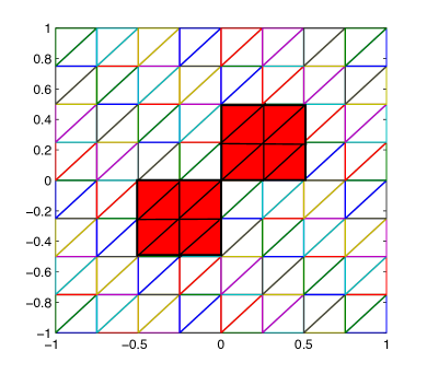
Figure 1: 2D Computational Domain

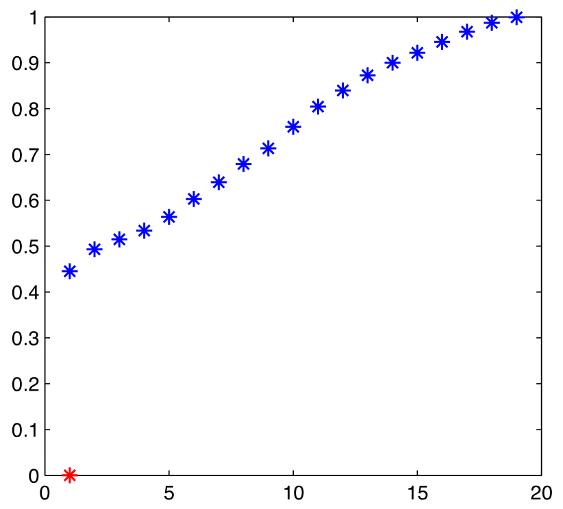
Figure 2: Eigenvalue Distribution of $BA$

Figure 2 shows the eigenvalue distribution of the multigrid $V$-cycle preconditioned system $BA$ when $h=2^{-5}$ (level =4) and $\epsilon=10^{-5}.$ As we can see from this figure, there is only one small eigenvalue that deteriorates with respect to the jump in the coefficient and the mesh size.

Table 1 shows the estimated condition number $\mathcal{K}$ and the effective condition number $\mathcal{K}_{1}$ of $BA$. It can be observed that the condition number $\mathcal{K}$ increases rapidly with respect to the increase of the jump in the coefficients and the number of degrees of freedom. On the other hand, the number of PCG iterations increases only a small amount, and the corresponding effective condition number is nearly uniformly bounded, as predicted by Theorem 3.2.

$\epsilon$	levels	0	1	2	3	4
$1$	$\mathcal{K}$	1.65 (8)	1.83 (10)	1.9 (10)	1.9 (10)	1.89 (10)
	$\mathcal{K}_{1}$	1.44	1.78	1.77	1.78	1.76
$10^{-1}$	$\mathcal{K}$	3.78 (10)	3.69 (11)	3.76 (12)	3.79 (12)	3.88 (12)
	$\mathcal{K}_{1}$	1.89	1.87	1.93	1.92	1.95
$10^{-2}$	$\mathcal{K}$	23.4 (12)	23.6 (13)	24.6 (13)	25.1 (14)	26 (15)
	$\mathcal{K}_{1}$	2.15	1.96	1.99	1.97	2.24
$10^{-3}$	$\mathcal{K}$	218 (13)	223 (14)	232 (15)	238 (16)	246 (16)
	$\mathcal{K}_{1}$	2.19	1.98	2	1.98	2.29
$10^{-4}$	$\mathcal{K}$	2.17e+03 (14)	2.21e+03 (15)	2.31e+03 (16)	2.37e+03 (18)	2.45e+03 (18)
	$\mathcal{K}_{1}$	2.2	1.98	2	1.98	2.3
$10^{-5}$	$\mathcal{K}$	2.17e+04 (15)	2.21e+04 (16)	2.31e+04 (17)	2.37e+04 (19)	2.76e+04 (19)
	$\mathcal{K}_{1}$	2.2	1.98	2	1.98	2.64

Table 1: Estimated condition number $\mathcal{K}$ (number of PCG iterations) and the effective condition number $\mathcal{K}_{1}$

4.2 A 3D Example

In this second example, we consider the model problem (1) in the open unit cube in 3D with a similar setting for the coefficient. We set $\kappa(x)=1$ for $x\in\Omega_{1}=(0.25,0.5)^{3}$ or $x\in\Omega_{2}=(0.5,0.75)^{3}$, and $\kappa(x)=\epsilon$ for the remaining subdomain (that is, for $x\in\Omega\setminus(\Omega_{1}\cup\Omega_{2})$). The domain $\Omega$ and the subdomains just described are shown in Figure 4. The coarsest partition has mesh size $h_{0}=2^{-2}$, and it is set in a way so that it resolves the interfaces where the coefficient has jumps.

To test the effects of the smoother, in this example we used 5 forward/backward Gauss-Seidel as smoother in the multigrid preconditioner. In order to test more severe jumps in the coefficients, we set the stopping criteria $\|r_{k}\|/\|r_{0}\|<10^{-12}$ for the PCG algorithm in this experiment.

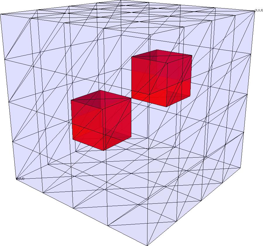
Figure 3: 3D Computational Domain

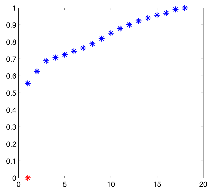
Figure 4: Eigenvalue Distribution of $BA$

Figure 4 shows the eigenvalue distribution of the multigrid $V$-cycle preconditioned system $BA$ when $h=2^{-5}$ (level=3) and $\epsilon=10^{-5}.$ As before, this figure shows that there is only one small eigenvalue that even deteriorates with respect to the jump in the coefficients and the mesh size.

$\epsilon$	levels	0	1	2	3
$1$	$\mathcal{K}$	1.19 (8)	1.34 (11)	1.37 (11)	1.36 (11)
	$\mathcal{K}_{1}$	1.16	1.26	1.31	1.29
$10^{-1}$	$\mathcal{K}$	2.3 (10)	1.94(13)	1.75 (13)	1.67 (14)
	$\mathcal{K}_{1}$	1.60	1.56	1.45	1.43
$10^{-3}$	$\mathcal{K}$	86.01 (11)	63.07 (16)	52.67 (17)	48.19(17)
	$\mathcal{K}_{1}$	2.4	2.12	1.89	1.78
$10^{-5}$	$\mathcal{K}$	8.39+03 (13)	6.15e+03 (18)	5.13e+03 (19)	4.70e+03(19)
	$\mathcal{K}_{1}$	2.44	2.14	1.91	1.80
$10^{-7}$	$\mathcal{K}$	8.39+05 (14)	6.15e+05 (21)	5.13e+05 (23)	4.70e+05(21)
	$\mathcal{K}_{1}$	2.45	2.14	1.91	1.80

Table 2: Estimated condition number $\mathcal{K}$ (number of PCG iterations) and effective condition number $\mathcal{K}_{1}$.

Table 2 shows the estimated condition number $\mathcal{K}$ (with the number of PCG iterations), and the effective condition number $\mathcal{K}_{1}$. As is easily seen from the results in this table, the condition number $\mathcal{K}$ increases when $\epsilon$ decreases, i.e. the condition number grows when the jump in the coefficients becomes larger. On the other hand, the results in Table 2 show that the effective condition number $\mathcal{K}_{1}$ remains nearly uniformly bounded with respect to the mesh size and it is robust with respect to the jump in the coefficient, thus confirming the result stated in Theorem 3.2: a PCG with multigrid $V$-cycle preconditioner provides a robust, nearly optimal solver for the CR approximation to (3).

Acknowledgments

First author has been supported by MEC grant MTM2008-03541 and 2009-SGR-345 from AGAUR-Generalitat de Catalunya. The work of the second and third authors was supported in part by NSF/DMS Awards 0715146 and 0915220, and by DOD/DTRA Award HDTRA-09-1-0036. The work of the fourth author was supported in part by the NSF/DMS Award 0810982.

References

- Axelsson [1994] O. Axelsson. Iterative solution methods. Cambridge University Press, Cambridge, 1994. ISBN 0-521-44524-8.
- Ayuso de Dios et al. [2010] B. Ayuso de Dios, M. Holst, Y. Zhu, and L. Zikatanov. Multilevel Preconditioners for Discontinuous Galerkin Approximations of Elliptic Problems with Jump Coefficients. Arxiv preprint arXiv:1012.1287, 2010.
- Bramble [1993] J. H. Bramble. Multigrid Methods, volume 294 of Pitman Research Notes in Mathematical Sciences. Longman Scientific & Technical, Essex, England, 1993.
- Briggs et al. [2000] W. L. Briggs, V. E. Henson, and S. F. McCormick. A multigrid tutorial. Society for Industrial and Applied Mathematics (SIAM), Philadelphia, PA, second edition, 2000. ISBN 0-89871-462-1.
- Sarkis [1994a] M. Sarkis. Multilevel methods for nonconforming finite elements and discontinuous coefficients in three dimensions. In Domain decomposition methods in scientific and engineering computing (University Park, PA, 1993), volume 180 of Contemp. Math., pages 119–124. Amer. Math. Soc., Providence, RI, 1994a.
- Sarkis [1994b] M. V. Sarkis. Schwarz Preconditioners for Elliptic Problems with Discontinuous Coefficients Using Conforming and Non-Conforming Elements. PhD thesis, Courant Institute of Mathematical Science of New York University, 1994b.
- Xu [1989] J. Xu. Theory of Multilevel Methods. PhD thesis, Cornell University, 1989.
- Xu [1992] J. Xu. Iterative methods by space decomposition and subspace correction. SIAM Review, 34:581–613, 1992.
- Xu [1996] J. Xu. The auxiliary space method and optimal multigrid preconditioning techniques for unstructured meshes. Computing, 56:215–235, 1996.
- Xu and Zhu [2008] J. Xu and Y. Zhu. Uniform convergent multigrid methods for elliptic problems with strongly discontinuous coefficients. Math. Models Methods Appl. Sci., 18(1):77 –105, 2008.