Modeling near-field radiative heat transfer from sharp objects using a general 3d numerical scattering technique

Abstract

We examine the non-equilibrium radiative heat transfer between a plate and finite cylinders and cones, making the first accurate theoretical predictions for the total heat transfer and the spatial heat flux profile for three-dimensional compact objects including corners or tips. We find qualitatively different scaling laws for conical shapes at small separations, and in contrast to a flat/slightly-curved object, a sharp cone exhibits a local minimum in the spatially resolved heat flux directly below the tip. The method we develop, in which a scattering-theory formulation of thermal transfer is combined with a boundary-element method for computing scattering matrices, can be applied to three-dimensional objects of arbitrary shape.

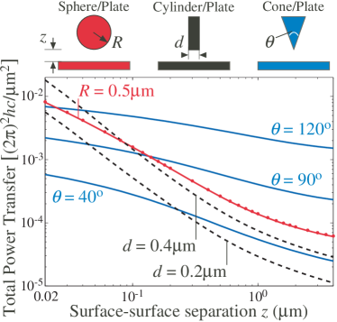
Figure 1: Total thermal transfer between a silica plate and doped silicon objects of various shapes. The plate is semi-infinite, and the objects all have height equal to $1\,\mu\mathrm{m}$ in the $z$-direction. The plate/environment temperature is $T_{P}=300\,\mathrm{K}$ and the objects are at temperature $T_{A}=600\,\mathrm{K}$. Red dots denote results with the sphere scattering matrix determined analytically, the only case in which we have an analytic solution for the scattering matrix.

Introduction: We make the first accurate theoretical predictions for near-field thermal transfer from 3d compact objects of arbitrary shape (including corners or tips) to a dielectric substrate. Our work is motivated by studies of non-contact thermal writing with a hot, sharp object Mamin (1996); Wilder et al. (1998). Theory has predicted Polder and Van Hove (1971); Volokitin and Persson (2001) and experiments have confirmed Shen et al. (2009); Rousseau et al. (2009) that radiative heat transfer between two bodies at different temperatures is greatly enhanced as their separation is reduced to sub-micron scales, due to contributions from evanescent waves. Until the last few years, the only rigorous theoretical results for thermal transfer concerned parallel plates; however, very recently rigorous theoretical predictions for sphere-sphere Narayanaswamy and Chen (2008a) and sphere-plate Krüger et al. (2011a); Otey and Fan (2011) geometries as well as general formalisms for planar structures Bimonte (2009) and arbitrary shapes Messina and Antezza (2011); Krüger et al. (2011a) have been presented. Nevertheless, such techniques were previously implemented only when analytic expressions for the scattering matrices were known (e.g., spheres and plates in 3d). As an alternative, stochastic finite-difference time-domain methods have been used to examine heat transfer for periodic structures Rodriguez et al. (2011), but this method is not computationally well-suited for compact objects in three dimensions. Our technique extends the formalism of Krüger et al. (2011a) directly to arbitrary compact objects. To do this, we use a boundary-element method in which the object is described by a generic surface mesh Rao et al. (1982). We then numerically compute the scattering matrices of this object in a multipole basis; for our study, we employ a cylindrical-wave basis. Unlike the usual spherical-wave basis, this allows us to concentrate our resolution on the surfaces adjacent to the substrate, but requires a new quadrature approach to discretize the scattering matrix. In addition to sphere-plate heat transfer, we study both cylinder-plate and cone-plate configurations (see sketch in Fig. 1), for which no known analytic solution exists. Our results exhibit clear scaling laws for the total heat transfer that distinguish locally flat structures (e.g., cylinders and spheres), from locally sharp structures (cones). In addition, we study the spatial distribution of heat-flux over the substrate, a topic that has been treated previously using a point-dipole approximation for the heat source Mulet et al. (2001). Our results show that the heat flux pattern depends strongly on the shape of the tip. Cones in particular have a flux pattern exhibiting an unusual feature: a local minimum in the heat flux directly below the tip, which we can explain with a modified dipole picture.

Method: In our setup, an object $A$ at (local) temperature $T_{A}$ faces a dielectric plate $P$ at temperature $T_{P}$, in an environment $E$ that is also at temperature $T_{P}$. We use the framework of Rytov’s theory Rytov et al. (1989), in which all sources emit radiation independently. The full non-equilibrium Poynting flux can be computed with radiative sources from $P$ and $E$ only, as the flux from $A$ at temperature $T_{A}$ must equal the flux from $P$ and $E$ at temperature $T_{A}$ (with opposite sign), due to detailed balance Eckhardt (1984). To compute the power flux, we first compute the non-equilibrium electric field correlator $\langle\mathbf{E}(\mathbf{x})\otimes\mathbf{E}^{*}(\mathbf{x}^{\prime})\rangle_{j}$ due to radiation from $j=P,E$ for general $\mathbf{x}\neq\mathbf{x}^{\prime}$ (the Poynting flux will be obtained at the end by taking $\mathrm{lim}_{x^{\prime}\rightarrow x}\nabla_{x^{\prime}}\langle\mathbf{E}\otimes\mathbf{E}^{\prime*}\rangle$) which is expressed as an integral of the general form:

$$\langle\mathbf{E}\otimes\mathbf{E}^{\prime*}\rangle_{j}=\int_{0}^{\infty}\frac{d\omega}{2\pi}\Theta(\omega,T_{j})\langle\mathbf{E}\otimes\mathbf{E}^{\prime*}\rangle_{j,\omega},$$

where $\Theta=\omega^{4}\left(\exp\left(\hbar\omega/k_{B}T\right)-1\right)^{-1}$ Rytov et al. (1989); Eckhardt (1984), $\hbar$ is Planck’s constant and $k_{B}$ the Boltzmann constant. Unless otherwise noted, we consider each frequency $\omega$ separately and drop the $\omega$ subscript below.

The correlator takes on a simple form in an orthogonal basis $\mathbf{E}_{\alpha}(\omega;\mathbf{x})$ for the field degrees of freedom (in our case, these will be cylindrical waves in the $\pm z$ direction), indexed by a (discrete or continuous) index $\alpha$, and represent the correlator as a matrix $\mathbb{D}$. In matrix notation (with implied summation over repeated indices):

$$\langle\mathbf{E}(\mathbf{x})\otimes\mathbf{E}^{*}(\mathbf{x}^{\prime})\rangle=\left(\mathbb{D}\right)_{\alpha^{\prime},\alpha}\mathbf{E}_{\alpha^{\prime}}(\mathbf{x})\otimes\mathbf{E}^{*}_{\alpha}(\mathbf{x}^{\prime}).$$ (1)

$\mathbb{D}=\mathbb{D}_{P}+\mathbb{D}_{E}$ due to statistical independence of the thermal fluctuations, where $\mathbb{D}_{P/E}$ involve sources only from $P$ / $E$. The correlators $\mathbb{D}_{P/E}$ are obtained from the “unperturbed” correlators $\mathbb{D}^{0}_{P/E}$; $\mathbb{D}^{0}_{P}$ involves the plate sources without $A$ and $\mathbb{D}^{0}_{E}$ involves the environment sources with neither $A$ nor $P$ present. The $\mathbb{D}^{0}_{j}$ are known analytically (see below), and the full correlators $\mathbb{D}_{j}$ can be determined from them by use of the Lippmann-Schwinger equation Krüger et al. (2011a); Rahi et al. (2009). In our notation:

$$\mathbb{D}_{j} = \mathbb{O}_{j}\mathbb{D}_{j}^{0}\mathbb{O}_{j}^{\dagger},~{}~{}~{}j=P,E$$ (2)

The $\mathbb{O}_{j}$ are matrices that describe the scattering of incoming and outgoing fields with the allowance for sources in between the objects, described explicitly in Krüger et al. (2011b). These are constructed from the more conventional incoming/outgoing scattering matrices $\mathbb{F}_{P/A}$ Merzbacher (1998); Rahi et al. (2009) for objects $P$ and $A$ individually. As object $P$ is a plate, $\mathbb{F}_{P}$ is known analytically. However, $\mathbb{F}_{A}$ cannot be determined analytically for a general object $A$. Instead, the computation of the scattering matrix elements is accomplished via a boundary-element method Rao et al. (1982), described below. The $z$-component of the Poynting flux at position $\mathbf{x}$, $S_{\mathbf{x}}$, and the total power flux $S_{T}$ through the $z=0$ plane can both be expressed as operator traces: $S_{\mathbf{x}/T}=\operatorname{Re}\mathrm{Tr}\left[\mathbb{S}_{\mathbf{x}/T}\mathbb{D}_{T}\right]$, with $\left(\mathbb{S}_{\mathbf{x}}\right)_{\alpha^{\prime},\alpha}=-\frac{i}{\omega}\hat{\mathbf{z}}\cdot\left[\mathbf{E}_{\alpha}(\mathbf{x})\times\left(\nabla\times\mathbf{E}_{\alpha^{\prime}}(\mathbf{x})\right)^{*}\right]$ and $\left(\mathbb{S}_{T}\right)_{\alpha^{\prime},\alpha}$ given below.

We employ a cylindrical-wave basis of fields $\mathbf{E}_{s,m,k_{\rho},p}(\mathbf{x})$ in which the waves (also known as Bessel beams) propagate in the $\pm z$ direction Tsang et al. (2000). The variable $s=\pm$ refers to the direction of propagation; $m$ is the (integer) angular moment of the field, $0\leq k_{\rho}<\infty$ the radial wavevector, and $p=M,N$ the polarization. The composite index in this case is $\alpha=\{s,m,k_{\rho},p\}$. This basis is especially well-suited to the case considered here in which objects have rotational symmetry about the $z$-axis, as different values of $m$ are decoupled.

To compute the elements of $\mathbb{F}_{A}$, we use a boundary-element method (BEM) Rao et al. (1982); Reid (2010). In this framework, the surface of object $A$ is discretized into a mesh; our numerical method then computes the induced currents from an incident multipole field $\mathbf{E}_{\alpha}(\mathbf{x})$ (here $\alpha=\{s,m,k_{\rho},p\}$). The multipole moments of this current distribution are then computed in a straightforward manner Tsang et al. (2000), which yield the scattering matrix $\mathbb{F}_{A}$ Rahi et al. (2009). Because the cylindrical-wave basis distinguishes between waves in the $\pm z$ direction (unlike a spherical wave basis), and because the near-field thermal transport mostly depends on reflections from adjacent surfaces, we are able to concentrate most of our BEM mesh resolution on the part of the surface of $A$ nearby the plate, greatly improving computational efficiency. For example, in the mesh for a cone below we use $\sim 250$ times more resolution at the tip than at the base.

One complication of cylindrical multipoles is that $k_{\rho}$ is a continuous index and matrix multiplication is turned to integration. For computational purposes, this integration must be approximated as a discrete sum by numerical quadrature. We approximate the integral over $k_{\rho}$ using a Gaussian quadrature scheme Abramowitz and Stegun (1972) for high accuracy. For example, consider the scattering matrix $\mathbb{F}_{A}$ of object $A$; its action on an incident electric field can be discretized as (for simplicity, summation over $m$ and $p$ is suppressed): $\mathbb{F}_{A}\mathbf{E}_{k_{\rho,i}}=\int_{0}^{\infty}\frac{dk_{\rho}^{\prime}}{2\pi}\left(\mathbb{F}_{A}\right)_{k_{\rho}^{\prime};k_{\rho,i}}\mathbf{E}_{k_{\rho}^{\prime}}\approx\sum_{j=0}^{N}w_{j}\left(\mathbb{F}_{A}\right)_{j,i}\mathbf{E}_{k_{\rho,j}}$ where the sets $\{w_{j},k_{\rho,j}\}$ form a set of one-dimensional quadrature weights and points, respectively, and $\left(\mathbb{F}_{A}\right)_{j,i}=\left(\mathbb{F}_{A}\right)_{k_{\rho,j},k_{\rho,i}}$ are the elements of the continuous scattering matrix.

The analytic expression for the non-equilibrium electric field correlator of a plate at temperature $T_{P}$ and environment at $T=0$ expressed in the planewave basis is well-known Rytov et al. (1989); Krüger et al. (2011b). Since there is a standard identity relating planewaves to cylindrical waves, it is a simple exercise to re-express this correlator in the basis of cylindrical multipoles Tsang et al. (2000):

$$\left(\mathbb{D}^{0}_{P}\right)_{\alpha^{\prime},\alpha}=\delta_{\alpha^{\prime},\alpha}\delta_{s,+}\left(\frac{1-\left|r_{k_{\rho},p}\right|^{2}}{4qk_{\rho}}\chi_{p}+\frac{\operatorname{Im}{r_{k_{\rho},p}}}{2|q|k_{\rho}}\chi_{e}\right)$$

Here $r_{k_{\rho},p}$ are the Fresnel coefficients for a dielectric plate, $\chi_{p(e)}=1$ for $k_{\rho}<\omega$ $(k_{\rho}>\omega)$ and zero otherwise, $q=\sqrt{\omega^{2}-k_{\rho}^{2}}$, and $\delta_{i,j}$ is the Kronecker (Dirac) delta function on discrete (continuous) indices; the $\delta_{s,+}$ reflects the fact that only waves propagating in the $+z$ direction are emitted by the plate. The expression for the environment correlator $\mathbb{D}^{0}_{E}$ is given by the same expression as $\mathbb{D}^{0}_{P}$ with $r=0$ and $\delta_{s,+}$ replaced with $\delta_{s,-}$. Finally, the matrix elements for the total power flux are $\left(\mathbb{S}_{T}\right)_{\alpha^{\prime},\alpha}=\frac{2\pi qk_{\rho}}{\omega}\delta_{k_{\rho},k_{\rho}^{\prime}}\delta_{p,p^{\prime}}(-s^{\prime})^{\delta_{p^{\prime},N}}([\chi_{p}-\chi_{e}]s)^{\delta_{p,M}}$.

For the surface meshes, we use approximately 2,500 panels (discretized surface elements) to get $1\%$ convergence, with the panels highly concentrated on the area of the objects nearest to the plate. We retain angular moments up to $|m|=10$, and for each $m$ we perform the $\omega$ and $k_{\rho}$ integrations using 28 and 48 Gaussian quadrature points, respectively. For our study, object $A$ is composed of doped silicon while the substrate $B$ is silica. For the doped silicon dispersion we use a standard Drude-Lorentz model Duraffourg and Andreucci (2006) with a dopant density of $1.4\times 10^{19}\mathrm{cm}^{-3}$, while for silica we use measured optical data Shen et al. (2009).

Results:  Figure 1 shows the geometry-dependence of the total heat transfer rate between different compact objects and a dielectric plate, over surface-surface separations $z$ from several microns down to $20\,\mathrm{nm}$. In addition to the expected near-field enhancement, we observe several crossings as, e.g., the broader surface area of the $R=0.5\,\mu\mathrm{m}$ radius sphere competes with the smaller but flatter surface of the $d=0.4\,\mu\mathrm{m}$ diameter cylinder. For smaller $z$, the ratio of the transfer between the $d=0.4\,\mu\mathrm{m}$ and $d=0.2\,\mu\mathrm{m}$ cylinders approaches the ratio of their surface areas (within $6\%$ at $z=20\,\mathrm{nm}$), as would be expected from a proximity approximation (PA) Narayanaswamy and Chen (2008b); Krüger et al. (2011a). The sphere-plate exhibits the $1/z$ power law as predicted by PA Shen et al. (2009); Rousseau et al. (2009); Krüger et al. (2011a) to within $10\%$ for $z<0.1\,\mu\mathrm{m}$, while the cylinder-plate exhibits agreement to within approximately $10\%$ over this range using a PA based on the integral of the plate-plate heat transfer rate over the cylinder front face and vertical sidewalls. The contribution from the sidewalls can be ignored (leading to a $\sim 1/z^{2}$ transfer rate Volokitin and Persson (2001)) for $z/d\lesssim 0.01$. In contrast to the sphere and cylinders, the cones do not seem to be asymptoting to a power law, and may even have a logarithmic divergence as $z\rightarrow 0$, a fact which we attribute to the scale-invariance of the plate-cone configuration when $z\ll 1\mu\mathrm{m}$ and $z\ll\hbar c/k_{B}T$ (the latter eliminating material dispersion effects). To check the accuracy of our numerical scattering method, we also plot the results for the sphere where $\mathbb{F}_{A}$ is calculated semi-analytically Krüger et al. (2011a), shown as red dots, which agrees to within $1\%$.

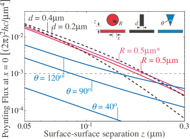
Figure 2: Poynting flux at the origin for the geometries of Fig. 1 with plate/environment temperature $T_{P}=300\,\mathrm{K}$ and object temperature $T_{A}=600\,\mathrm{K}$, using the single-polarization approximation (SPA). The magenta line denotes the sphere-plate without the SPA, and the horizontal dashed line denotes the threshold used for the crossectional flux profiles of Fig. 3.

For thermal writing applications, an important factor to consider is not only the total power delivered to the plate, but also the spatial extent over which this delivery occurs. In order to examine this, we envision a scenario in which a critical magnitude of the $z$-directed Poynting flux is required in order for some change to occur on the plate, for example, the patterning of a thermal mask for later etching Wilder et al. (1998). Figure 2 plots the Poynting flux at $x=0$ as a function of $z$, which will tell us how far away the object must be before it can effect this patterning. The cylinders and spheres converge to the same $\sim 1/z^{2}$ profile for small $z$ (as expected from a PA), whereas the cones all follow $1/z^{2}$ profiles with different coefficients. This $1/z^{2}$ dependence follows from the scale-invariance of the scattering problem for small $z$, combined with the fact that there is a $1/z$ cutoff in the range of $k_{\rho}$ that contributes to the transfer, so that the total number of modes that contribute is proportional to $\int_{0}^{1/z}dk_{\rho}k_{\rho}\sim 1/z^{2}$. In this calculation we have found that the result is dominated by the $N$ polarization ($\mathbf{E}\perp\hat{\mathbf{z}}$), mirroring similar phenomena in other near-field cases Zhang (2007), that results from the behavior of the Fresnel coefficients for high $k_{\rho}$. This is fortunate because we have found that the $M$ contribution to the Poynting flux requires much higher mesh resolution to converge. To check this single-polarization approximation (SPA) for a sphere we also plot the full results, finding that the error from the SPA is $<20\%$ at the largest $z$, decaying to $<10\%$ at smaller $z$; SPA for a cone is discussed below.

Figure 3 plots the Poynting flux as a function of $x$ showing the heat transfer profile. For each object, we chose $z$ to have the same $x=0$ Poynting flux of $10^{-3}(2\pi)^{2}hc/\mu\mathrm{m}^{4}$ (horizontal dashed line in Fig. 2), corresponding to a sphere-plate separation of $\approx 200\,\mathrm{nm}$. The cylinders and $120^{\circ}$ cone all reach this threshold at comparable separations, whereas the $90^{\circ}$ cone is at less than half the separation, and the $40^{\circ}$ cone does not even reach this threshold within the range considered.

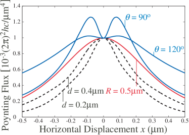
Figure 3: Spatially-resolved heat flux profiles at the substrate surface. $z$ is chosen to fix Poynting flux at $x=0$ at $10^{-3}(2\pi)^{2}hc/\mu\mathrm{m}^{4}$.

Fixing the peak Poynting flux to $10^{-3}(2\pi)^{2}hc/\mu\mathrm{m}^{4}$, in Fig. 3 we plot the Poynting flux profiles for these shapes as a function of $x$. The widths for the cylinders are narrower than the sphere, implying that the cylinders can write higher spatial resolution. Surprisingly, the cones do not exhibit this simple behavior. Rather, the Poynting flux profiles for the two cones are non-monotonic in $x$, with a local minimum at $x=0$. The degree of non-monotonicity appears to increase as the cone becomes sharper.

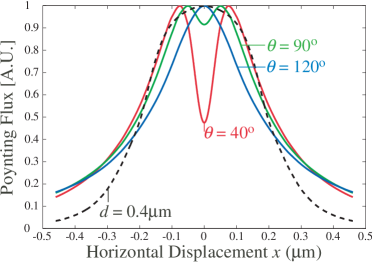
Figure 4: Spatially-resolved heat flux profiles (arbitrary units) at the substrate surface for three cones at a single frequency $\omega=0.3066(2\pi c/\mu\mathrm{m})$ and fixed $z=70\,\mathrm{nm}$. The profiles are normalized so that their maximal value is equal to 1. These profiles are computed without the SPA using much finer meshes. For comparison, the profile for a cylinder of radius $d=400\,\mathrm{nm}$ (using the SPA) is shown as well.

Before attempting to explain this effect, we must first recall that the results of Fig. 2 and Fig. 3 relied on the SPA; although we know this approximation to work well for flat or smoothly curved bodies, it is not obvious that it applies equally well to the cone. To confirm this result without this approximation, we must go to a much denser mesh near the cone tip to ensure mesh convergence; for this, we form a mesh using approximately 12,000 panels for these cones. We have observed that for the shapes and separations of interest here, the Poynting flux profiles at all relevant frequencies have very similar shape, and are simply scaled by a frequency- and material-dependent weight. Therefore, it is sufficient to consider a single frequency, which we pick to be $\omega=0.3066(2\pi c/\mu\mathrm{m})$. The resulting Poynting flux profiles for all three cones at a fixed $z=0.1\,\mu\mathrm{m}$ are shown in Fig. 4; for ease of comparison, all curves are scaled to have a maximum of 1. We also show the $d=0.4\,\mu\mathrm{m}$ cylinder (using the SPA) for comparison. The dip at $x=0$ is less pronounced for the exact curves than for the SPA; in fact, the dip has vanished for $\theta=120^{\circ}$. However, it is still present for $\theta=90^{\circ}$ and is very prominent for $\theta=40^{\circ}$, where the Poynting flux at $x=0$ is less than half of its peak value. Therefore, we conclude that this effect is not a result of our approximations.

We believe the explanation for the dip in the Poynting flux is that as the cone tip becomes sharper, its radiation pattern approaches that of a dipole with axis normal to the plate, which has zero Poynting flux at $x=0$. This explanation predicts that a very thin cylinder with $d\ll z$ should also have a dip in the Poynting flux at $x=0$, which we have also confirmed numerically.

This work was supported by the Army Research Office through the ISN under Contract W911NF-07-D-0004 and by DARPA under Contract No. N66001-09-1-2070-DOD and by DFG grant No. KR 3844/1-1.

References

- Mamin (1996) H. J. Mamin, Appl. Phys. Lett. 69, 433 (1996).
- Wilder et al. (1998) K. Wilder, C. F. Quate, D. Adderton, R. Bernstein, and V. Elings, Appl. Phys. Lett. 73, 2527 (1998).
- Polder and Van Hove (1971) D. Polder and M. Van Hove, Phys. Rev. B 4, 3303 (1971).
- Volokitin and Persson (2001) A. I. Volokitin and B. N. J. Persson, Phys. Rev. B 63, 205404 (2001).
- Shen et al. (2009) S. Shen, A. Narayanaswamy, and G. Chen, Nano Letters 9, 2909 (2009).
- Rousseau et al. (2009) E. Rousseau, A. Siria, G. Jourdan, S. Volz, F. Comin, J. Chevrier, and J.-J. Greffet, Nature Photonics 3, 514 (2009).
- Narayanaswamy and Chen (2008a) A. Narayanaswamy and G. Chen, Phys. Rev. B 77, 075125 (2008a).
- Krüger et al. (2011a) M. Krüger, T. Emig, and M. Kardar, Phys. Rev. Lett. 106, 210404 (2011a).
- Otey and Fan (2011) C. Otey and S. Fan, arXiv 1103.2668 (2011).
- Bimonte (2009) G. Bimonte, Phys. Rev. A 80, 042102 (2009).
- Messina and Antezza (2011) R. Messina and M. Antezza, arXiv 1012.5183 (2011).
- Rodriguez et al. (2011) A. W. Rodriguez, O. Ilic, P. Bermel, I. Celanovic, J. D. Joannopoulos, M. Soljačić, and S. G. Johnson, arXiv 1105.0708 (2011).
- Rao et al. (1982) S. Rao, D. Wilton, and A. Glisson, IEEE Trans. Anten. Prop. 30, 409 (1982).
- Mulet et al. (2001) J. P. Mulet, K. Joulain, R. Carminati, and J. J. Greffet, Appl. Phys. Lett. 78, 2931 (2001).
- Rytov et al. (1989) S. M. Rytov, Y. A. Kravtsov, and V. I. Tatarskii, Principles of Statistical Radiophsics III (Springer-Verlag, 1989).
- Eckhardt (1984) W. Eckhardt, Phys. Rev. A 29, 1991 (1984).
- Rahi et al. (2009) S. J. Rahi, T. Emig, N. Graham, R. L. Jaffe, and M. Kardar, Phys. Rev. D 80, 085021 (2009).
- Krüger et al. (2011b) M. Krüger, T. Emig, G. Bimonte, and M. Kardar, In Preparation (2011b).
- Merzbacher (1998) E. Merzbacher, Quantum Mechanics (John Wiley and Sons, New York, 1998).
- Tsang et al. (2000) L. Tsang, J. A. Kong, and K.-H. Ding, Scattering of Electromagnetic Waves (Wiley, New York, 2000).
- Reid (2010) M. T. H. Reid, Ph.D. thesis, MIT (2010).
- Abramowitz and Stegun (1972) M. Abramowitz and I. A. Stegun, eds., Handbook of Mathematical Functions (Dover, New York, 1972).
- Duraffourg and Andreucci (2006) L. Duraffourg and P. Andreucci, Phys. Lett. A 359, 406 (2006).
- Narayanaswamy and Chen (2008b) A. Narayanaswamy and G. Chen, Phys. Rev. B 77, 075125 (2008b).
- Zhang (2007) Z. M. Zhang, Nano/Microscale heat transfer (McGraw-Hill, 2007).