$\bar{D}^{0}D^{0*}$ $(D^{0}\bar{D}^{0*})$ System in QCD-Improved Many Body Potential

Abstract

For a system of current interest (composed of charm, anticharm quarks and a pair of light ones), we show trends in phenomenological implications of QCD-based improvements to a simple quark model treatment. We employ resonating group method to render this difficult four-body problem manageable. We use a quadratic confinement so as to be able to improve beyond the Born approximation. We report the position of the pole corresponding to $\bar{D}^{0}D^{0*}$ molecule for the best fit of a model parameter to the relevant QCD simulations. We point out the interesting possibility that the pole can be shifted to $3872$ MeV by introducing another parameter $I_{0}$ that changes the strength of the interaction in this one component of $X(3872)$. The revised value of this second parameter can guide future trends in modeling of the full exotic meson $X(3872)$. We also report the changes with $I_{0}$ in the $S$-wave spin averaged cross sections for $\bar{D}^{0}D^{0*}\longrightarrow\omega J/\psi$ and $\bar{D}^{0}D^{0*}\longrightarrow\rho J/\psi$. These cross sections are important regarding the study of QGP (quark gluon plasma).

I Introduction

Considering difficulties in solving quantum chromodynamcis (QCD) for the relevant energies, hadron phenomenology and hadron-hadron scattering is studied mostly through models or effective Lagrangian densities. But as far as possible continuum hadronic models should agree to lattice simulations of QCD and give phenomenological implications having a good comparison with the corresponding hard experimental results. For multiquark systems, a common approach having a fairly good phenomenological record, is the sum of pair-wise interaction model J. Weinstein ; diagrammatic approach ; Gui-Jun Ding Wei Huang Jia-Feng Liu Mu-Lin Yan ; Eric S Swanson ; Y. Cui X-L. Chen ; T. Barnes N. Black ; Wong Swanson Barnes ; Wong Swanson 01 ; Bicudo ; Swanson report 06 ; Wang Huang ; Hiyama prog th physics ; Hiyama physics letter B . The need for improvement in it is indicated even phenomenologically by noting that this model predicts color van der Waals interaction of the inverse-power type between separated hadrons and this has no experimental evidence. At the quark level, good lattice-based improvements B. Masud ; A. M. Green and P. Pennanen ; P. Pennanen ; green2 to this sum of two-body potential model are available which modify it at large distances. These improvements introduced a space dependent form factor $f$ (appearing in eqs. (9), (10) and (11) below) in off-diagonal elements in the overlap, potential and kinetic energy matrices of the model. The additional parameter in $f$ minimizes difference between the two quark two antiquark binding in the improved model to the binding resulting from relevant lattice-generated QCD simulations by UKQCD A.M.Green and C.Michael and M.E.Sainio ; A.M.Green and J. Lukkarinen and P. Pennanen and C.Michael and S.Furui ; A.M.Green and J.Lukkarinen and P. Pennanen and C. Michael ; Petrus Pennanen . The exponential form of $f$ keeps the model agreeing to the pair-wise interaction model in the small distance limit while getting a fairly good agreement to the QCD simulations and solving the van der Waals problem.

It is necessary to find testable implications of these improvements at the meson level in form of multiquark energies (binding) and meson-meson cross-sections. Without these improvements, the $\bar{D}^{0}D^{0*}$ and its coupling to $\omega J/\psi$ or $\rho J/\psi$ has been studied Wong Swanson Barnes ; Wong Swanson 01 ; Cheuk-Yin Wong . Ref. Wong Swanson Barnes ; Wong Swanson 01 report the resulting $\rho J/\psi$ to $\bar{D}^{0}D^{0*}$ cross sections, along with many others. Ref. Cheuk-Yin Wong reports meson-meson potential and eigenvalues for $D\bar{D}^{*}$ and $B\bar{B}^{*}$ four-quark states and find molecular states in the resulting combinations. We are now calculating revised implications for the $\bar{D}^{0}D^{0*}$ system. These implications address some experimental issues of wide interest, for example understanding exotic mesons Godfrey ; Close Vijande 04 ; Shi-Lin Zhu . An important such state is the meson $X(3872)$ which is now generally considered y Dong and a Faessler ; Ortega and Segovia PRD ; Bugg ; Eitchen Lane ; Voloshin 05 ; Lee I W and Faessler A and Gutsche T and Lyubovitskij V E ; Kalashnikova Yu S and Nefediev A V as a mixture of $\bar{D}^{0}D^{0*}$, $D^{+}D^{-*}$ and $c\bar{c}$. Any effort to understand it, thus, should understand quantities depending upon its components. A direct lattice QCD study of it would have to calculate many Wilson loops before arriving at any conclusion. A more manageable route could be to make separate models of its components, find out their consequences and then combine the models to understand $X(3872)$. Our work is the first step in this scheme; we take up $\bar{D}^{0}D^{0*}$ system whose flavor content has an overlap with both isovector $\rho J/\psi$ and isoscalar $\omega J/\psi$ and we study its coupling to both channels.

Ref. Swanson 04 addresses the possibility that $X(3872)$ is a molecular bound state of neutral charm mesons and refs. Braaten a5 ; Braaten a7 ; P. Colangelo and F. De Fazio and S. Nicotri ; Masayasu Harada and Yong-Liang Ma ; T. Mehen and R. Springer assume so. Ref. Eric S Swanson says that $\bar{D}^{0}D^{0*}$ to $\omega J/\psi$ (and $\rho J/\psi$) interaction is needed to understand models of $X(3872)$. $\bar{D}^{0}D^{0*}\longrightarrow\omega(\rho)J/\psi$ scattering is needed to understand the final state interaction in the $X(3872)$ decaying to $J/\psi\rho$ or $J/\psi\omega$ through the intermediate $\bar{D}^{0}D^{0*}$. Refs. Liu Zang Zhu 06 ; Meng Chao 07 describe the role of this final state interaction through the effective lagrangian approach. We present results that may have implications for these final state interactions while being closer to QCD in giving a quark level description. Refs. Braaten and Kusunoki and Nussinov ; Braaten and Kusunoki use the sub-process $\bar{D}^{0}D^{0*}\longrightarrow\bar{D}^{0}D^{0*}$ for the final state interaction in net $B\longrightarrow\bar{D}^{0}D^{0*}K$ process. Our comments also apply to this channel and we have shown below our results for $\bar{D}^{0}D^{0*}\longrightarrow\bar{D}^{0}D^{0*}$ scattering as well. In a recent paper, Braaten and Kang Braaten and Kang say that “in case of $1^{++}$ quantum numbers of $X(3872)$, effects of scattering between $\omega J/\psi$ and charm meson pairs could be significant.” Moreover, $\bar{D}^{0}D^{0*}\longrightarrow\omega(\rho)J/\psi$ scattering is needed for studying the effect of final state interaction between the comovers in relativistic heavy ion collision experiments Barnes in EPJA .

For the $\bar{D}^{0}D^{0*}$ system, another improvement beyond the quark-antiquark pair-wise interaction implemented is ref. Eric S Swanson . This adds a point-wise meson interaction to the coupling resulting from one gluon exchange and calculates the resulting $\bar{D}^{0}D^{0*}$ to $\omega J/\psi$ scattering amplitudes. We, in this paper, present $\bar{D}^{0}D^{0*}$ to $\omega J/\psi$ and $\rho J/\psi$ cross-sections along with an analysis of $\bar{D}^{0}D^{0*}$ binding resulting from the $f$ model A. M. Green and P. Pennanen ; P. Pennanen ; green2 that better fits the available QCD simulations than the one gluon exchange model. In a previous work M. Imran Jamil and Bilal Masud , we used Born approximation to calculate the meson-level consequences of the most developed geometrical form of the $f$ factor. In the present paper, we use a resonating group formalism to avoid the Born approximation used in refs. M. Imran Jamil and Bilal Masud ; T. Barnes E.S. Swanson J. Weinstein ; T. Barnes E.S. Swanson 94 ; T.Barnes NuovoCim for meson-meson scattering and thus report results can be compared with Born approximation Gilani imran bilal faisal . This is essential to be able judge how good is this approximation. To get analytic expressions for the resulting scattering amplitudes, now we use a quadratic confinement and a simpler form of the $f$ factor. We incorporate the spin and flavour dependence. A similar realistic meson-meson treatment for lighter quarks was published earlier masud . We now address a system ($\bar{D}^{0}D^{0*}$) of current interest and give a much more thorough analysis of the meson-meson binding. Moreover, we include the meson-meson cross-sections that are not in masud at all.

These cross sections can be useful in the experimental studies of quark-gluon plasma (QGP) in relativistic heavy ion collisions. One of the promising signature of QGP in heavy ion collision experiments is the suppression of $J/\Psi$ caused by color Debye screening. However the observed suppression may be affected by the interaction of $J/\Psi$ with the comoving Hadrons mainly $\pi$ and $\rho$ Mesons after the hadronization of QGP. The effect of the interaction with the comovers can be significant as the density of these mesons is very high. Thus an estimate of these cross sections can help in identifying any contribution of QGP in observed production rate of $J/\Psi$ in heavy ion collision experiments.

This paper is organized as follows. In Section II we have specified our $q^{2}\bar{q}^{2}$ Hamiltonian and written the spin and flavor wave functions and the form of the position wave function of our system. The section ends with the integral equations for the unknown position factors of our total wave function, as in a resonating group formalism. In Section III, we solve our integral equations for the amplitudes of transition between two channels of our multiquark system. In Section IV we report the best fit values of the parameters used in our formalism along with describing how they are fixed. In Section V, we present our results for the scattering cross-sections and bindings and give conclusion.

II The Hamiltonian Matrix and the Wave Functions

We use the adiabatic approximation to first define the potential for fixed positions of two quarks and two antiquarks. The model we use (of ref. green2 , with position dependence as that of the model $I_{a}$ in ref. P. Pennanen ) improve the kinetic, potential and overlap matrices in the color basis

$$|1\rangle_{c}=|1_{1\bar{3}}1_{2\bar{4}}\rangle_{c},\\ \hskip 18.06749pt|2\rangle_{c}=|1_{1\bar{4}}1_{2\bar{3}}\rangle_{c}.$$ (1)

They fit to the lattice simulations a parameter $k_{f}$ introduced in the off-diagonal position dependent elements of these matrices, while keeping the small distance limit of the model agreeing to the pair-wise model. To avoid Born approximation, we had to use the simplest form

$$f=\text{exp}(-b_{s}k_{f}\sum_{i<j}r_{ij}^{2}).$$ (2)

in the off-diagonal elements that is used in otherwise more developed model version in ref. green2 .

In the next step of the adiabatic approximation, we calculate quark position wave functions. For this, we start by writing our total state vector as a sum over $k$ of product of the gluonic states $|k\rangle_{g}$, known spin and flavor states and the corresponding quark position wave function $\Psi^{k}(\textbf{r}_{1},\textbf{r}_{2},\textbf{r}_{\bar{3}},\textbf{r}_{\bar{4}})$. $|k\rangle_{g}$ is defined as QCD eigenstate that approaches the corresponding colour state $|k\rangle_{c}$ in the small distance limit. The position dependence of the overlaps and potential energy matrices in the $\{|k\rangle_{g}\}$ basis are taken from the above mentioned refs. P. Pennanen ; green2 . For the kinetic energy matrices we use the non-relativistic prescriptions used in ref. B. Masud ; there it is justified through effective hadron Hamiltonian thomas in (space-)lattice QCD. To these we add (after multiplying the appropriate identity matrices) the sum of the corresponding constituent quark masses $m_{i}$ $(i=1,2,\bar{3},\bar{4})$, fixed ES Swanson to meson spectroscopy, to get the total meson-meson Hamiltonian matrix; this semi-relativistic prescription is already used in refs. J. Weinstein ; diagrammatic approach ; B. Masud ; masud . The resulting matrices are improvements to the matrices in basis of eq. (1) of the Hamiltonian appearing in ref. J. Weinstein , i.e.

$$\hat{H}=\sum_{i=1}^{\overline{4}}\Big{[}m_{i}+\frac{\hat{P}_{i}^{2}}{2m_{i}}\Big{]}+\sum_{i<j}v(\textbf{r}_{ij})\mathbf{F}_{i}.\mathbf{F}_{j}.$$ (3)

$\mathbf{F}_{i}$ is the set of color matrices (of $SU(3)_{c}$) for the ith particle. F has $8$ components $F_{a}=\frac{\lambda_{a}}{2}$ for a quark and for an anti quark $F_{a}=-\frac{\lambda_{a}^{*}}{2}$, $a=1,2,3,...,8$. For using our analytic formalism beyond the Born approximation we employed a simple harmonic potential already used in refs. J. Weinstein ; B. Masud ; masud

$$v(\textbf{r}_{ij})=v_{ij}=Cr_{ij}^{2}+\bar{C}\text{ with }i,j=1,2,\bar{3},\bar{4},$$ (4)

rather than more sophisticated forms of refs. Godfrey Isgur 85 ; Cheuk-Yin Wong ; Li Chao . Our neglect of the hyperfine interaction is less serious in $\bar{D}^{0}D^{0*}\rightarrow\omega(\rho)J/\psi$ processes; ref. Eric S Swanson shows that this amplitude is dominated by the confinement interaction.

This specifies our formula of color interactions between different quarks. The explicit color dependent factor in it is $\mathbf{F}_{i}.\mathbf{F}_{j}$ and that is flavor independent in consistent with the color charge on a quark on any flavor being same. Its quadratic confining coefficient $Cr_{ij}^{2}+\bar{C}$ is to replace the more sophisticated forms of refs. Godfrey Isgur 85 ; Cheuk-Yin Wong ; Li Chao in which the coefficient of the confining term, the QCD string tension, is everywhere taken to be flavor independent; the string tension models the energy density of the gluonic field originating from color charges and color charges are same for each flavor. The confining term we use is the $Cr_{ij}^{2}$ and its coefficient $C$ is accordingly taken to be flavor independent. This gluonic field energy density is calculated in the lattice QCD simulations of ref. Fumiko Okiharu and this work advocates a flavor independent string tension. The constant term $\bar{C}$ is added to the flavor dependent sum of constituent quark masses in our actual formulas for meson masses, for example in eq. (43) below.

As in the resonating group method, we factorize $\Psi^{k}$ into known and unknown factors to utilize the well known SHO position wave functions $\xi_{k}(\textbf{y}_{k})$ and $\zeta_{k}(\textbf{z}_{k})$ within each quark antiquark subsystem

$$|\Psi(\textbf{r}_{1},\textbf{r}_{2},\textbf{r}_{\bar{3}},\textbf{r}_{\bar{4}};g)\rangle=\sum_{k=1}^{2}|k\rangle_{g}|k\rangle_{f}|k\rangle_{s}\Psi_{c}(\textbf{R}_{c})\chi_{k}(\textbf{R}_{k})\xi_{k}(\textbf{y}_{k})\zeta_{k}(\textbf{z}_{k}).$$ (5)

Where $|k\rangle_{f}$ are the flavor states and $|k\rangle_{s}$ are the spin states. Here $\textbf{R}_{c}$ is the c.m. position vector. The inter-cluster vector $\textbf{R}_{k}$ and in-cluster vectors $\textbf{y}_{k}$ and $\textbf{z}_{k}$ are shown in figs. 1 and 2, which also define the topologies $k=1,2$. For example,

$$\textbf{R}_{1}=\frac{(\textbf{r}_{1}+r\textbf{r}_{\overline{3}}-r\textbf{r}_{2}-\textbf{r}_{\overline{4}})}{(1+r)}.$$ (6)

Here $r=\frac{m_{c}}{m}$, with $m,m_{c}$ being the constituent mass of light (up or down) and charm quarks respectively.

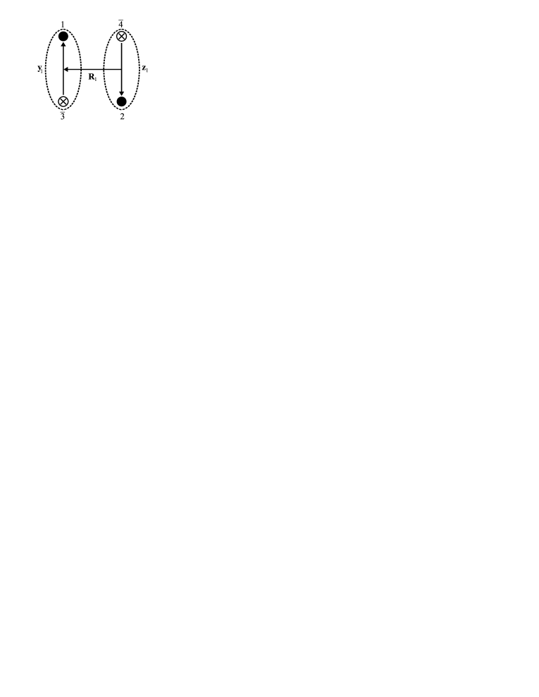
Figure 1: Topology 1.

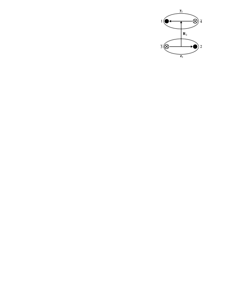
Figure 2: Topology 2

The sizes $d_{k1}$ and $d_{k2}$ of the known quark antiquark clusters are also parameters of our model. $d_{k1}$ is defined by

$$\xi_{k}(\textbf{y}_{k})=\frac{1}{(2\pi d_{k1}^{2})^{\frac{3}{4}}}\text{exp}\Big{(}\frac{-\textbf{y}_{k}^{2}}{4d_{k1}^{2}}\Big{)}.$$ (7)

$d_{k2}$ replaces $d_{k1}$ in $\zeta_{k}(\textbf{z}_{k})$. The unknown inter-cluster factor $\chi_{k}(\textbf{R}_{k})$ is our variational function found by solving integral eq. (8) for it. To get this equation, we set the overlap of an arbitrary variation $|\delta\Psi\rangle$, in $|\Psi\rangle$ of eq. (5), with $(\hat{H}-E_{c})|\Psi\rangle$ as zero and reading off the coefficients of the arbitrary variations $\chi_{k}(\textbf{R}_{k})$ with $k=1,2$. This gives

$$\sum_{l=1}^{2}\int d^{3}\textbf{y}_{k}d^{3}\textbf{z}_{k}\hskip 3.61371pt{}_{f}\langle k|l\rangle_{f}\hskip 3.61371pt{}_{s}\langle k|l\rangle_{s}\hskip 3.61371pt\xi_{k}(\textbf{y}_{k})\zeta_{{k}}(\textbf{z}_{k})_{g}\langle k|\hat{H}-E_{c}|\l\rangle_{g}\chi_{l}(\textbf{R}_{l})\xi_{l}(\textbf{y}_{l})\zeta_{l}(\textbf{z}_{l})=0.$$ (8)

The trivial integration over the c.m. position $\textbf{R}_{c}$ could be performed to give a finite result (implied in above equation) using, say, a box normalization. It is to be noted that our total meson-meson Hamiltonian is an identity operator in the flavor and spin basis because it differs from that in eq. (3) only through the position dependent $f$ and we are neglecting the spin-spin hyperfine interaction.

We use ${}_{g}\langle k|\l\rangle_{g}$, ${}_{g}\langle k|\hat{V}|\l\rangle_{g}$ and ${}_{g}\langle k|\hat{K}|\l\rangle_{g}$ of refs. green2 ; B. Masud to get ${}_{g}\langle k|\hat{H}-E_{c}|\l\rangle_{g}$ required in eq. (8). These form the matrices:

$$N\equiv\{N_{kl}\}\equiv\{_{g}\langle k\mid l\rangle_{g}\}=\left(\begin{array}[]{cc}1&\frac{1}{3}f\\ \frac{1}{3}f&1\\ \end{array}\right),$$ (9)

$$V\equiv\{V_{kl}\}\equiv\{_{g}\langle k\mid\hat{V}\mid l\rangle_{g}\}~{}~{}~{}~{}~{}~{}~{}~{}~{}~{}~{}~{}~{}~{}~{}~{}~{}~{}~{}~{}~{}~{}~{}~{}~{}~{}~{}~{}~{}~{}~{}~{}~{}~{}~{}~{}~{}~{}~{}~{}~{}~{}~{}~{}~{}~{}~{}~{}~{}~{}~{}~{}~{}~{}~{}~{}~{}~{}~{}~{}~{}~{}~{}~{}~{}~{}~{}~{}~{}~{}~{}~{}~{}~{}~{}~{}~{}~{}~{}~{}~{}~{}$$

$$=\left(\begin{array}[]{cc}-\frac{4}{3}(v_{1\overline{3}}+v_{2\overline{4}})&\frac{4}{9}f(v_{12}+v_{\overline{3}\overline{4}}-v_{1\overline{3}}-v_{2\overline{4}}-v_{1\overline{4}}-v_{2\overline{3}})\\ \frac{4}{9}f(v_{12}+v_{\overline{3}\overline{4}}-v_{1\overline{3}}-v_{2\overline{4}}-v_{1\overline{4}}-v_{2\overline{3}})&-\frac{4}{3}(v_{1\overline{4}}+v_{2\overline{3}})\end{array}\right)$$ (10)

$$K\equiv\{K_{kl}\}\equiv{}_{g}\langle k|\hat{K}|\ l\rangle_{g}=N(f)_{k,l}^{\frac{1}{2}}\Big{(}\sum_{i=1}^{\overline{4}}-\frac{\nabla_{i}^{2}}{2m}\Big{)}N(f)_{k,l}^{\frac{1}{2}}.$$ (11)

For $\bar{D}^{0}D^{0*}$ (chosen as channel 1 with $k=1$), the total spin is 1. Angular momentum conservation tells that in the quark exchanged channels ($\omega J/\psi$ and $\rho J/\psi$ corresponding to $k=2$ the total spin should be 1. These spin states are denoted by

$$|1\rangle_{s}=|P_{1\overline{3}}V_{2\overline{4}}\rangle$$ (12)

$$|2\rangle_{s}=|V_{1\overline{4}}V_{2\overline{3}}\rangle,$$ (13)

where $P$ represents a pseudo-scalar and $V$ represents a vector meson. We utilized the rotational symmetry of our problem to write each of these S=1 states as $\frac{1}{\sqrt{3}}\left(|1,1\rangle+|1,0\rangle+|1,-1\rangle\right)$ with the second label as the $S_{z}$ quantum number. We then used the completeness of the meson and then quark spins, along with the required Clebsch-Gordan coefficients, to arrive at the following for ${}_{s}\langle k|l\rangle_{s}$ in eq.(8)

$${}_{s}\langle 1|2\rangle_{s}=_{s}\langle 2|1\rangle_{s}=\frac{1}{\sqrt{2}}.$$ (14)

The flavor content of our channel-1 is unique

$$|1\rangle_{f}=|\bar{c}u\rangle|c\bar{u}\rangle.$$ (15)

For the second channel, it depends on our choice of mesons in it:

$$|2\rangle_{f}=\left(\begin{array}[]{c}\frac{1}{\sqrt{2}}|u\bar{u}+d\bar{d}\rangle|c\bar{c}\rangle~{}~{}~{}~{}\text{for}~{}~{}~{}~{}~{}\omega J/\psi~{}~{}~{}\text{mesons}\\ \frac{1}{\sqrt{2}}|u\bar{u}-d\bar{d}\rangle|c\bar{c}\rangle~{}~{}~{}~{}\text{for}~{}~{}~{}~{}~{}\rho J/\psi~{}~{}~{}~{}\text{mesons}\\ \end{array}\right).$$ (16)

This gives in eq.(8)

$${}_{f}\langle 1|2\rangle_{f}=\frac{1}{\sqrt{2}}$$ (17)

for both $\omega J/\psi$ and $\rho J/\psi$ in channel 2.

III Solving The Integral Equations

When eqs. (9)-(11) and eqs. (14), (17) are substituted in eq. (8), we get the following equation

$$\int d^{3}\textbf{R}_{k}^{\prime}\Big{[}\textbf{K}_{kk}(\textbf{R}_{k},\textbf{R}_{k}^{\prime})+\textbf{V}_{kk}(\textbf{R}_{k},\textbf{R}_{k}^{\prime})+(\sum_{i=1}^{\overline{4}}m_{i}-E_{c})\textbf{N}_{kk}(\textbf{R}_{k},\textbf{R}_{k}^{\prime})\Big{]}\chi_{k}(\textbf{R}_{k}^{\prime})+~{}~{}~{}~{}$$

$$\int_{l\neq k}d^{3}\textbf{R}_{l}\Big{[}\textbf{K}_{kl}(\textbf{R}_{k},\textbf{R}_{l})+\textbf{V}_{kl}(\textbf{R}_{k},\textbf{R}_{l})+(\sum_{i=1}^{\overline{4}}m_{i}-E_{c})\textbf{N}_{kl}(\textbf{R}_{k},\textbf{R}_{l})\Big{]}\chi_{l}(\textbf{R}_{l})=0,~{}~{}~{}~{}~{}~{}$$ (18)

with the kernels $\textbf{K}_{kl}(\textbf{R}_{k},\textbf{R}_{l}^{\prime})$, $\textbf{V}_{kl}(\textbf{R}_{k},\textbf{R}_{l}^{\prime})$ and $\textbf{N}_{kl}(\textbf{R}_{k},\textbf{R}_{l}^{\prime})$ defined, in the notation of eq. (8), by

$$\int d^{3}\textbf{y}_{k}d^{3}\textbf{z}_{k}\xi_{k}(\textbf{y}_{k})\zeta_{{k}}(\textbf{z}_{k})K_{kl}\hskip 1.4457pt\chi_{l}(\textbf{R}_{l})\xi_{l}(\textbf{y}_{l})\zeta_{l}(\textbf{z}_{l})=\frac{2}{\delta_{kl}+1}\int d^{3}\textbf{R}_{l}^{\prime}\textbf{K}_{kl}(\textbf{R}_{k},\textbf{R}_{l}^{\prime})\chi_{l}(\textbf{R}_{l}^{\prime})~{}~{}~{}~{}~{}$$ (19)

$$\int d^{3}\textbf{y}_{k}d^{3}\textbf{z}_{k}\xi_{k}(\textbf{y}_{k})\zeta_{{k}}(\textbf{z}_{k})V_{kl}\hskip 1.4457pt\chi_{l}(\textbf{R}_{l})\xi_{l}(\textbf{y}_{l})\zeta_{l}(\textbf{z}_{l})=\frac{2}{\delta_{kl}+1}\int d^{3}\textbf{R}_{l}^{\prime}\textbf{V}_{kl}(\textbf{R}_{k},\textbf{R}_{l}^{\prime})\chi_{l}(\textbf{R}_{l}^{\prime})~{}~{}~{}~{}$$ (20)

$$\int d^{3}\textbf{y}_{k}d^{3}\textbf{z}_{k}\xi_{k}(\textbf{y}_{k})\zeta_{{k}}(\textbf{z}_{k})N_{kl}\hskip 1.4457pt\chi_{l}(\textbf{R}_{l})\xi_{l}(\textbf{y}_{l})\zeta_{l}(\textbf{z}_{l})=\frac{2}{\delta_{kl}+1}\int d^{3}\textbf{R}_{l}^{\prime}\textbf{N}_{kl}(\textbf{R}_{k},\textbf{R}_{l}^{\prime})\chi_{l}(\textbf{R}_{l}^{\prime}).~{}~{}~{}~{}$$ (21)

The factor $\frac{2}{\delta_{kl}+1}$ takes care of the off-diagonal spin and flavor overlap factors both $=\frac{1}{\sqrt{2}}$. The spatial integrations on the left hand side of eqs. (19-21) and resulting kinetic energy, interaction and normalization kernels are reported in Appendix A. A comparison of kernels themselves can have a dynamical result; ref. Masutani tells that if the interaction kernel is proportional to the normalization kernel, the interaction does not contribute to the interaction between mesons. Eqs. (49) and (55) in the Appendix A show that such is the case in our calculations for a single channel completely described by the diagonal terms in kernels in these equations. For quadratic confinement in one channel approximation ref. Masutani also gets the same result for the interaction between the mesons. But with an improved model for two channel meson-meson interaction our full results are obtained by substituting diagonal as well as off-diagonal terms in eq. (18) and in our case the interaction kernel is not proportional to the normal kernel and hence the quadratic confinement contributes to the interaction between mesons. This is a non-trivial result that can be compared with the baryon-baryon interaction where refs. OkaYazaki 1981 ; Burger report the quark-exchange kernel generated by purely quadratic confinement being proportional to the norm kernel and thus in this case the quadratic confinement does not contribute to (the baryon baryon) interaction. If confinement contributes to the meson-meson interaction, it may worsen the van der Walls force problem between isolated mesons that results by a sum of two-body potential but is against the empirical evidence. But, as mentioned in the introduction, we are finding meson level dynamical implications of the quark potential model improvements P. Pennanen ; green2 ; A. M. Green and P. Pennanen that use multi-quark interactions in form of the $f$ factor to avoid this problem; many works, including ref. OkaYazaki closely related to OkaYazaki 1981 , had earlier suggested that many body interaction is needed to avoid this long range interaction between mesons.

Using all the kernels, we get two integral equations for $k=1,2$; we write here one of them:

$$\Big{[}\frac{3}{4}(\omega_{21}+\omega_{22})-\frac{s_{2}}{2m}\underline{\nabla}_{\textbf{R}_{2}}^{2}-\frac{8}{3}\bar{C}-4C[d_{21}^{2}+d_{22}^{2}]+2m(r+1)-E_{c}\Big{]}\chi_{2}(\textbf{R}_{2})$$

$$+l_{0}\int d^{3}\textbf{R}_{1}\Bigg{[}-\frac{1}{2m}\frac{1}{6}\Big{[}r_{21}\textbf{R}_{1}^{2}+r_{22}\textbf{R}_{2}^{2}+r_{20}\Big{]}+\frac{1}{2}\Big{[}n_{1}\textbf{R}_{1}^{2}+n_{0}\Big{]}$$

$$-\frac{1}{6}\Big{(}E_{c}+\frac{8}{3}\bar{C}-2m(r+1)\Big{)}\Bigg{]}\text{exp}(-l_{1}\textbf{R}_{1}^{2}-l_{2}\textbf{R}_{2}^{2})\chi_{1}(\textbf{R}_{1})=0.$$ (22)

Here $s_{2}$, $\omega^{,}s$, $l^{,}s$, $n^{,}s$ and $r^{,}s$ depend upon the constituent quark masses, sizes of mesons the parameter $k_{f}$ and $b_{s}$; see Appendix A. It is clear from this equation that off-diagonal parts vanish for large values of $\textbf{R}_{1}$ and $\textbf{R}_{2}$. With no interaction in this limit between the two mesons, the total center of mass energy in the large separation limit will be the sum of kinetic energies of the relative motion of mesons and masses of the two mesons. This gives an alternative mesonic form for the diagonal terms survived in the large distance (no interaction limit), which can be utilized to write our integral equations as

$$\Big{[}M_{x}+M_{J/\psi}-\frac{1}{2\mu_{xJ/\psi}}\underline{\nabla}_{\textbf{R}_{2}}^{2}-E_{c}\Big{]}\chi_{2}(\textbf{R}_{2})+l_{0}\int d^{3}\textbf{R}_{1}\Bigg{[}-\frac{1}{2m}\frac{1}{6}\Big{[}r_{21}\textbf{R}_{1}^{2}+r_{22}\textbf{R}_{2}^{2}+r_{20}\Big{]}$$

$$+\frac{1}{2}\Big{[}n_{1}\textbf{R}_{1}^{2}+n_{0}\Big{]}-\frac{1}{6}\Big{(}E_{c}+\frac{8}{3}\bar{C}-2m(r+1)\Big{)}\Bigg{]}\text{exp}(-l_{1}\textbf{R}_{1}^{2}-l_{2}\textbf{R}_{2}^{2})\chi_{1}(\textbf{R}_{1})=0,\hskip 28.45274pt$$ (23)

with $x=\omega,\rho$, and a similar one with the diagonal term as $\Bigg{[}M_{D}+M_{\bar{D}^{0*}}-\frac{1}{2\mu_{\bar{D}^{0}\bar{D}^{0*}}}\underline{\nabla}_{\textbf{R}_{1}}^{2}-E_{c}\Bigg{]}$. By taking Fourier transform of eq. (23), we get

$$\Big{[}M_{x}+M_{J/\psi}+\frac{1}{2\mu_{xJ/\psi}}\textbf{P}_{2}^{2}-E_{c}\Big{]}\chi_{2}(\textbf{P}_{2})-\frac{1}{2m}\frac{r_{22}}{6}A_{1}(l_{1})F_{b}(\textbf{P}_{2},l_{2})$$

$$+\Big{[}\Big{(}-\frac{1}{2m}\frac{r_{20}}{6}+\frac{n_{0}}{2}-\frac{E_{c}^{\prime}}{6}\Big{)}A_{1}(l_{1})+\Big{(}-\frac{1}{2m}\frac{r_{21}}{6}+\frac{n_{1}}{2}\Big{)}B_{1}(l_{1})\Big{]}F_{a}(\textbf{P}_{2},l_{2})=0.\hskip 28.45274pt$$ (24)

where, $E_{c}^{\prime}=E_{c}+\frac{8}{3}\bar{C}-2m(r+1).$ In these equations

$$A_{k}(u)=l_{0}\int d^{3}\textbf{R}_{k}\text{exp}[-u\textbf{R}_{k}^{2}]\chi_{k}(\textbf{R}_{k})$$ (25)

$$B_{k}(u)=l_{0}\int d^{3}\textbf{R}_{k}\text{exp}[-u\textbf{R}_{k}^{2}]\textbf{R}_{k}^{2}\chi_{k}(\textbf{R}_{k})$$ (26)

$$F_{a}(\textbf{P}_{k},u)\equiv\int\frac{d^{3}\textbf{R}_{k}}{(2\pi)^{\frac{3}{2}}}\text{exp}[i\textbf{P}_{k}.\textbf{R}_{k}]\text{exp}[-u\textbf{R}_{k}^{2}]=\frac{1}{(2u)^{\frac{3}{2}}}\text{exp}\Bigg{[}-\frac{\textbf{P}_{k}^{2}}{4u}\Bigg{]}$$ (27)

$$F_{b}(\textbf{P}_{k},u)\equiv\int\frac{d^{3}\textbf{R}_{k}}{(2\pi)^{\frac{3}{2}}}\text{exp}[i\textbf{P}_{k}.\textbf{R}_{k}]\textbf{R}_{k}^{2}\text{exp}[-u\textbf{R}_{k}^{2}]=F_{a}(\textbf{P}_{k},u)\Bigg{[}\frac{1}{2u}\Bigg{]}\Bigg{[}3-\frac{\textbf{P}_{k}^{2}}{2u}\Bigg{]}.\hskip 36.135pt$$ (28)

For the incoming waves in the first channel, our two integral equations (eq. (24) and the other one; we now write both) can be formally solved B. Masud as (see appendix-B for details)

$$\chi_{1}(p_{1})=\frac{\delta(p_{1}-p_{c}(1))}{p_{c}^{2}(1)}-\frac{1}{\Delta_{1}(p_{1})}\Big{[}W_{1}^{(1)}A_{2}(l_{2})+W_{2}^{(1)}B_{2}(l_{2})\Big{]}\hskip 36.135pt$$ (29)

$$\chi_{2}(p_{2})=-\frac{1}{\Delta_{2}(p_{2})}\Big{[}W_{1}^{(2)}A_{1}(l_{1})+W_{2}^{(2)}B_{1}(l_{1})\Big{]}.$$ (30)

Here

$$\Delta_{1}(p_{1})=\frac{p_{1}^{2}}{2\mu_{D^{0}\bar{D}^{0*}}}+M_{D^{0}}+M_{\bar{D}^{0*}}-E_{c}-i\epsilon\texttt{ }$$ (31)

for an infinitesimal $\epsilon$. Similarly,

$$\Delta_{2}(p_{2})=\frac{p_{2}^{2}}{2\mu_{xJ/\psi}}+M_{x}+M_{J/\psi}-E_{c}-i\epsilon\texttt{ }$$ (32)

$$p_{c}(1)=\sqrt{2\mu_{D^{0}\bar{D}^{0*}}(E_{c}-M_{D^{0}}-M_{\bar{D}^{0*}})}\hskip 36.135pt$$ (33)

$$p_{c}(2)=\sqrt{2\mu_{xJ/\psi}(E_{c}-M_{x}-M_{J/\psi})}.$$ (34)

$$W_{1}^{(1)}=\Big{[}-\frac{1}{2m}\frac{r_{11}}{6}+\frac{n_{1}}{2}\Big{]}F_{b}(p_{c}(1),l_{1})+\Big{[}-\frac{1}{2m}\frac{r_{10}}{6}+\frac{n_{0}}{2}-\frac{E_{c}^{\prime}}{6}\Big{]}F_{a}(p_{c}(1),l_{1})$$ (35)

$$W_{2}^{(1)}=-\frac{1}{2m}\frac{r_{12}}{6}F_{a}(p_{c}(1),l_{1})$$ (36)

$$W_{1}^{(2)}=-\frac{1}{2m}\frac{r_{22}}{6}F_{b}(p_{c}(2),l_{2})+\Big{[}-\frac{1}{2m}\frac{r_{20}}{6}+\frac{n_{0}}{2}-\frac{E_{c}^{\prime}}{6}\Big{]}F_{a}(p_{c}(2),l_{2})\hskip 36.135pt$$ (37)

$$W_{2}^{(2)}=\Big{[}-\frac{1}{2m}\frac{r_{21}}{6}+\frac{n_{1}}{2}\Big{]}F_{a}(p_{c}(2),l_{2}).$$ (38)

From eqs. (29) and (30) we can read off the T-matrix elements $T_{11}$ and $T_{21}$ B. Masud as co-efficient of Green’s function operators $-\frac{1}{\Delta_{1}(p_{1})}$ and $-\frac{1}{\Delta_{2}(p_{2})}$ respectively. So, we have

$$T_{11}=2\mu_{D^{0}\bar{D}^{0*}}\frac{\pi}{2}p_{c}(1)\Big{[}W_{1}^{(1)}A_{2}(l_{2})+W_{2}^{(1)}B_{2}(l_{2})\Big{]}$$ (39)

$$T_{21}=2\mu_{xJ\psi}\frac{\pi}{2}p_{c}(1)\sqrt{\frac{v_{2}}{v_{1}}}\Big{[}W_{1}^{(2)}A_{1}(l_{1})+W_{2}^{(2)}B_{1}(l_{1})\Big{]},$$ (40)

where $v_{1}=p_{c}(1)/\mu_{D^{0}\bar{D}^{0*}}~{}\text{and}~{}v_{2}=p_{c}(2)/\mu_{xJ\psi}\texttt{ }.$ Similarly $T_{22}$ and $T_{12}$ can be found for the incoming waves in the 2nd channel, with the $V_{2}$ in Appendix-B accordingly changed. These are

$$T_{22}=2\mu_{xJ\psi}\frac{\pi}{2}p_{c}(2)\Big{[}W_{1}^{(2)}A_{1}(l_{1})+W_{2}^{(2)}B_{1}(l_{1})\Big{]}$$ (41)

$$T_{12}=2\mu_{D^{0}\bar{D}^{0*}}\frac{\pi}{2}p_{c}(2)\sqrt{\frac{v_{1}}{v_{2}}}\Big{[}W_{1}^{(1)}A_{2}(l_{2})+W_{2}^{(1)}B_{2}(l_{2})\Big{]}.$$ (42)

IV Parameters fixing

At the quark level we adopt the model of refs. P. Pennanen ; green2 that includes the parameters $k_{f}$ and $b_{s}$ in the gluonic field overlap factor $f$. We take the value of $k_{f}=0.075$ green2 and $b_{s}$ as $0.18$ Ge$V^{2}$ Fumiko Okiharu . Our own contribution is in using the meson wave functions to find the hadron level implications for our chosen channels. These are eigenfunctions of potential of eq. (4) which has parameters $C$ and $\bar{C}$ whose numerical values we find by equating relevant terms in the large distance limit of eq. (22) to the $J/\psi$ meson mass; see eq. (23). This gives

$$M_{J/\psi}=\frac{3}{4}\omega_{22}-\frac{4}{3}\bar{C}-4Cd_{22}^{2}+2m_{c}.$$ (43)

Comparing eqs. (10) and (4) with the standard form of potential of a simple harmonic oscillator gives $-4C/3=\mu_{c\bar{c}}\omega_{22}^{2}/2$. Using this and $\omega_{22}=1/m_{c}d_{22}^{2}$, we can eliminate $C$ and the size $d_{22}$ in favor of $\omega_{22}$ to get

$$M_{J/\psi}=\frac{3}{2}\omega_{22}-\frac{4}{3}\bar{C}+2m_{c}.$$ (44)

It is to be noted that this equation tells that in our model the dynamics of quarks, incorporating the effects of the glounic field in the form of potential, causes the mass of the quark antiquark cluster (a meson) to be a few percent different to the mere sum $2m_{c}$ of quark masses. Our choice in eq. (4) of using a simple harmonic oscillator potential with a known total energy allows us to write kinetic energy as known total energy minus potential energy. Thus the origin of clustering, or charm-anticharm quarks binding, is in the parameters $C$ and $\bar{C}$ of the potential in eq. (4). The factor $-\frac{4}{3}$ in eq. (44) multiplying $\bar{C}$ is a color factor which is the color expectation value of the $\mathbf{F}_{i}.\mathbf{F}_{j}$ operator in eq. (3) and we have defined $C$ by $-4C/3=\mu_{c\bar{c}}\omega_{22}^{2}/2$ with positive $\omega_{22}$, making $C$ to be negative. Below we replace $C$ by $\omega_{22}$ as our model parameter.

It is to be noted that there is no spin dependence in this modeled origin of the quark-antiquark clustering or binding; our neglect of hyperfine interaction is responsible for this spin-independence. Thus, we do not make separate models of two different spin states of otherwise one quark-antiquark clustering of, say, a specified angular momentum between a quark and an antiquark. Specifically, this means that we are not able to model the mass difference of $J/\psi(1S)$ and $\eta_{c}$ which have the same quark antiquark angular momentum $L=0$ and differ only in spin dependence. Thus we fit our remaining parameters $\omega_{22}$ and $\bar{C}$, mentioned in the above paragraph, to the spin averaged masses of charmonium in the state $1S$ and the state $2S$. This replaces eq.(44) by

$$\frac{3M_{J/\psi}(1S)+M_{\eta_{c}}(1S)}{4}=\frac{3}{2}\omega_{22}-\frac{4}{3}\bar{C}+2m_{c}.$$ (45)

For a comparison, ref. spinaverage uses spin averaged ${\bar{b}}b$ spectrum in its Fig. 1. An explicit formula for spin averaged mass can be seen as eq. (3.1) of ref. thesisspinaverage .

And for 2S state 3/2 is replaced by 7/2 because of 3-d S.H.O. $E_{nlm}=\omega_{22}(4n+2l+3)/2$ Nouredine Zettili , for this $n=1$ and $l=0$. The corresponding equation is

$$\frac{3M_{\psi}(2S)+M_{\eta_{c}}(2S)}{4}=\frac{7}{2}\omega_{22}-\frac{4}{3}\bar{C}+2m_{c}.$$ (46)

Put the values of masses $M_{J/\psi}(1S)=3.0969$ GeV, $M_{\eta_{c}}(1S)=2.9803$ GeV, $M_{\psi}(2S)=3.6861$ GeV and $M_{\eta_{c}}(2S)=3.6370$ GeV from (PDG) ref. K Nakamura in eqs. (45) and (46) and solving them simultaneously, we get $\bar{C}=0.2592$ GeV and $\omega_{22}=0.3030$ GeV for a charm-anticharm cluster; we use the constituent quark masses values $m_{c}=1.4794$ GeV and $m=0.33$ GeV (for light quarks) of ref. ES Swanson . For angular frequencies $\omega^{\prime}s$ and hence sizes of heavy-light and light-light clusters, we used the S.H.O. property that size square is inversely proportional to the square root of the relevant reduced mass (that is of quark and antiquark in the meson).

V Results and Conclusion

According to eqs. (39), (40), (41) and (42), the $T$-matrix elements are given in terms of the elements of $V_{1}$ and $V_{2}$ column matrices which satisfy the inhomogeneous eq. (83). These solutions of the eq. (83) are finite if $\texttt{det}W\neq 0$. Using the numerical values of our parameters, we calculate the $T$ matrix elements as a function of energy which in turn give the spin averaged cross-sections using the following relation Steven Weinberg

$$\sigma_{ii^{\prime}}=\frac{4\pi}{p_{c}^{2}(i^{\prime})}\sum_{J}\frac{(2J+1)}{(2s_{1}+1)(2s_{2}+1)}|T_{ii^{\prime}}|^{2},$$ (47)

where $J$ is the total angular momentum of the mesons and $s_{1}$ and $s_{2}$ are the spin of the two incoming mesons. (For the definition of $p_{c}^{2}(i^{\prime})$, see eqs. (33) and (34) above.) Here $i,i^{\prime}=1,2$ label our channels. In fig. 3 we show spin averaged cross sections versus $T_{c}=E_{c}-M_{\bar{D}^{0}}-M_{D^{0*}}$ for the process $\bar{D}^{0}D^{0*}\longrightarrow\bar{D}^{0}D^{0*}$ and $T_{c}=E_{c}-M_{\omega}-M_{J/\psi}$ for the processes $\bar{D}^{0}D^{0*}\longrightarrow\omega J/\psi$, $\omega J/\psi\longrightarrow\bar{D}^{0}D^{0*}$ and $\omega J/\psi\longrightarrow\omega J/\psi$ for the QCD-based model that we are using, which means the parameter $k_{f}$ is taken 0.075. The cross sections are smooth (without any peak), relatively small and decrease very rapidly with $T_{c}$. In fig. 4 the cross sections of the same processes are given for the sum of two-body potential model, that is setting the value of the parameter $k_{f}$ as zero. The cross sections in this case are smooth, relatively large and again decrease rapidly with $T_{c}$. To find the cross sections of the processes given in fig. 3 or 4, we assume that the channel 1 and 2 are $\bar{D}^{0}D^{0*}$ and $\omega J/\psi$ respectively. However, if the channel 2 is taken $\rho J/\psi$ then we can obtain the cross sections of the processes $\bar{D}^{0}D^{0*}\longrightarrow\bar{D}^{0}D^{0*}$, $\bar{D}^{0}D^{0*}\longrightarrow\rho J/\psi$, $\rho J/\psi\longrightarrow\bar{D}^{0}D^{0*}$ and $\rho J/\psi\longrightarrow\rho J/\psi$, here $T_{c}=E_{c}-M_{\rho}-M_{J/\psi}$ for all the processes excluding the process $\bar{D}^{0}D^{0*}\longrightarrow\bar{D}^{0}D^{0*}$ where we have taken $T_{c}=E_{c}-M_{\bar{D}^{0}}-M_{D^{0*}}$. The plots of these cross sections are given in fig. 5 and 6 for $k_{f}=0.075$ and 0 respectively. We again find that the cross sections are suppressed when Gaussian $f$ factor is included. It is noted that the first process $\bar{D}^{0}D^{0*}\longrightarrow\bar{D}^{0}D^{0*}$, which is common in both sets of processes, was checked to have the same cross section whereas the values of cross sections of other processes are somewhat different.

At $\det{W}=0$ the solution of eq. (83) diverges, which corresponds to a pole of scattering amplitude and represents a bound state (resonance) with respect to a given process if its energy is less (greater) than the process threshold which is equal to total rest mass of the final (inital) particles in case of endothermic (exothermic) processes respectively. In order to calculate the energy where the pole exist for our $q^{2}\bar{q}^{2}$ system we simply have to solve $\det{W}=0$ for the energy variable. We find that $\texttt{det}W\neq 0$ for all $T_{c}>0$ when $k_{f}=0$ and $k_{f}=0.075$. These results are consistent with the plots in figs. 3-6 of the cross sections in which no resonating peak appears for these values of $k_{f}$.

As refs. Swanson 04 ; Braaten a5 ; Braaten a7 ; P. Colangelo and F. De Fazio and S. Nicotri ; Masayasu Harada and Yong-Liang Ma ; T. Mehen and R. Springer have pointed out that $\bar{D}^{0}D^{0*}$ may form a bound state, it is worth examining if by changing the strength of our interaction we can get a meson-meson bound state or resonance. To do this analysis we introduce a parameter $I_{0}$ as in ref. masud changing the net strength of our meson-meson interaction. Physically, this parameter $I_{0}$ tells how far we are from getting a bound state at $3872$ MeV if we study only one component $\bar{D}^{0}D^{0*}$ of the full exotic meson $X(3872)$ along with using other approximations. Any deviation of $I_{0}$ from 1 suggests how much can we improve modeling of this exotic meson. We implemented this re-scaling of the interaction strength by multiplying the off-diagonal terms of our potential, kinetic energy, and normalization matrices (i.e., multiplying $l_{0}$ of eq. 22 and the other coupled integral equation by $I_{0}$). A value of $I_{0}$ away from 1 (for all the above results) changes the energy where condition $\det{W}=0$ is satisfied. Energy of the bound state generally depends upon strength parameter $I_{0}$ of the interaction in two possible ways Taylor ; either the energy of the bound state increases or decreases with the strength parameter. In the former case it is usually called virtual state whereas in later case we give it the name of proper bound state. In fig. 7 we show the dependence of the c.m. energy at pole on the strength parameter $I_{0}$ subject to the constraint $\text{det}W=0$ by different curves for $k_{f}=0$, $0.05$, $0.075$, and $0.1$ respectively. While solving $\det{W}=0$ we note that the solution can be obtained conveniently if we put the value of $E_{c}$ and other kinematical variables and solve it for $I_{0}$ rather than solving it for $E_{c}$. In this way we find that the resultant equation is quadratic in $I_{0}$, which means we may have two values of $I_{0}$ corresponding to one value of $E_{c}$. However, we find that one of two roots is always complex and real root is found to be continuous function of $E_{c}$ as is indicated by the continuous curves in the fig. 7, in which solid and dashed segments corresponds to first and second real root respectively. These curves show that corresponding to each $k_{f}$, the resonance energy $E_{c}$ increases with $I_{0}$ provided that $I_{0}$ is greater than a critical value, which depend on the value of $k_{f}$. For example for $k_{f}=0.075$ the critical $I_{0}=2.89$ for 2nd-channel being $\omega J/\psi$. It means that pole of the scattering amplitude does not exist at $I_{0}<2.89$ when $f$ factor is included at $k_{f}=0.075$. Similarly for $k_{f}=0$ the critical $I_{0}=1.38$. This explains why there appears no resonating peak in the plots of the cross sections when $I_{0}$ is taken 1 irrespective of the value of $k_{f}$. The curves given in fig. 7 are produced by assuming that the channel 1 and 2 are $\bar{D}^{0}D^{0*}$ and $\omega J/\psi$ respectively. We find similar results when the channel 2 is taken $\rho J/\psi$, as shown in fig. 8. In table 1 we give the critical values of $I_{0}$ corresponding to different values of $k_{f}$ for the two choices of channel 2. It is also noted that minimum $E_{c}$ at which $\det{W}=0$ is 3.881 and 3.872 GeV for channel 2 being $\omega J/\psi$ and $\rho J/\psi$ respectively irrespective of the value of $k_{f}$. These values are slightly greater or equal to $m_{D^{0}}+m_{D^{*0}}$ (3.872 GeV), $m_{\omega}+m_{J/\psi}$ (3.88 GeV), and $m_{\rho}+m_{J/\psi}$ (3.872 GeV). This implies that in our case pole of scattering amplitude corresponds to a resonance in the system. Thus, we conclude that $c\bar{c}u\bar{u}$ system cannot resonate whether we assume sum of two-body approach (i.e., $k_{f}=0$) or include QCD effect in terms of gluonic field overlap factor $f$ at $I_{0}=1$. However, the resonance may be produced if the interaction strength $I_{0}$ is increased at least by the factor of 1.38 (1.35) and 2.89 (2.82) for $k_{f}=0$ and 0.075 respectively when channel 2 is $\omega J/\psi$ ($\rho J/\psi$). It is tempting to associate the resonance in $q^{2}\bar{q}^{2}$ with $\bar{D}^{0}D^{0*}$ component of X(3872). The result that this resonance appears only when interaction strength parameter $I_{0}$ is greater than a critical value may be related with the use of various approximations used in this work including ignoring the annihilation effects of light quark flavors and using quadratic confinement. As for the full X(3872), our neglect of its $c\bar{c}$ component y Dong and a Faessler ; Ortega and Segovia PRD ; Bugg ; Eitchen Lane ; Voloshin 05 ; Lee I W and Faessler A and Gutsche T and Lyubovitskij V E ; Kalashnikova Yu S and Nefediev A V may also be responsible for deviation of the parameter $I_{0}$ away from 1. If future improvements beyond our approximations are equivalent to an effective $I_{0}$ that is lesser than one, our work would imply that $\bar{D}^{0}D^{0*}$ do not form a bound state and hence there can not be a role of $\bar{D}^{0}D^{0*}$ molecule in the structure of X(3872). If the resulting effective $I_{0}$ is increased beyond the critical values mentioned in table 1, the $\bar{D}^{0}D^{0*}$ bound state may represent X(3872).

Figure 3: Total spin averaged cross sections for Gaussian form of f with $k_{f}=0.075$ versus $T_{c}$ when channel 2 is taken $\omega J/\psi$.

Figure 4: Total spin averaged cross sections for $k_{f}=0$ versus $T_{c}$ when channel 2 is taken $\omega J/\psi$.

Figure 5: Total spin averaged cross sections for Gaussian form of f with $k_{f}=0.075$ versus $T_{c}$ when channel 2 is taken $\rho J/\psi$.

Figure 6: Total spin averaged cross sections for $k_{f}=0$ versus $T_{c}$ when channel 2 is taken $\rho J/\psi$.

Figure 7: Total centre of mass energy at pole verses strength parameter $I_{0}$, for different values of $k_{f}$, for 2nd channel being $\omega J/\Psi$.

Figure 8: Total centre of mass energy at pole verses strength parameter $I_{0}$, for different values of $k_{f}$, for 2nd channel being $\rho J/\Psi$.

	Channel-2 ($\omega J/\psi$)	Channel-2 ($\rho J/\psi$)
$k_{f}$	Critical $I_{0}$	Critical $I_{0}$
0	1.3863	1.3487
0.05	2.3253	2.2610
0.075	2.8950	2.8164
0.1	3.5357	3.4422

Table 1: Critical $I_{0}$ for different values of $k_{f}$.

VI Conflicts of Interest

The authors declare that there is no conflict of interest regarding the publication of this manuscript.

Appendix A

Here is told how we performed the spatial integrations on the left hand side of eqs. (19-21) to read our kernels. From figs. (1) and (2) we see that $\textbf{y}_{1},\textbf{z}_{1}$, $\textbf{R}_{1}$ and $\textbf{y}_{2},\textbf{z}_{2}$, $\textbf{R}_{2}$ form two linearly independent sets. Thus for the diagonal terms $k=l$ in eq. (8), $\chi_{l}(\textbf{R}_{l})$ can be taken out side of integration on RHS of eq. (21). Thus normalization of $\xi_{k}(\textbf{y}_{k})$, defined in eq. (7) and a similar $\zeta_{k}(\textbf{z}_{k})$, gives

$$\int d^{3}\textbf{R}_{k}^{\prime}\textbf{N}_{kk}(\textbf{R}_{k},\textbf{R}_{k}^{\prime})\chi_{k}(\textbf{R}_{k}^{\prime})=\chi_{k}(\textbf{R}_{k})\hskip 36.135pt\text{or}$$ (48)

$$\textbf{N}_{kk}(\textbf{R}_{k},\textbf{R}_{k}^{\prime})=\delta(\textbf{R}_{k},\textbf{R}_{k}^{\prime}).$$ (49)

For kinetic energy, in eq. (11) we can write for $k=1$ or $k=2$

$$\Big{(}\sum_{i=1}^{\overline{4}}-\frac{\underline{\nabla}_{i}^{2}}{2m_{i}}\Big{)}=-\frac{1}{2m}[s_{k}\underline{\nabla}_{\textbf{R}_{k}}^{2}+q_{k}\underline{\nabla}_{\textbf{y}_{k}}^{2}+t_{k}\underline{\nabla}_{\textbf{z}_{k}}^{2}],$$ (50)

with $m$ the constituent mass of the light quark, up or down and

$$s_{1}=\frac{2}{r+1},\texttt{ }q_{1}=t_{1}=\frac{r+1}{r},\texttt{ }s_{2}=\frac{r+1}{2r},\texttt{ }q_{2}=2,\texttt{ }t_{2}=\frac{2}{r}.$$ (51)

By using eq. (50) in eq. (19) and doing the required space differentiations and integrations, we get

$$\textbf{K}_{kk}(\textbf{R}_{k},\textbf{R}_{k}^{\prime})=\delta(\textbf{R}_{k},\textbf{R}_{k}^{\prime})\Big{[}\frac{3}{4}(\omega_{k1}+\omega_{k2})-\frac{s_{k}}{2m}\underline{\nabla}_{\textbf{R}_{k}}^{2}\Big{]}\hskip 36.135pt\text{with}$$ (52)

$$\omega_{k1}=\frac{q_{k}}{2md_{k1}^{2}}\text{ and }\omega_{k2}=\frac{t_{k}}{2md_{k2}^{2}}.$$ (53)

For the potential energy matrix, by using eqs. (4) and (10) we get

$$V_{kk}=-\frac{4}{3}\Big{[}2\bar{C}+C\textbf{y}_{k}^{2}+C\textbf{z}_{k}^{2}\Big{]}.$$ (54)

Using this in eq. (20) and doing the required integrations, we get

$$\textbf{V}_{kk}(\textbf{R}_{k},\textbf{R}_{k}^{\prime})=\delta(\textbf{R}_{k},\textbf{R}_{k}^{\prime})\Big{[}-\frac{8}{3}\bar{C}-4C[d_{k1}^{2}+d_{k2}^{2}]\Big{]}.$$ (55)

Now for the off-diagonal elements we have to replace $\textbf{y}_{1}$ and $\textbf{z}_{1}$ by $\textbf{R}_{2}$ and $\textbf{g}_{1}$, where

$$\textbf{g}_{1}=\textbf{y}_{1}+\textbf{z}_{1}.$$ (56)

Only $\textbf{g}_{1}$ is integrated. The rest is a function of $\textbf{R}_{2}$ and $\textbf{R}_{1}$ (constant in this integration). Similarly we replace $\textbf{y}_{2}$ and $\textbf{z}_{2}$ by $\textbf{R}_{1}$ and $\textbf{g}_{2}$, where

$$\textbf{g}_{2}=\textbf{y}_{2}+r\textbf{z}_{2}.$$ (57)

Only $\textbf{g}_{2}$ is integrated. The rest is a function of $\textbf{R}_{1}$ and $\textbf{R}_{2}$ (constant in this integration). We get from eqs. (9), (2), (21) after doing all the integrations other than $\textbf{R}_{l}$

$$\textbf{N}_{12}(\textbf{R}_{1},\textbf{R}_{2})=\textbf{N}_{21}(\textbf{R}_{2},\textbf{R}_{1})=\frac{l_{0}}{3\sqrt{2}}\text{exp}(-l_{1}\textbf{R}_{1}^{2}-l_{2}\textbf{R}_{2}^{2}).$$ (58)

Here

$$l_{0}=(r+1)^{\frac{9}{4}}r^{\frac{-15}{8}}2^{\frac{3}{4}}(\pi\alpha d^{2})^{\frac{-3}{2}}$$ (59)

$$l_{1}=\frac{1}{4d^{2}}\Big{(}\frac{r+1}{2}\Big{)}^{2}\Big{[}\gamma-\frac{\beta^{2}}{\alpha}\Big{]}$$ (60)

$$l_{2}=4\bar{k}+\frac{1}{2d^{2}}\sqrt{\frac{2r}{r+1}}$$ (61)

where $\bar{k}=k_{f}b_{s}$,

$$\alpha=8\bar{k}d^{2}\Big{[}\frac{r^{2}+1}{r^{2}}\Big{]}+1+r^{\frac{-3}{2}}\Bigg{[}\frac{(r+1)^{2}}{\sqrt{2(r+1)}}+1\Bigg{]}$$ (62)

$$\beta=8\bar{k}d^{2}\Big{[}\frac{r^{2}-1}{r^{2}}\Big{]}+1+r^{\frac{-3}{2}}\Bigg{[}\frac{r^{2}-1}{\sqrt{2(r+1)}}-1\Bigg{]}$$ (63)

$$\gamma=8\bar{k}d^{2}\Big{[}\frac{r^{2}+1}{r^{2}}\Big{]}+1+r^{\frac{-3}{2}}\Bigg{[}\frac{(r-1)^{2}}{\sqrt{2(r+1)}}+1\Bigg{]}.$$ (64)

Now for the off-diagonal kinetic energy kernel, eq. (11) gives

$$K_{kl}=\frac{1}{3}\sqrt{f}\Big{(}\sum_{i=1}^{\overline{4}}-\frac{\underline{\nabla}_{i}^{2}}{2m_{i}}\Big{)}\sqrt{f}.$$ (65)

Substituting in eq. (19) and using eq. (56) and eq. (57), we get

$$\textbf{K}_{12}(\textbf{R}_{1},\textbf{R}_{2})=-\frac{l_{0}}{2m}\frac{1}{3\sqrt{2}}\Big{[}r_{11}\textbf{R}_{1}^{2}+r_{12}\textbf{R}_{2}^{2}+r_{10}\Big{]}\text{exp}(-l_{1}\textbf{R}_{1}^{2}-l_{2}\textbf{R}_{2}^{2})$$ (66)

$$\textbf{K}_{21}(\textbf{R}_{2},\textbf{R}_{1})=-\frac{l_{0}}{2m}\frac{1}{3\sqrt{2}}\Big{[}r_{21}\textbf{R}_{1}^{2}+r_{22}\textbf{R}_{2}^{2}+r_{20}\Big{]}\text{exp}(-l_{1}\textbf{R}_{1}^{2}-l_{2}\textbf{R}_{2}^{2})$$ (67)

where

$$r_{11}=\Big{(}\frac{r+1}{2}\Big{)}^{4}\Bigg{[}\frac{8(r-1)^{2}}{(r+1)^{3}}\Bigg{\{}\Big{(}\frac{r-1}{r+1}\Big{)}\Big{(}\frac{8\bar{k}}{(r-1)^{2}}+\frac{1+\sqrt{r}}{(r-1)^{2}d^{2}}\Big{)}-\Big{(}\frac{\beta}{\alpha}-\frac{r-1}{r+1}\Big{)}$$

$$\Big{(}\frac{2\bar{k}}{r}+\frac{1}{2d^{2}\sqrt{r}(1+\sqrt{r})}\Big{)}\Bigg{\}}^{2}+\frac{32r}{(r+1)^{3}}\Bigg{\{}\Big{(}\frac{r-1}{r+1}\Big{)}\Big{(}\frac{2\bar{k}}{r}+\frac{1}{2d^{2}\sqrt{r}(1+\sqrt{r})}\Big{)}$$

$$-\Big{(}\frac{\beta}{\alpha}-\frac{r-1}{r+1}\Big{)}\Big{(}\bar{k}\frac{r^{2}+1}{r^{2}}+\frac{r^{-3/2}+1}{4d^{2}}\Big{)}\Bigg{\}}^{2}\Bigg{]}~{}~{}~{}~{}~{}~{}~{}~{}~{}~{}~{}~{}~{}~{}~{}~{}~{}~{}~{}~{}~{}~{}~{}~{}~{}~{}~{}~{}~{}~{}~{}~{}~{}~{}~{}~{}~{}~{}~{}~{}$$ (68)

$$r_{10}=-\frac{3}{2}\left(\frac{r+1}{2}\right)^{2}\Bigg{\{}8\frac{(r-1)^{2}}{(r+1)^{3}}\left(\frac{8\bar{k}}{(r-1)^{2}}+\frac{1+\sqrt{r}}{(r-1)^{2}d^{2}}\right)+\frac{32r}{(r+1)^{3}}~{}~{}~{}~{}~{}~{}~{}~{}~{}~{}~{}~{}~{}$$

$$\left(\frac{\bar{k}(r^{2}+1)}{r^{2}}+\frac{r^{\frac{-3}{2}}+1}{4d^{2}}\right)\Bigg{\}}+\frac{3}{2}\frac{d^{2}}{\alpha}(r+1)^{2}\Bigg{\{}\frac{8(r-1)^{2}}{(r+1)^{3}}\left(\frac{2\bar{k}}{r}+\frac{1}{2d^{2}\sqrt{r}\left(1+\sqrt{r}\right)}\right)^{2}$$

$$+\frac{32r}{(r+1)^{3}}\left(\frac{\bar{k}(r^{2}+1)}{r^{2}}+\frac{r^{\frac{-3}{2}}+1}{4d^{2}}\right)^{2}\Bigg{\}}-\frac{6(r+1)}{2r}\left(2\bar{k}+\frac{1}{2d^{2}}\sqrt{\frac{2r}{r+1}}\right)~{}~{}~{}~{}~{}$$ (69)

$$r_{12}=4\left(\frac{r+1}{2r}\right)\left(2\bar{k}+\frac{1}{2d^{2}}\sqrt{\frac{2r}{r+1}}\right)^{2}$$ (70)

$$r_{22}=r_{12}$$ (71)

$$r_{20}=\frac{8}{(r+1)^{2}}\Big{(}\frac{r+1}{2}\Big{)}^{2}\frac{24d^{2}}{\alpha}\Bigg{\{}\Big{(}\bar{k}+\frac{1}{4d^{2}}\Big{)}^{2}+r\Big{(}\frac{\bar{k}}{r^{2}}+\frac{r^{-\frac{3}{2}}}{4d^{2}}\Big{)}^{2}\Bigg{\}}-6\frac{8}{(r+1)^{2}}$$

$$\Big{(}\frac{r+1}{2}\Big{)}^{2}\Bigg{\{}\Big{(}\bar{k}+\frac{1}{4d^{2}}\Big{)}+r\Big{(}\frac{\bar{k}}{r^{2}}+\frac{r^{-\frac{3}{2}}}{4d^{2}}\Big{)}\Bigg{\}}-6\frac{r+1}{2r}\Bigg{\{}2\bar{k}+\frac{1}{2d^{2}}\sqrt{\frac{2r}{r+1}}\Bigg{\}}$$ (72)

and

$$r_{21}=2(r+1)^{2}\Bigg{\{}\Big{(}1-\frac{\beta}{\alpha}\Big{)}^{2}\Big{(}\bar{k}+\frac{1}{4d^{2}}\Big{)}^{2}+r\Big{(}1+\frac{\beta}{\alpha}\Big{)}^{2}\Big{(}\frac{\bar{k}}{r^{2}}+\frac{r^{\frac{-3}{2}}}{4d^{2}}\Big{)}^{2}\Bigg{\}}.$$ (73)

Lastly for the potential energy kernel with $k\neq l$, using eqs. (4) and (10) in eq. (20), changing variables and doing all the integrations, we get

$$\textbf{V}_{12}(\textbf{R}_{1},\textbf{R}_{2})=\textbf{V}_{21}(\textbf{R}_{2},\textbf{R}_{1})=l_{0}\Big{[}n_{1}\textbf{R}_{1}^{2}+n_{0}\Big{]}\text{exp}(-l_{1}\textbf{R}_{1}^{2}-l_{2}\textbf{R}_{2}^{2}),$$ (74)

with

$$n_{0}=-\frac{8}{3}C\Big{(}\frac{r+1}{r}\Big{)}^{2}\frac{d^{2}}{\alpha}$$ (75)

$$n_{1}=-\frac{4}{9}C\Big{\{}\frac{(r+1)^{4}}{4r^{2}}\Big{\}}\Bigg{(}\frac{\beta}{\alpha}-\frac{r-1}{r+1}\Bigg{)}^{2}.$$ (76)

Putting expressions from eqs. (52), (55), (49), (66), (74) and (58) in eq. (18), we get first integral equation for $k$=1 and by putting expressions from eqs. (52), (55), (49), (67), (74) and (58) in (18), we get the second integral equation for $k=$2 that we have shown as eq. (22).

Appendix B

Because of the spherical symmetry of the S-wave ($l=0$), $\textbf{P}_{i}$ is replaced with $p_{i}$ (magnitude) with $i=1,2$. Using the Parseval relation eqs. (25) and (26) give

$$A_{k}(u)=4\pi l_{0}\int dp_{k}p_{k}^{2}F_{a}(p_{k},u)\chi_{k}(p_{k})$$ (77)

$$B_{k}(u)=4\pi l_{0}\int dp_{k}p_{k}^{2}F_{b}(p_{k},u)\chi_{k}(p_{k}).$$ (78)

Multiplying eq. (29) by $4\pi p_{1}^{2}F_{a}(p_{1},l_{1})$ and integrating w.r.t. $p_{1}$ and using eq. (77) we get

$$\frac{A_{1}(l_{1})}{l_{0}}=4\pi F_{a}(p_{c}(1),l_{1})-A_{2}(l_{2})W_{11}^{(1)}-B_{2}(l_{2})W_{12}^{(1)}$$ (79)

Similarly multiplying eq. (29) by $4\pi p_{1}^{2}F_{b}(p_{1},l_{1})$ and integrating w.r.t. $p_{1}$ and using eq. (78), we get

$$\frac{B_{1}(l_{1})}{l_{0}}=4\pi F_{b}(p_{c}(1),l_{1})-A_{2}(l_{2})W_{21}^{(1)}-B_{2}(l_{2})W_{22}^{(1)}$$ (80)

In the same way multiplying eq. (30) by $4\pi p_{2}^{2}F_{a}(p_{2},l_{2})$ and $4\pi p_{2}^{2}F_{b}(p_{2},l_{2})$ and integrating w.r.t. $p_{2}$ and using eqs. (77) and (78), we get

$$\frac{A_{2}(l_{2})}{l_{0}}=-A_{1}(l_{1})W_{11}^{(2)}-B_{1}(l_{1})W_{12}^{(2)}$$ (81)

$$\frac{B_{2}(l_{2})}{l_{0}}=-A_{1}(l_{1})W_{21}^{(2)}-B_{1}(l_{1})W_{22}^{(2)}$$ (82)

where W’s in above equations depend upon $l^{,}s,n^{,}s$, $r^{,}s$, ${E}_{c}$, $\bar{C}$ and constituent quark mass of light quarks. Eqs. (79), (80), (81) and (82) can be written in the matrix form as follows

$$WV_{1}=V_{2}$$ (83)

with

$$W=\left(\begin{array}[]{cccc}l_{0}^{-1}&0&W_{11}^{(1)}&W_{12}^{(1)}\\ 0&l_{0}^{-1}&W_{21}^{(1)}&W_{22}^{(1)}\\ W_{11}^{(2)}&W_{12}^{(2)}&l_{0}^{-1}&0\\ W_{21}^{(2)}&W_{22}^{(2)}&0&l_{0}^{-1}\\ \end{array}\right)\texttt{ }$$ (88)

$$V_{1}=\left(\begin{array}[]{c}A_{1}(l_{1})\\ B_{1}(l_{1})\\ A_{2}(l_{2})\\ B_{2}(l_{2})\\ \end{array}\right)$$ (93)

$$V_{2}=4\pi\left(\begin{array}[]{c}F_{a}(p_{c}(1),l_{1})\\ F_{b}(p_{c}(1),l_{1})\\ 0\\ 0\\ \end{array}\right).$$ (98)

From eq. (83)), we can have

$$V_{1}=W^{-1}V_{2}$$ (99)

which gives values of $A_{1}(l_{1}),B_{1}(l_{1}),A_{2}(l_{2})$ and $B_{2}(l_{2})$ needed in eqs. (39) and (40).