Holographic Measurement and Improvement of the Green Bank Telescope Surface

Abstract

We describe the successful design, implementation, and operation of a 12-GHz holography system installed on the Robert C. Byrd Green Bank Telescope (GBT). We have used a geostationary satellite beacon to construct high-resolution holographic images of the telescope mirror surface irregularities. These images have allowed us to infer and apply improved position offsets for the 2209 actuators which control the active surface of the primary mirror, thereby achieving a dramatic reduction in the total surface error (from 390$\,\mu$m to ${\sim}240\,\mu$m, rms). We have also performed manual adjustments of the corner offsets for a few panels. The expected improvement in the radiometric aperture efficiency has been rigorously modeled and confirmed at 43 GHz and 90 GHz. The improvement in the telescope beam pattern has also been measured at 11.7 GHz with greater than 60 dB of dynamic range. Symmetric features in the beam pattern have emerged which are consistent with a repetitive pattern in the aperture due to systematic panel distortions. By computing average images for each tier of panels from the holography images, we confirm that the magnitude and direction of the panel distortions, in response to the combination of gravity and thermal gradients, are in general agreement with finite-element model predictions. The holography system is now fully integrated into the GBT control system, and by enabling the telescope staff to monitor the health of the individual actuators, it continues to be an essential tool to support high-frequency observations.

1 Introduction

The Robert C. Byrd Green Bank Telescope (GBT) of the National Radio Astronomy Observatory (NRAO) in Green Bank, WV, is a 100-meter fully-steerable single dish radio telescope operating at frequencies from 290 MHz to 100 GHz. The GBT uses a dual-offset Gregorian design providing a fully unblocked aperture. With a total moving mass of 7700 metric tons (Parker et al., 2005), its design and operational status as of 2008 were summarized by Prestage et al. (2009). The research program to further improve the high-frequency performance of the telescope is known as the Precision Telescope Control System (PTCS). This program has fielded several successful innovations in recent years. In addition to an advanced pointing model including real-time thermal correction terms (Constantikes, 2007, 2004), an optical quadrant detector is now in use by observers working at the highest frequency bands, in order to measure and correct for dynamic pointing errors due to wind-induced motion of the feedarm (Ries et al., 2011). Also, efforts are well underway to implement an advanced digital servo control system to achieve subarcsecond tracking performance. The other major goal of the PTCS work has been to improve the surface accuracy of the GBT primary mirror.

In order to achieve and maintain an accurate paraboloidal shape, the GBT primary was built with an active surface comprising 2004 panels and 2209 actuators. The geometry of the surface is described by Schwab (1990), and the hardware and control system is described by Lacasse (1998). The actuator home positions were set originally (in Spring 2000) via optical photogrammetry of targeted points on the surface, with the telescope parked at a single elevation. In 2002, an elevation-dependent finite element model (FEM) was incorporated into the active surface control system in order to achieve a more uniform gain as a function of elevation. The residual errors in the FEM correction were later measured via the out-of-focus (OOF) holography technique at 43 GHz (Nikolic et al., 2007a). The residuals were modeled using a set of elevation-dependent Zernike polynomial expansions, and the subsequent application of the associated Zernike-based corrections resulted in an essentially flat gain curve at 43 GHz (Nikolic et al., 2007b). At this point, the measured aperture efficiency corresponded to a surface error of about 390 $\mu$m rms. The GBT monitor and control (M&C) system now implements these corrections automatically at the beginning of each scan during all high-frequency observations. Since the measured panel manufacturing error was only 75 $\mu$m rms, and a model of the thermal plus gravitational error of the individual panels was computed to be $<125\,\mu$m rms (RSI, 1992), the major contributor to the total surface error was believed to be errors in the actuator zero positions derived from photogrammetry.

In late Fall 2008, we installed a Ku-band (12-GHz) holography system on the telescope in order to measure the residual errors in the actuator zero positions. By obtaining large maps of the telescope’s beam pattern, the technique of “with-phase” holography allows one to measure the complex electric field distribution across the aperture and subsequently use the phase distribution to construct a high-resolution image of the surface irregularities (e.g., Bennett et al., 1976; Scott & Ryle, 1977). These images can then be used to derive corrections for adjusting the panels mechanically to reduce the alignment errors. In this paper, we describe the instrument and present the results of the observations and the surface correction strategy that we followed during 2009–2010. We also review the models of systematic panel-scale errors and compare them to the observed tier-averaged profiles from the holography maps. Finally, we discuss the effect of thermal environment on the ultimate surface performance of the GBT.

2 Instrumentation

As with similar systems deployed on other telescopes (e.g. Baars et al., 2007; Balasubramanyam et al., 2009; Grahl et al., 1986), the holography system for the GBT is composed of two receivers. Originally designed in the early 1990s, each holography receiver consists of a low-noise block downconverter (LNB) and an external phase-locked local oscillator (LO) that provides the initial downconversion of signals from the Ku satellite downlink band (11.7–12.2 GHz) to an intermediate frequency (IF) range of 0.95 to 1.45 GHz. This IF signal can be sent to any of the GBT backends in the Jansky Laboratory via the normal fiber-optic transmission system. We modified both LNBs to accept the LO signal (10.7 GHz) from an external dielectric resonator oscillator (DRO). The DROs are digitally phase-locked and deliver superior phase stability over long time periods.

The primary holography receiver illuminates the subreflector from a standard receiver slot in the Gregorian focus turret, allowing it to remain on the telescope for a large fraction of the year. The feedhorn illumination of the subreflector is weakly tapered ($-4$ dB), compared to the typical edge taper value of $-13$ dB used with the standard astronomy receivers to achieve low sidelobe levels and minimal spillover loss. This shallower taper maintains sensitivity to surface features near the edge of the primary dish. The reference receiver is coupled to an upward-looking 30-cm diameter feedhorn located at the tip of the vertical feed arm above the subreflector. The 3-dB beamwidth of this receiver as measured on the sky is 6.4° in elevation and 6.5° in azimuth, and its direction of peak response is aligned parallel to within 0.9° of the main telescope axis. For this receiver, the LO and IF signals are sent through phase-stable cable to the receiver cabin.

The holography backend is a digital complex correlator that resides in the receiver cabin. The two-channel IF processor consists of a bandpass filter at 50.0–50.1 MHz, a programmable attenuator, a single sideband (SSB) downconverter, and an anti-aliasing filter with a 3-dB bandwidth of 8.8 kHz. The signal channel for the receiver illuminating the main dish also includes a 90° phase shifter (Hilbert transform network) accurate to $\pm 1$° across the 10-kHz bandwidth. The three IF outputs are digitized at 24 kHz by 16-bit analog-to-digital converters (ADCs) from which the correlator calculates six products: the autocorrelation of the signal from the main dish $T\star T$, the autocorrelation of the signal from the reference antenna $R\star R$, the autocorrelation of the phase shifted signal from the main dish $Q\star Q$, and the three corresponding cross-correlations $(R\star T$, $R\star Q$, and $T\star Q)$. The correlated signal amplitude and phase are derived from $R\star Q$ and $R\star T$; the other four products are useful for realtime observing diagnostic tests.

For our application, we need to measure the complex voltage reception pattern at sub-meter resolution across the 100-m aperture with a noise level in the phase corresponding to $<100\,\mu$m (half path). To achieve this performance at 12 GHz requires imaging a point source over a 2° field with a signal-to-noise ratio of ${\sim}35$ dB in voltage (${\sim}70$ dB in power) (Scott & Ryle, 1977; Rochblatt & Rahmat-Samii, 1991). Thus, the receiver requires an abnormally large dynamic range, which is probably the highest that has ever been needed for a radio telescope holography experiment. Great care was taken in the amplifier chain to preserve a large dynamic range, and after some necessary modifications it was measured to be ${\sim}72$ dB. During Summer 2008, end-to-end laboratory tests using injected signals of the same strength expected from a satellite showed a system phase stability of 0.4° rms in 36-millisecond integrations. In terms of surface error, 0.4° of phase equates to ${\sim}60\,\mu$m and this indicates that the receiver performance should be adequate for the task.

3 Observational Technique

3.1 Satellite targets

Beginning in August 2008, we used the GBT cryogenic Ku-band receiver to perform a spectral survey of a few dozen geosynchronous satellites visible from Green Bank. The GBT is capable of following two-line element (TLE) sets that describe the Keplerian orbital elements of a satellite. We use the TLEs published continuously online by Dr. T. S. Kelso. In our survey, we identified a number of unmodulated, strong, and stable continuous-wave beacons at or near 11.700 GHz that are suitable for holographic mapping. Mostly these are Intelsat satellites in the Galaxy series. Due to its proximity to the longitude of Green Bank, the primary target became Galaxy 28 at 89° west longitude. Launched in June 2005, it appears at an elevation of 44° from Green Bank. The other target we have occasionally used is Galaxy 27 at 129° west longitude and appearing at an elevation of 27° from Green Bank.

After installing the holography system in December 2008, we measured the typical phase stability of the system to be between 1–2° rms in 36-millisecond integrations in good weather conditions. While this value is a factor of a few larger than the values measured in the lab, it is consistent with the best quartile of the historical data from a 100-m baseline atmospheric phase monitor (Radford et al., 1996) which operated at the GBT site from 2000 to 2004 (Maciolek & Maddalena, 2000). The frequency of the beacon was found to be stable throughout the day and night to much less than the anti-aliasing filter bandwidth; thus after centering the signal once for a particular satellite, no further adjustment was necessary.

3.2 Pointing, focusing, and mapping

We began the holography campaign in earnest in January 2009. Each session begins by taking pointing cross-scans of the main dish across the satellite target using the full continuum signal routed to the Digital Continuum Receiver (DCR) backend. The pointing corrections are determined automatically by ASTRID (O’Neil et al., 2006). Often the pointing requires a few cycles as the TLEs are generally only accurate to about 0.5–1′, whereas the GBT beamsize is 1′. A focus scan to find the proper focus offset is also measured on the satellite. Maps are acquired using on-the-fly raster scanning (Mangum et al., 2007) over a $2^{\circ}\times 2^{\circ}$ region with $\sim$1400 points in the scan direction and 201 points in the perpendicular direction, requiring approximately 3.5 hours. Every 15 minutes or so, we return to the position of the satellite and integrate for $\sim$1 minute to obtain what we term a reference scan. We examine the reference scans immediately in order to detect the magnitude of any pointing drift and to monitor the atmospheric phase stability. Another pointing scan is taken at the end of the map so that the data can be corrected by interpolation in post-processing. The typical drift is about 10″ but can be as large as 1′ and is mostly due to the inaccuracy of the TLE trajectory. In the case of large drift, we perform an additional pointing scan in the midst of the map so that the correction can be more accurately interpolated.

Initially, the map scans were performed by moving the telescope in the elevation direction in attempt to minimize feedarm vibration. However, no substantial difference was seen between maps taken with elevation and azimuth scans in tests during a single night in February 2009. As a result, nearly all of the maps since March 2009 were performed by scanning along the azimuth direction so that the elevation-dependent Zernike corrections could be applied by the M&C system prior to each scan. Since these corrections change only when the elevation changes, it is natural for them to remain constant during each azimuth scan. In this way, the holography data are acquired using the same primary surface conditions with which high-frequency observational astronomical data are obtained. The servo following error (indicated position minus commanded position) on these high rate scans ($>\!2$° minute^-1) is impressively small ($\lesssim 1$″) during most of the scan, with a brief oscillation at the beginning of the rows following a reference scan.

4 Data Processing and Analysis

4.1 Pre-processing

The holography backend data and the antenna encoder position data are sampled asynchronously, each at a different rate, and are written to separate FITS files. Matlab macros are used to read these files and produce data plots and diagnostic statistics useful to the observers during the observing sessions, including phase stability, total power, and dynamic range on the reference scans. When the map is completed, another macro concatenates the data from the hundreds of scans into a set of three ASCII files. The first file contains the timestamped azimuth and elevation position offsets of the antenna with respect to the instantaneous satellite position. The second file contains the absolute azimuth and elevation for the satellite position at the time of the center of each map row. The third file contains the timestamped phase and amplitude computed from the correlator products. These files are used in the subsequent regridding and Fourier transform steps. If the measured pointing corrections are supplied to the Matlab macro, it will compute and apply interpolated pointing corrections to the data prior to creating the files. There is also an option to correct for phase drifts during the map, but we found this feature to be unnecessary.

4.2 Regridding and Fourier transform

The holography post-processing, and much of the subsequent data analysis and display, are done within the computational framework of the Mathematica package (Wolfram Research, 2010). The first step is the calculation of the direction cosine ($u$-$v$) coordinates associated with each data sample. This calculation is based on the instantaneous satellite Az and El, computed from the orbital elements given in the satellite ephemeris; the commanded telescope delta-Az and delta-El from the satellite Az and El; and the telescope encoder Az and encoder El. The relevant expressions are given by Equations 21–24 of Rahmat-Samii (1985). Also, a $u$-$v$ plane geometric phase correction, described in Schwab (2008), is applied to the raw data in order to remove a phase gradient whose presence is due to the rapidly changing differential geometric delay between the two holography feeds. (If the assumed survey position of the reference feed is in error, a nonlinear residual phase error will result. A survey accuracy in reference horn position better than ${\sim}25$ cm is required, according to the analysis in Schwab (2008).)

In our analysis software no assumption is made that the input data lie on a regular, rectangular grid. That is, the sampling distribution could be arbitrary: a daisy-petal pattern, a raster map, or completely random. We use a convolutional gridding scheme (e.g., Schwab, 1984) to grid the data prior to application of the fast Fourier transform (FFT) algorithm, just as in the packages—AIPS, CASA, GILDAS, MIRIAD, etc.—that are widely used for radio interferometric aperture synthesis data reduction. The gridding convolution kernel is a two-dimensional tensor product of (identical) one-dimensional zero-order spheroidal functions, supported on a square region of width $m=8$ grid cells on each side; the same choice of kernel (except $m=6$) is used as the default choice in AIPS and CASA.

To suppress ringing artifacts, we apply a smooth, circularly symmetric data taper—i.e., apodization function—with an edge amplitude of about 0.2 (relative to the central amplitude). We use a prolate spheroidal wave function taper (Percival & Walden, 1993), but a simple Gaussian would be about equally effective.

We use a $1024\times 1024$ input grid with cell sizes $\Delta u=\Delta v=0.0075$ degrees. The output, aperture plane grid then has spacings $\Delta x=\Delta y=\lambda/(1024\Delta u)\approx 0.191$ meters, when we observe the Galaxy 28 satellite beacon at 11.702 GHz. The actual spatial resolution of the maps is ${\sim}0.34$ m—or somewhat larger, depending on the the choice of the apodization function.

4.3 Phase unwrapping

The GBT actuators have a throw of about $\pm 2.5$ cm. At an observing frequency of 11.7 GHz ($\lambda\approx 2.56$ cm) a peak-to-peak surface error in excess of $\lambda/2\approx 1.28$ cm will lead to a phase wrap in the holography surface error map. Actual peak-to-peak errors, in the presence of malfunctioning actuators, can be as large as 5 cm. Thus as many as four phase wraps, peak-to-peak, might exist across an 11.7-GHz GBT holography map. At the start of our 2009 holography campaign, we identified twenty to twenty-five inoperable or malfunctioning actuators (among the 2209 on the GBT). In our initial, January 4, 2009, map there were phase wraps in the neighborhood of several of these (six or eight).

Thus, we routinely apply phase unwrapping algorithms in our holography data processing. Two-dimensional phase unwrapping is nontrivial, but—fortunately—the remote sensing and medical-imaging communities have developed sophisticated and reliable two-dimensional phase unwrapping algorithms. Just prior to the launch of the new generation of synthetic aperture radar satellites used for digital elevation mapping, a book with state-of-the-art algorithms was published (Ghiglia & Pritt, 1998). This volume includes C-code implementation of eight different algorithms. We apply, routinely, either the Goldstein or the Flynn algorithm, included therein.

4.4 Defocus fit and fitting for Zernike terms

B. Nikolic (private communication) developed an axial defocus model appropriate to the offset Gregorian geometry of the GBT. (Whereas for a symmetric telescope, this would include only a quadratic term, higher-order terms are included in the Nikolic model.) We do a one-parameter fit to derive the amount of axial defocus. This amount of defocus (together with best-fit constant and tilt terms) is removed from the surface error map prior to further analysis. We model the remainder of the large-scale surface error by fitting a Zernike orthogonal polynomial expansion, typically including the first thirty-six or fifty-five Zernike terms.

4.5 Removal of diffraction rings

The main GBT holography receiver is mounted at the Gregorian focus, rather than at prime focus. This choice was made primarily because the high-frequency receivers—i.e., those that require the best surface figure—also reside at Gregorian focus. Holography maps made from Gregorian focus are sensitive to the combined effects of surface errors on both the subreflector and main reflector. However, a significant drawback of this configuration for holography is the effect of diffraction that occurs at the eight-meter diameter subreflector. In particular, the outer radii of the holography map phase (and amplitude) distributions are quite seriously contaminated by diffraction rings due to the subreflector edge; an example of this, occurring within the phase distribution map from the September, 2009 holography session, is shown in the upper panel of Figure 1. We have modeled the diffraction pattern corresponding to the dual-offset GBT design using the Zemax package for optical system analysis (Zemax Development Corp., 2010). The simulated amplitude rings are concentric and circularly symmetric, and the number and spacing of rings match the observations. The simulated phase distribution shows the same pattern, except that it varies circumferentially, and it is in reasonable accord with our observations. The peak-to-peak diffraction ring phase excursion in the Zemax model is approximately $\pm 0.4$ radian at 11.7 GHz, which corresponds to a peak-to-peak surface error perturbation of about $\pm 400\,\mu$m. This is about the level which is seen in the holography maps. Clearly, we must correct for the effect. Close inspection of our holography images reveals that the diffraction rings in the aperture plane are non-concentric; in particular, the rings near the bottom edges of the maps are more closely spaced than those near the top edges. Since we also find that the rings shift a bit from one session to the next, we have adopted an empirical approach to removing their effects. We “filter out” the rings by: (1) first removing the large-scale error, as given by the Zernike fit; (2) manually tabulating the positions of points along the peaks of the observed diffraction rings (here we generally use the amplitude map rather than the phase); (3) fitting for quadratic polynomials modeling the $x$-$y$ positions of the diffraction ring centers, as a function of radial distance from the center of the aperture plane; (4) then at each given location in the holography map, finding the median residual surface error along the best-fit circumferential diffraction ring arc (of angular size, say, $\pi/4$ or $\pi/8$ radians) centered on that point; (5) subtracting from the map the errors calculated in Step 4; and finally, (6) optionally adding the Zernike fit back into the surface error map.

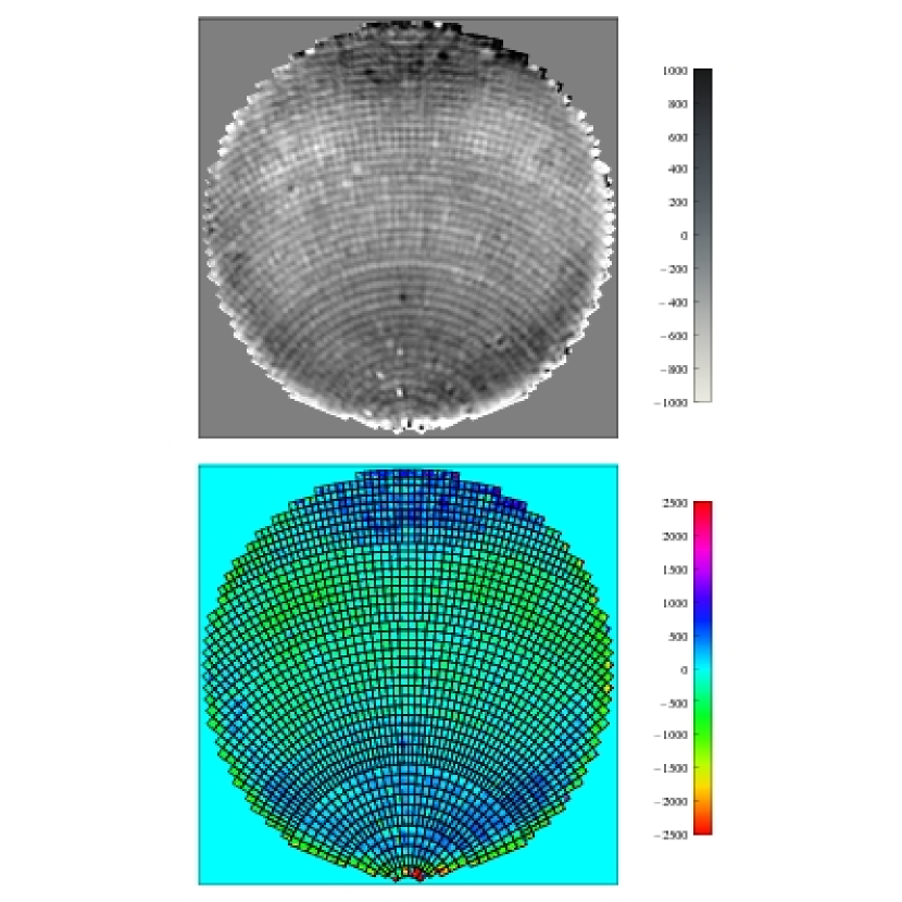
Figure 2: (Top) The Sept. 11, 2009, GBT holography surface error map, ring-filtered and Zernike-restored (i.e., the same as Figure 2b, but with the fifty-five term Zernike polynomial model added back in). (Bottom) Same as above but displayed in color, with the GBT panel layout superimposed. The plot legends are labeled in microns.

Figure 1 shows our Sept. 11, 2009, Zernike-removed surface error map before and after diffraction ring removal. Figure 2 shows that map with the Zernike model restored.

5 Results

5.1 Surface maps and adjustments

In our analysis we have no way of separating subreflector surface errors from main reflector errors. The manufacturing errors of the subreflector panels were held to under $<50\,\mu$m r.m.s., and the achievement of the $100\,\mu$m r.m.s. overall surface accuracy specification for the subreflector—including panel setting—was verified by photogrammetry before telescope commissioning (ca. 2000). The contemporaneous photogrammetric survey measurements of the primary surface actuator control points (in their home positions) had, on the other hand, r.m.s. errors of order twice as large according to estimates provided by the contractor (Geodetic Systems, Inc.,, 2011). Our working assumption is that primary surface errors are dominant. In principle, though, the contribution due to large-scale surface errors on the subreflector can be corrected by adjusting the main reflector.

In the typical holography map, surface features on the primary mirror as small as 0.5 m are visible, compared to the typical panel size of 2 m by 2.5 m. A number of large features coincident with specific actuators were immediately identified, and soon traced to electrical problems either with the actuator motors, their position sensors, or the associated cabling. These problems were repaired during the following months as the campaign continued through several iterations of holography mapping, surface adjustments, and radiometric testing at 90 GHz with the MUSTANG bolometer camera (Dicker et al., 2008).

The surface adjustments take the form of adjustments to the actuator home positions stored in a telescope configuration file. We have also performed manual adjustments of the panel mounting screws at two sets of panel corners which showed particularly noticeable errors not correctable by motion of the associated actuator, each of which are shared by (up to) four panels.

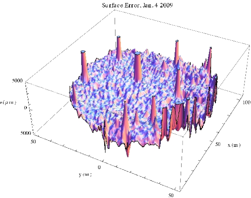
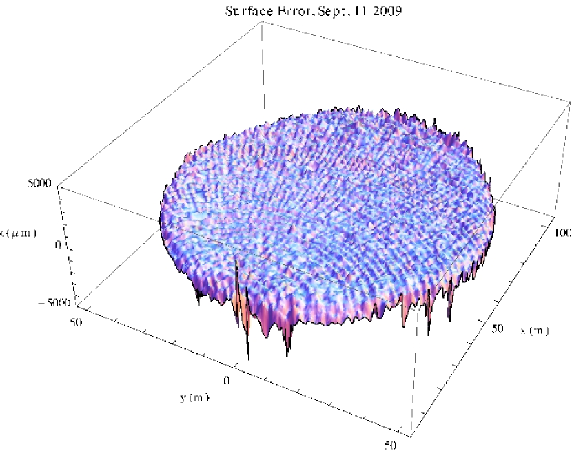
Figure 3: Surface error map derived from the January 4, 2009 holography data (left), compared with the September 11, 2009 map (right), each shown in three-dimensional perspective. Most of the gross outliers which are evident in the January map occur in the regions of influence of malfunctioning actuators. However, a few of the outliers on the outer edge of the dish are due to shimming adjustments made to actuator mounting points following the photogrammetric survey performed in June of 2000. An actuator which is far out of position will result in image artifacts (e.g., ripple effects) that contaminate the derived surface map well beyond the region of mechanical influence of the problem actuator. All 2209 primary surface actuators are believed to have been functioning correctly during the September 11, 2009 observation session.

Our first successful high-resolution GBT holography map was acquired on January 4, 2009. The surface error map derived from this session is shown in the left-hand panel of Figure 3. A large number of outliers are evident in this three-dimensional perspective display. Most of the gross outliers occur in the regions of influence of malfunctioning actuators. A few of the outliers on the right-hand, outer edge of the dish are due to shimming adjustments which were made following the photogrammetric survey performed at the end of the telescope construction period, in June 2000. Grossly malfunctioning actuators can result in image artifacts (e.g., ripple effects) which contaminate the derived surface map well beyond the area of mechanical influence of any particular problem actuator.

Most of the malfunctioning actuators were repaired during the late winter and the spring months of 2009. Some actuator problems were intermittent and took relatively longer to diagnose; however, all were fully functional by the end of summer. Physical access to actuators, which is via cable-supported catwalks, is time-consuming and sometimes logistically difficult. However, the problems due to shimming cleared up immediately, following the application of the first high-resolution holography-based actuator zero-point corrections based on the January 4 holography map, as was verified by the first follow-up holography session on February 9.

5.2 Surface accuracy improvements

Twenty-one successful holography mapping sessions were conducted between February and September, 2009. The first couple of iterations of mapping and surface adjustments produced marked improvements in surface accuracy. Following that, further substantial improvements followed only from holography data acquired under the most favorable meteorological conditions. Each high-resolution map required three to four hours of continuous observation. The most useful maps (for surface setting) were acquired only during the dead of night, during conditions of stable ambient temperature, near thermal equilibrium (i.e., after the daytime thermal effects had damped out; ideally inside a period of a few days prevailing overcast), low winds, and good telescope pointing. Data obtained during sub-optimal conditions (e.g., post-sunrise, as well as clear, cold night) were useful also, particularly in recognizing the repetitive patterns of thermal-gradient induced and gravitationally induced systematic panel distortions (see §5.4).

In the presence of extreme outliers due to malfunctioning actuators, we found the raw r.m.s. statistic not to be generally useful as a summary measure of surface accuracy, because in this case it is not reflective of “typical” surface roughness and is not a reliable predictor of radiometric-equivalent surface accuracy. However, we found the median absolute deviation about the median residual, commonly known as the MAD estimator (Hampel et al., 1986), to be highly useful. For a normal distribution, the MAD is 1.4826 times the standard deviation. In our work, we found found the raw median absolute deviation surface statistic, scaled by 1.4826, to be in relatively close agreement with a “masked” root-mean square statistic, where “masking” implies giving zero weight to all grid points within, say, a 2.5-m radius of any problem actuator.

In order to predict the radiometric efficiency for any standard GBT Gregorian receiver it is also useful to compute weighted r.m.s. statistics, with the weights corresponding to the standard feed illumination taper of $-13$ dB. For comparison with MUSTANG measurements, it is useful to compute an unweighted r.m.s. over the central 90-m diameter of the dish, corresponding to the Lyot stop of the MUSTANG optics. (MUSTANG does not use a tapered illumination pattern.)

Because of the effects of the diffraction rings, which were discussed in §4.5, we made slower progress in improving the outer portion of the surface than the inner portion. As we proceeded we found the combination of an inner MAD (or masked r.m.s.) statistic (computed, say, for radii $r<28$ m) and the corresponding “outer” statistic (for $r>28$ m) to be useful in measuring the relative progress in improving both parts of the dish. (We chose $r=28$ m because that was the smallest radius into which we were generally able to distinguish individual rings for the empirical diffraction ring fitting; we also tabulated the statistics for $r=36.7$ m, because half of the actuators are within that radius and half are outside.)

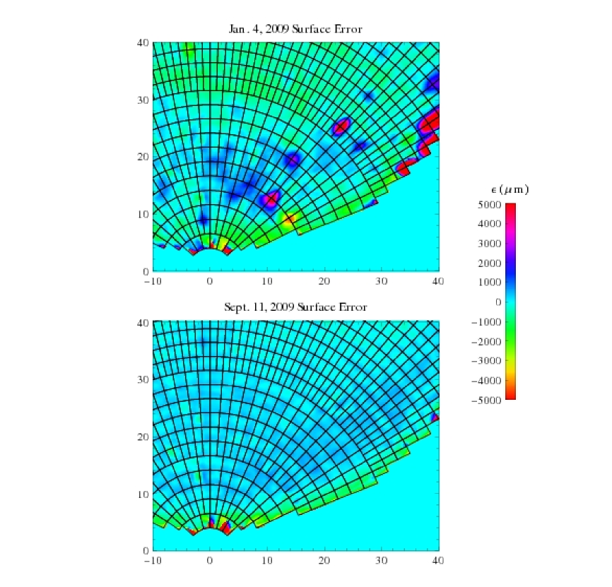
Figure 4: Detailed comparison of the surface error maps derived from January 4 and September 11, 2009 holography data, showing a portion of the surface near the paraboloid vertex. At top, the brightest two red interior globular “blobs” (in Hoops 6 and 13, counting from the vertex) are prototypical examples of the actuator influence functions at transition tiers (Hoop 6, the blob appearing pear-shaped) and at regular panel intersections (Hoop 13, the blob radially elongated). The persistent features in Tier 1 (similar in both maps) are due to permanent damage from ice that has fallen from the feed arm, and to incidents which involved mechanical interference with the access platform. Additional ice damage is present in Tiers 2, 4, and 6 and is evident in the holography maps when a more sensitive transfer function is used for the display.

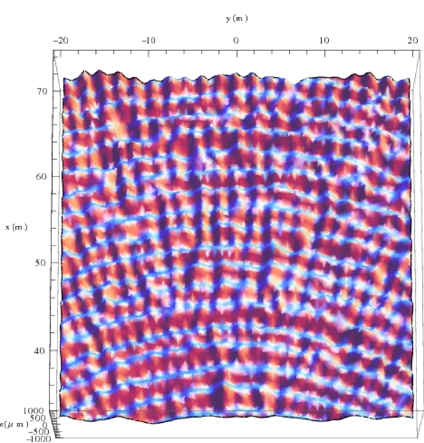
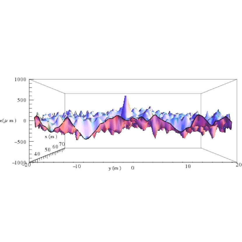
Figure 5: Three-dimensional perspective plots showing—in greater detail than Figures 3 and 4—the central $40{\rm\,m}\times 40{\rm\,m}$ region of the September 11, 2009 surface error map. This area includes the central portions of seventeen consecutive panel tiers (Tiers 13 through 29). These tiers can easily be distinguished via the trough-like patterns of thermal and gravitational sag, which are discussed in §5.4.

The right-hand panel in Figure 3 shows the surface error map from September 11, 2009, near the end of our holography campaign. A more detailed, localized comparison of the beginning and end results is shown in Figure 4, in which an overlay is superimposed to show the panel layout. Figure 5 shows detailed perspective plots of the central portion of the September 11, 2009 map.

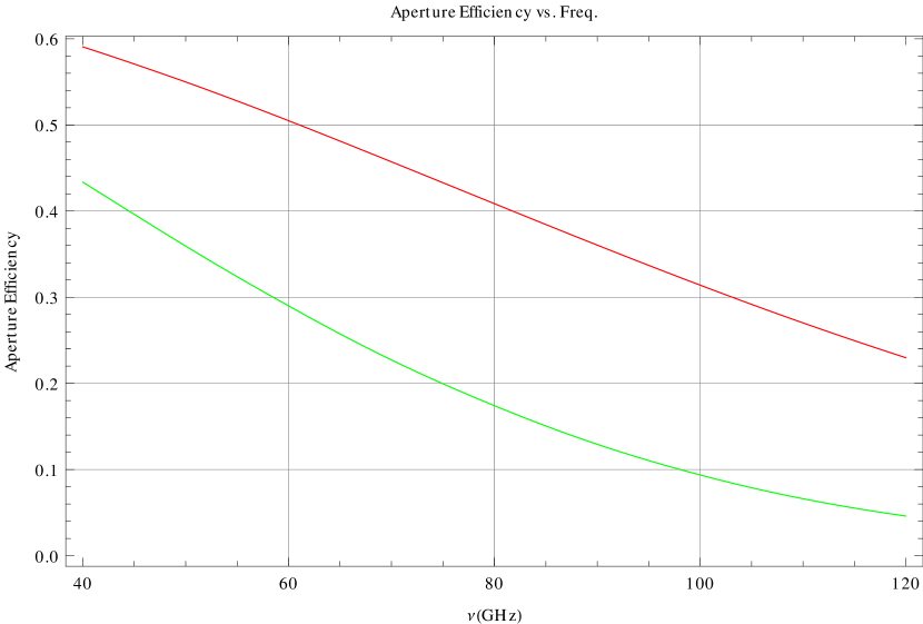
Figure 6: Predicted aperture efficiency vs. frequency curves for the GBT with the surface as measured on January 4, 2009 (lower curve, green), and September 11, 2009 (upper curve, red), assuming illumination of the full 100-m primary aperture by a feed with the standard $-13$ dB edge taper.

Figure 6 shows the aperture efficiency vs. frequency curves that we would predict based on the January 4 and September 11, 2009 GBT holographically measured surfaces, for astronomical observations using a receiver with the standard $-13$ dB edge taper. These predictions are compared with actual radiometric observations in the next section. To calculate the gain, we fit an interpolation function to the measured (phase-unwrapped) holography surface error distribution and performed the aperture-plane integration defined by Equation 1 of Ruze (1966). The peaks in the gain curves occur at 75.2 GHz (91.9 dB) and 119.4 GHz (96.6 dB) for the January 4 and September 11 surfaces, respectively. For the aperture-efficiency calculation we included a diffraction loss based on geometric theory of diffraction (GTD) calculations by Srikanth (1994).

A complete list of successful nighttime holography sessions, representing the data acquired under the best observing conditions, is given in Table 1. The final column in the table shows the r.m.s. surface error (in the normal direction) estimated from the holography map (diffraction ring corrected, and low-order Zernike polynomial terms removed), with the r.m.s. computed over the entire aperture ($r<50$ m), excluding points within a 2.5-m radius of any grossly malfunctioning actuators. The number of such actuators is shown in Column 3. By midsummer 2009, all the grossly malfunctioning actuators had been repaired. Steady progress was made in improving the surface between January and May of 2009. In the January 2010 map, the observed r.m.s. error is in the same range as that of the summer maps. The mean r.m.s. for the last four sessions is 223 $\mu$m. Table 2 shows the results from two daytime holography mapping sessions. For the daytime sessions the mean r.m.s. is 319 $\mu$m, which is 44% greater than that of the final four nighttime sessions.

The nighttime r.m.s. value implies a total surface r.m.s. of ${\sim}240\,\mu$m, assuming that the residual large-scale component of surface error is ${<}100\,\mu$m r.m.s. This assumption should generally be valid during stable thermal conditions but can be more routinely guaranteed by measuring and compensating for large-scale errors by executing the automatic OOF holography procedure (“AutoOOF”) prior to observations (Hunter et al., 2009).

5.3 Efficiency improvements

Following each round of holography measurements, typically within a few days or weeks, we tested the new surface corrections radiometrically using MUSTANG. The active surface software allows one to quickly load a new configuration file containing the complete list of actuator position offsets. Taking full advantage of this capability, we acquired small images of a bright point source quasar using a “daisy petal” scan pattern, which repeatedly passes through the target position with a steadily advancing sequence of angles of attack. We first acquired an image with the old surface, then with the new surface, and repeating the sequence a few times. The purpose of this test was to confirm the expected increase in the response of the detector as the dish was made more accurate. Prior to each test, we performed OOF holography in order to first measure and correct the surface for the current large-scale deviations (mostly thermal in nature). By doing this step, we could ensure that the “old” surface produced its best signal, and thus any improvement subsequently seen with the “new” surface meant that the smaller-scale surface errors had been reduced. As soon as the improved performance of the “new” surface was confirmed, it was installed for general use by astronomers. As such, several astronomy projects have been able to take advantage of some or all of these surface improvements, especially those using MUSTANG. While many more projects in the current (2010–2011) season are underway, data from some MUSTANG projects from the 2009–2010 season have already been published (Mason et al., 2010; Korngut et al., 2010; Shirley et al., 2011).

During these radiometric tests, we often interspersed measurements of the same quasar using the original January 4, 2009 surface in order to assess the total improvement in the surface since the initiation of the holography campaign. However, because there were many failed actuators in the January 4, 2009 surface, the resulting performance ratio increasingly became an underestimate as these actuators were fixed. We thus decided to construct a surface file which mimicked all the measured large errors due to failed actuators. The total improvement ratio measured in this manner on November 23, 2009 was 2.4 with MUSTANG (90 GHz) and 1.4 with the Q-band receiver (43 GHz). Using the best surface, a gain curve was measured from 15° to 85° elevation at 43 GHz on October 4, 2009 using 3C48 and 3C147 (see Figure 7). A second-order polynomial fit to the data showed a nearly flat curve with a maximum aperture efficiency of 63%, as compared with ${\sim}45\%$ measured several years ago, and consistent with the 1.4 improvement factor. Also, these values imply an improvement in the total surface error from $390\,\mu$m (Nikolic et al., 2007b) to ${\sim}240\,\mu$m rms, which is consistent with the improvement in the measured surface errors in the holography maps themselves. Based on this result, we predict the aperture efficiency at 90 GHz is between $30$–35%. Aperture efficiency measurements with MUSTANG are complicated because this term is degenerate with the receiver optical efficiency; however the best estimates are in agreement. We note that MUSTANG illuminates the telescope surface differently from the other GBT receivers because it has a cold Lyot stop corresponding to a diameter of 90 m, rather than the standard $-13$ dB Gaussian taper at a diameter of 100 m. Thus, although the total illumination efficiency is similar between these instruments, the effective aperture efficiency may differ depending on the distribution of surface errors as a function of radius. In any case, the aperture efficiency prediction will be tested soon using the new W-band feedhorn receiver (68–92 GHz) currently under development (Frayer et al., 2010).

5.4 Modeling of panel-scale effects

The improvement in the surface accuracy of the primary mirror has had a correspondingly beneficial effect on the telescope beam pattern. As a by-product of each holography map, we obtain a high-dynamic range image ($>60$ dB) of the amplitude pattern. As the surface was improved, the level of scattered power was reduced and brought into the main beam. A pair of partial arc-like features began to emerge in the pattern, and they are distinctly evident in the September 11, 2009 map shown in the upper left panel of Figure 8. Because the features appear at a radius of about 0.6 degrees, they must be associated with surface structure on the scale of individual panels (cf. Greve & Morris (2005), Greve et al. (2010), Greve & Bremer (2010)). We reviewed the results of a finite-element analysis of the surface panel design, performed by the manufacturer, who modeled the panel response to gravity and to a front-to-back temperature gradient of $2^{\circ}$ C. Each of these effects produces a systematic effect on the shape of the panel. While gravity produces a sag proportional to the projected gravity vector, temperature gradients produce a sag or bulge depending on the sign of the gradient (von Hoerner, 1971).

We were able to scale the models to the geometry of each panel of the dish. Next, we assembled the model panels into a complete model of the aperture, including systematic panel distortions (for full details, see Schwab & Hunter, 2010). Fourier transformation of this model yields the predicted far-field beam pattern, as shown in the upper right panel of Figure 8. Both the upper and lower arcs at 0.6 degrees and the fainter arcs to the left and right at larger radii are qualitatively reproduced by the model. The September 11, 2009 map was obtained under clear nighttime skies, when the measured panel gradient (from surface to rear ribs) was negative ($-2.69^{\circ}$ C) due to preferential radiative cooling toward the sky. The gradient was estimated using two structural thermometers—one attached to a panel skin in Tier 16 and the other on the backup structure adjacent to this panel. The map of November 21, 2009 (lower left panel of Figure 8) was acquired during morning hours from 8:30 AM–12:30 PM, local time, when the measured gradient was positive ($+5.0^{\circ}$ C) because the the majority of panels were being heated by sunlight. The arcs in the pattern are suppressed. We extracted tier-averaged profiles from the holography surface maps which clearly reveal the change from sagging panels to flat or slightly bulging panels (see Figure 9). We conclude that a positive temperature gradient leads to a mechanical deformation in the panels which serves to counteract the sag due to gravity. However, daytime heating effects lead to larger pointing errors and induce large-scale deviations in the dish which must be actively measured and compensated with OOF holography (Hunter et al., 2009). Nevertheless, it is clear that the best nighttime performance of the dish will be obtained when the panel temperature gradient is minimal, which generally occurs during periods of overcast conditions. Unfortunately, these conditions tend not to be the best for millimeter-wavelength transparency.

6 Summary

We have successfully designed and installed a 12-GHz holography system on the GBT. We have performed a campaign of high-resolution holographic imaging of the telescope aperture that has enabled us to achieve a dramatic reduction in the surface error of the primary mirror. The expected improvements in aperture efficiency have been confirmed. The holography images also reveal the magnitude and direction of the response of the panels to different thermal conditions. The holography system is fully integrated into the GBT control system and continues to be in regular use to monitor the health of the individual actuators, which is essential to support high-frequency observations.

Figure 1: The Sept. 11, 2009, GBT holography surface error map, before (top) and after application (bottom) of our diffraction ring filtering algorithm. Large-scale structure—as represented by a fifty-five term Zernike polynomial fit—was removed from the surface error map prior to diffraction ring removal. The plot legend is labeled in microns.

Figure 7: Plot of GBT aperture efficiency vs. elevation measurements taken at 43.1 GHz on October 4, 2009. Left-circular polarization data are represented by the filled circles (shown in blue); right-circular polarization data by the filled squares (red). Quadratic fits to the data are shown by the solid (blue) and dashed (red) curves, for left- and right-circular polarizations, respectively.

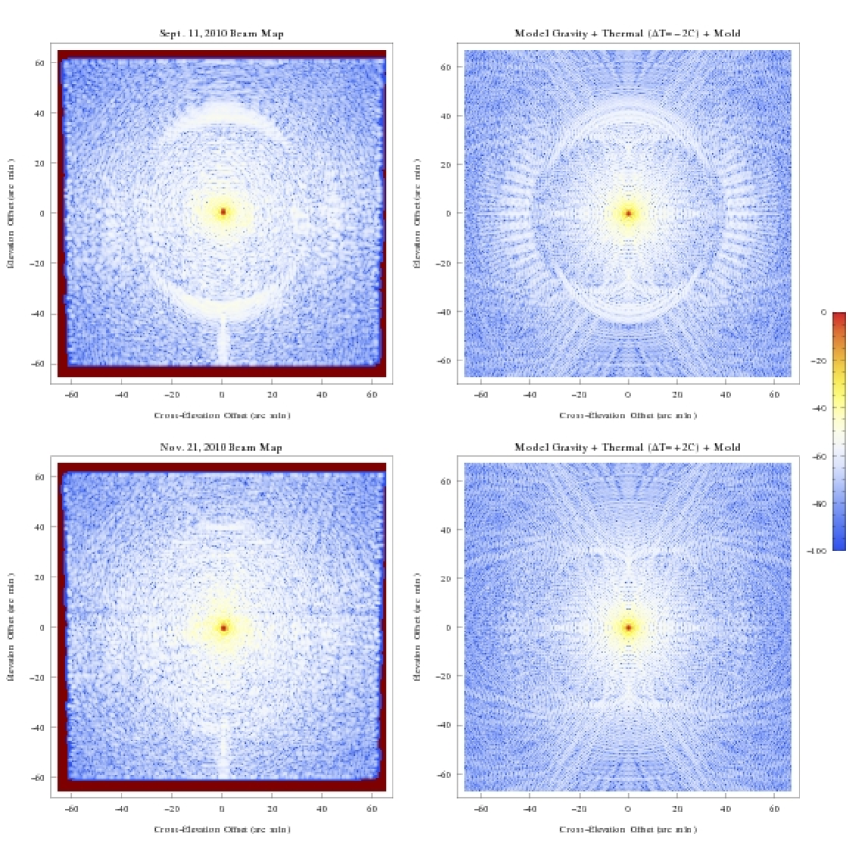
Figure 8: A comparison of observed and model beam patterns: (Upper row) The September 11, 2009 map, on the left, is compared with a model which includes gravitational (elev. $44^{\circ}$), thermal gradient ($\Delta T=-2$ C), and manufacturing mold errors. (Bottom row) The November 21, 2009 daytime map is compared with the model for thermal gradient, $\Delta T=+2$ C. Power in dB (relative to the peak) is represented by the plot legend on the right.

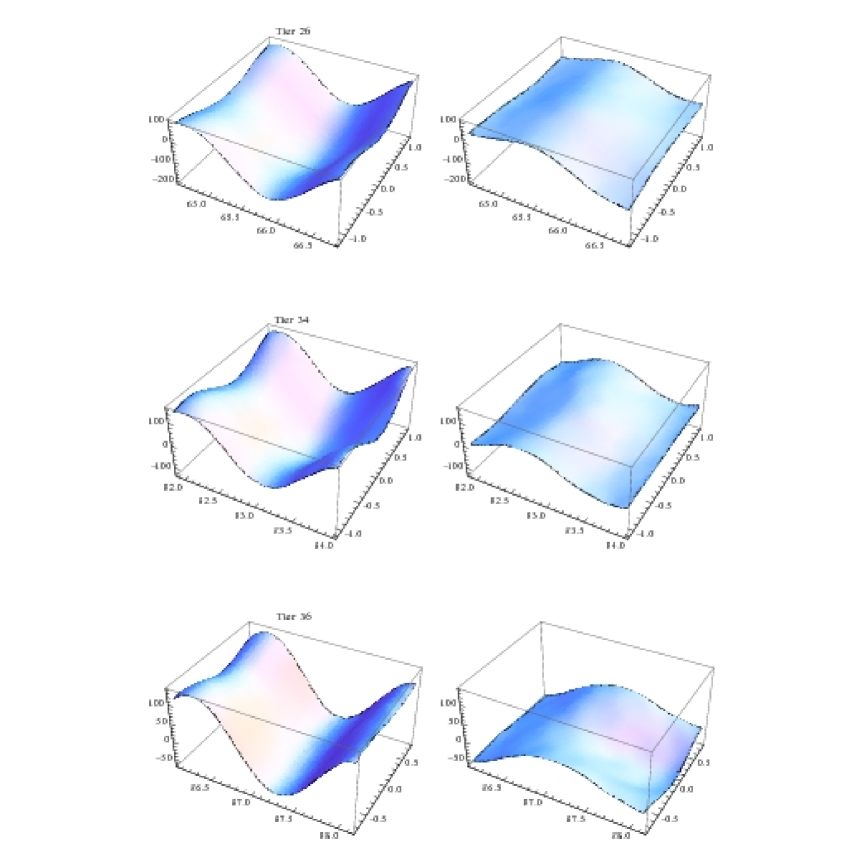
Figure 9: Comparison of tier-average surface error profiles from the September 11, 2009 map, shown at left, and the November 21, 2009 map, at right. The mean gradient $\overline{\Delta T}$ (measured at Tier 16 panel node 16+000) was $-2.69\,{}^{\circ}$C for the September 11 observations and $+5.00\,{}^{\circ}$C on November 21. The vertical axis is labeled in microns; units along the $x$- and $y$-axes are in meters. The selected tiers show the general behavior: negative $\Delta T$ producing a panel sag; and positive, a flattening or a bulge. Results for all tiers are given by Schwab & Hunter (2010), together with results from two other holography sessions.

Table 1: Successful nighttime holography mapping observations

UT Date	UT Start Time	No. Bad Act.	Trimmed r.m.s. ($\mu$m)
2009 Jan 04	05:57	21	423
2009 Feb 06	05:24	6	424
2009 Mar 15	08:46	4	321
2009 May 27	00:13	12	214
2009 Aug 16	05:18	0	210
2009 Sep 11	03:42	0	226
2010 Jan 21	08:33	3	239

Table 2: Daytime holography mapping observations

UT Date	UT Start Time	No. Bad Act.	Trimmed r.m.s. ($\mu$m)
2009 Nov 21	13:24	2	309
2010 May 27	11:22	4	329

References

- Baars et al. (2007) Baars, J. W. M., Lucas, R., Mangum, J. G., & Lopez-Perez, J. A. 2007, IEEE Antennas & Propagation Mag., 47(5), 24; also arXiv:0710.4244
- Balasubramanyam et al. (2009) Balasubramanyam, R., Venkatesh, S., & Raju, S. B. 2009, in ASP Conf. Ser. 407, The Low-Frequency Radio Universe, ed. D. J. Saikia, D. A. Green, Y. Gupta, & T. Venturi, (San Francisco: ASP), 434
- Bennett et al. (1976) Bennett, J. C., Anderson, A. P., McInnes, P. A., & Whitaker, A. J. T. 1976, IEEE Trans. Antennas & Propagation, AP-24, 295
- Constantikes (2004) Constantikes, K. 2004, in ASP Conf. Ser. 314, Astronomical Data Analysis Software and Systems XIII, ed. F. Ochsenbein, M. G. Allen, & D. Egret, (San Francisco: ASP), 689
- Constantikes (2007) Constantikes, K. 2007, USNC/CNC/URSI North American Radio Science Meeting in Ottawa, Canada, July 2007
- Dicker et al. (2008) Dicker, S. R., Korngut, P. M., Mason, B. S, Ade, P. A. R., Aguirre, J., Ames, T. J., Benford, D. J., Chen, T. C., Chervenak, J. A., Cotton, W. D., Devlin, M. J., Figueroa-Feliciano, E., Irwin, K. D., Maher, S., Mello, M., Moseley, S. H., Tally, D. J., Tucker, C., & White, S. D. 2008, Proc. SPIE, 7020:702005
- Frayer et al. (2010) Frayer, D. T., O’Neil, K., Lockman, J., Hunter, T., Wootten, A., Maddalena, R., Ghigo, F., & Langston, G., American Astronomical Society Meeting Abstracts, 216, #414.01
- Geodetic Systems, Inc., (2011) Geodetic Systems, Inc., 2011, Melbourne, FL; http://www.geodetic.com/about/
- Ghiglia & Pritt (1998) Ghiglia, D. C. and Pritt, M. D. 1998, Two-Dimensional Phase Unwrapping: Theory, Algorithms, and Software, (New York: Wiley)
- Grahl et al. (1986) Grahl, B. H., Godwin, M. P., & Schoessow, E. P. 1986, A&A, 167, 390
- Greve & Morris (2005) Greve, A. & Morris, D. 2005, IEEE Trans. Antennas & Propagation, AP-53(6), 2123
- Greve et al. (2010) Greve, A., Morris, D., Peñalver, J., Thum, C., & Bremer, M. 2010, IEEE Trans. Antennas & Propagation, AP-58(3), 959
- Greve & Bremer (2010) Greve, A. & Bremer, M. 2010, Thermal Design and Thermal Behaviour of Radio Telescopes and their Enclosures, (Heidelberg: Springer)
- Hampel et al. (1986) Hampel, F. R., Ronchetti, E. M, Rousseeuw, P. J., & Stahel, W. A. 1986, Robust Statistics: The Approach Based on Influence Functions, (New York: Wiley)
- Hunter et al. (2009) Hunter, T. R., Mello, M., Nikolic, B., Mason, B., Schwab, F., Ghigo, F., & Dicker, S. 2009, 2009 USNC/URSI Annual Meeting, 45
- Korngut et al. (2010) Korngut, P. M., Dicker, S. R., Reese, E. D., Mason, B. S., Devlin, M. J., Mroczkowski, T., Sarazin, C. L., Sun, M., & Sievers, J. 2010, arXiv:1010.5494
- Lacasse (1998) Lacasse, R. J. 1998, Proc. SPIE, 3351, 310
- Maciolek & Maddalena (2000) Maciolek, A. A., & Maddalena, R. J. 2000, BAAS, 32, 1555
- Mangum et al. (2007) Mangum, J. G., Emerson, D. T., & Greisen, E. W. 2007, A&A, 474, 679
- Mason et al. (2010) Mason, B. S., Dicker, S.R., Korngut, P. M., Devlin, M. J., Cotton, W. D., Koch, P. M., Molnar, S. M., Sievers, J., Aguirre, J. E., Benford, D., Staguhn, J. G., Moseley, H., Irwin, K. D., & Ade, P. 2010, ApJ, 716, 739
- Nikolic et al. (2007a) Nikolic, B., Hills, R. E., & Richer, J. S. 2007a, A&A, 465, 679
- Nikolic et al. (2007b) Nikolic, B., Prestage, R. M., Balser, D. S., Chandler, C. J., & Hills, R. E. 2007b, A&A, 465, 685
- O’Neil et al. (2006) O’Neil, K., Shelton, A. L., Radziwill, N. M., & Prestage, R. M. 2006, in ASP Conf. Ser. 351, Astronomical Data Analysis Software and Systems XV, ed. C. Gabriel, C. Arviset, D. Ponz, & E. Solano, (San Francisco: ASP), 719
- Parker et al. (2005) Parker, D. H., Anderson, R., Egan, D., Fakes, T., Radcliff, B., & Shelton, J. W. 2005, Precision Engineering, 29, 354
- Percival & Walden (1993) Percival, D. B. and Walden, A. T. 1993, Spectral Analysis for Physical Applications: Multitaper and Conventional Univariate Techniques, (Cambridge: Cambridge Univ. Press)
- Prestage et al. (2009) Prestage, R. M., Constantikes, K. T., Hunter, T. R., King, L. J., Lacasse, R. J., Lockman, F. J., & Norrod, R. D. 2009, Proc. IEEE, 97, 1382
- Radford et al. (1996) Radford, S. J. E., Reiland, G., & Shillue, B. 1996, PASP, 108, 441
-
RSI (1992)
Radiation Systems Inc., 1992, Technical
Memo 101,
https://safe.nrao.edu/wiki/pub/GB/PTCS/LoralTechnicalMemos/TM101.pdf - Rahmat-Samii (1985) Rahmit-Samii, Y. 1985, IEEE Trans. Antennas & Propagation, AP-33, 1194
- Ries et al. (2011) Ries, P., Hunter, T. R., Constantikes, K. T., Brandt, J. J., Ghigo, F. D., Prestage, R. M., Ray, J., & Schwab, F. R., 2011, PASP, to appear; arXiv:0710.4244v1
- Rochblatt & Rahmat-Samii (1991) Rochblatt, D. J., & Rahmat-Samii, Y. 1991, IEEE Trans. Antennas & Propagation, AP-39, 933
- Ruze (1966) Ruze, J. 1966, Proc. IEEE, 54, 633
- Schwab (1984) Schwab, F. R. 1984, in Indirect Imaging, ed. J. A. Roberts, (Cambridge: Cambridge Univ. Press), 333
-
Schwab (1990)
Schwab, F. R. 1990, GBT Memo 28,
NRAO, Green Bank, WV;
https://safe.nrao.edu/wiki/pub/GB/Knowledge/GBTMemos/GBT_Memo_28.pdf - Schwab (2008) Schwab, F. R. 2008, PTCS Project Note 62, NRAO, Green Bank, WV
- Schwab & Hunter (2010) Schwab, F. R. & Hunter, T. 2010, GBT Memo. 271, NRAO, Green Bank, WV
- Scott & Ryle (1977) Scott, P. F., & Ryle, M. 1977, MNRAS, 178, 539
- Shirley et al. (2011) Shirley, Y. L., Mason, B. S., Mangum, J. G., Bolin, D. E., Devlin, M. J., Dicker, S. R., & Korngut, P. M. 2011, AJ, 141, 39
- Srikanth (1994) Srikanth, S. 1994, GBT Memo. 215, NRAO, Green Bank, WV
- von Hoerner (1971) von Hoerner, S. 1971, Largest Feasible Steerable Telescope Report No. 36, NRAO, Green Bank, WV; https://safe.nrao.edu/wiki/pub/GB/PTCS/NLSRTMemos/65M_36.pdf
- Wolfram Research (2010) Wolfram Research, Inc., 2010, Mathematica, Version 8.0, Champaign, IL
- Zemax Development Corp. (2010) Zemax Development Corp., 2010, Zemax: Software for Optical System Design, Bellevue, WA; http://www.zemax.com