Influence of polydispersity on micromechanics of granular materials

Abstract

We study the effect of polydispersity on the macroscopic physical properties of granular packings in two and three dimensions. A mean-field approach is developed to approximate the macroscale quantities as functions of the microscopic ones. We show that the trace of the fabric and stress tensors are proportional to the mean packing properties (e.g. packing fraction, average coordination number, and average normal force) and dimensionless correction factors, which depend only on the moments of the particle-size distribution. Similar results are obtained for the elements of the stiffness tensor of isotropic packings in the linear affine response regime. Our theoretical predictions are in good agreement with the simulation results.

I Introduction

The physics of granular media has received a lot of attention because of its scientific challenges and industrial relevance. The structural and dynamical properties of granular materials differ from those of ordinary solids, liquids, or gases due to nonlinearity and disorder deGennes99 ; Jaeger96 ; Hinrichsen04 . On the microscopic level, a static assembly of grains consists of particles which interact with their neighbors in order to prevent interpenetration. In spite of the uniform density of granular packings, the resulting contact and force networks between particles are highly inhomogeneous Radjai96 ; Makse00 ; Ostojic06 , leading to many intriguing phenomena in these systems. Describing the behavior via micromechanical approaches, in which the discrete nature of the system is taken into account, is thus commonly preferred to continuum-mechanical approaches where some heuristic assumptions have to be made in order to construct the constitutive equations for macroscopic fields. One can then express the macroscopic physical quantities in terms of the microscale ones. For example, thermal and electrical conductivities are related to the trace of the fabric tensor, a micro-geometrical probability of the orientations of contacts. While the relationship between macroscopic and microscopic properties of granular media has been studied widely deGennes99 ; Hinrichsen04 ; Luding04 , the question remains as to what extent the macroscale quantities are sensitive to the micro-scale details, and how large is the error introduced in the calculation of the “observable quantities” by taking into account only the average packing properties.

Granular materials in nature and industry consist of particles with the common property of polydispersity. It is known that size polydispersity affects the mechanical behavior of granular systems (e.g. shear strength) Wackenhut05 ; Voivret09 as well as their space-filling properties (e.g. packing fraction) Herrmann03 ; Voivret07 , which are crucial in many chemical processes like absorption, filtering, etc. Polydispersity in most studies, so far, has been restricted to narrow size distributions mainly to prevent long-range structural order; however, there are a few studies where broader ranges of particle-size distribution are investigated Voivret09 ; Voivret07 ; Dodds02 ; Ogarko12 . In this paper, we address the question of how deviation from the monodisperse case influences the macroscopic properties of granular assemblies.

We consider a special case of spherical particles [or disks in two dimensions (2D)] allowing for analytical calculations. The main goal is to develop a mean-field approach to calculate the desired microscopic quantities, such as the trace of the fabric and stress tensors, and the elements of the stiffness tensor in two- and three-dimensional polydisperse granular systems. These quantities are directly connected to macroscopic quantities such as thermal and electrical conductivities, isotropic pressure, and bulk and shear moduli. A similar analytical approach has been already used in Ref. Madadi04 to calculate the trace of the fabric tensor in 2D packings, where it turned out that the trace of fabric is factorized into three contributions: (i) the volume fraction, (ii) the mean coordination number, and (iii) a dimensionless correction factor which only depends on the particle-size distribution. Using a similar approach, here we investigate also the stress and stiffness tensors and extend the method to 3D cases. In order to compare the analytical results with numerical simulations, we first construct static packings of grains using contact dynamics simulations Moreau94 ; Jean99 ; Brendel04 . The initial dilute systems of rigid particles are compressed by imposing a confining pressure to get the final static homogeneous packings Shaebani09 . Comparisons are then made between the results of our mean-field model and the exact values obtained from the numerical simulations.

This work is organized in the following manner: The fabric tensor of a polydisperse assembly of spherical particles is investigated in Sec. II, and a mean-field approach is introduced to calculate the trace of fabric. We present the analytical results for the calculation of the stress tensor in Sec. III, and the same approach is used in Sec. IV to investigate the stiffness tensor elements in frictionless isotropic packings. In Sec. V, the analytical calculations are compared to numerical simulations of corresponding packings of polydisperse particles. Finally, we discuss and conclude the results in Sec. VI. Detailed calculations for two-dimensional packings of disks are presented in the Appendix.

II Fabric tensor

II.1 Single-particle case

Various definitions of the fabric tensor have been used in the literature to describe the spatial arrangement of the particles in a granular assembly Goddard86 ; Chang88 ; Rothenburg81 . The fabric tensor of the second order for one particle is defined as Mehrabadi82 ; Latzel00 ; Madadi04

$${\mathit{h}}^{{}^{p}}_{{}_{\alpha\beta}}=\sum_{c=1}^{C_{p}}\frac{l^{{}^{pc}}_{\alpha}}{|\vec{l}^{{}^{pc}}|}\frac{l^{{}^{pc}}_{\beta}}{|\vec{l}^{{}^{pc}}|},$$ (1)

where $C_{p}$ is the number of contacts of particle $p$, and $l^{{}^{pc}}_{\alpha}$ is the $\alpha$ component of the branch vector $\vec{l}^{{}^{\;pc}}$, connecting the center of particle $p$ to its contact $c$. In the case of spherical particles, the unit branch vector $\vec{l}^{{}^{\;pc}}/|\vec{l}^{{}^{\;pc}}|$ and the unit normal vector $\hat{n}^{{}^{pc}}$ at contact $c$ are identical. The trace of the single-particle fabric tensor in a $D$-dimensional system is

$${\mathit{h}}^{{}^{p}}_{{}_{\alpha\alpha}}=\sum_{c=1}^{C_{p}}\sum_{\alpha=1}^{D}\frac{l^{{}^{pc}}_{\alpha}}{|\vec{l}^{{}^{pc}}|}\frac{l^{{}^{pc}}_{\alpha}}{|\vec{l}^{{}^{pc}}|}=C_{p},$$ (2)

i.e. the number of contacts of particle $p$.

II.2 Many-particle case

The average fabric tensor $\langle{\mathit{h}}_{{}_{\alpha\beta}}\rangle_{{}_{V}}$ enables us to describe the global contact network in a given volume $V$. Assuming that the contribution of particle $p$ (lying inside $V$) to the average fabric tensor is proportional to its volume $V_{p}$, we obtain

$$\langle{\mathit{h}}_{{}_{\alpha\beta}}\rangle_{{}_{V}}=\frac{1}{V}\sum^{N}_{p=1}V_{p}{\mathit{h}}^{{}^{p}}_{{}_{\alpha\beta}},$$ (3)

where the sum runs over all particles lying inside $V$, and $\langle\cdot\cdot\cdot\rangle_{{}_{V}}$ denotes the volume weighted average. Using Eq. (2) to calculate the trace of the average fabric tensor, we get

$$\langle{\mathit{h}}_{{}_{\alpha\alpha}}\rangle_{{}_{V}}=\frac{1}{V}\sum^{N}_{p=1}V_{p}C_{p},$$ (4)

which can be interpreted as the contact number density. Alternative possibilities, e.g. using the volume of the polygon that contains the particle (obtained e.g. via Voronoi tessellation), or introducing constant prefactors or slightly different volume contributions are not discussed here (see Refs. Goddard86 ; Chang88 ; Cowin85 ; Duran10 for more details). In a monodisperse packing, Eq. (4) for identical particles is reduced to $\langle{\mathit{h}}_{{}_{\alpha\alpha}}\rangle_{{}_{V}}\!=\!\phi z$, where $\phi$ is the packing fraction ($\phi=\sum_{p}V_{p}/V$), and $z$ is the average coordination number ($z=\sum_{p}C_{p}/N$). We note that only “real” contacts contribute to the calculation of $z$, and geometrical neighbors without a permanent physical contact, which do not contribute in the fabric and force carrying structures, are not considered here.

II.3 Polydispersity

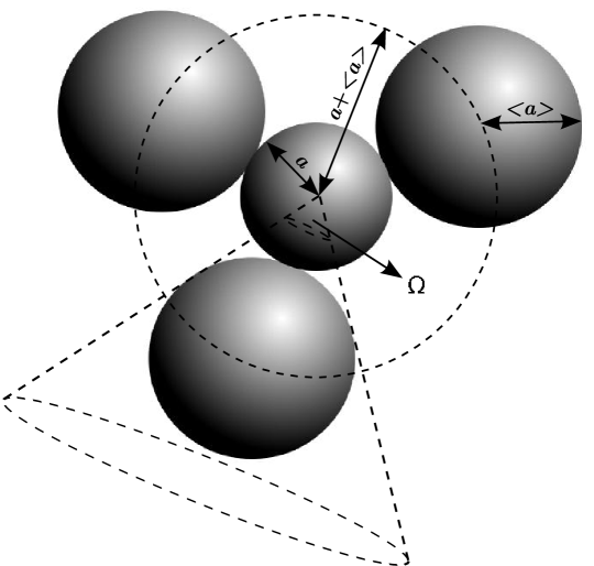
Figure 1: Schematic picture showing a typical particle with radius $a$ surrounded by identical particles of average radius $\langle a\rangle$ in a 3D packing of spheres.

For an accurate evaluation of the trace of the average fabric tensor in a polydisperse granular packing, one should take into account the contributions from all particles. However, if the distribution function of particle radii is known, $\langle{\mathit{h}}_{{}_{\alpha\alpha}}\rangle_{{}_{V}}$ can be approximated as a function of the moments of the size distribution. We assume a polydisperse distribution of particle radii with probability $f(a)da$ to find the radius between $a$ and $a+da$, and with $\int_{0}^{\infty}f(a)da=1$. The continuum limit of Eq. (4) is then given by

$$\langle{\mathit{h}}_{{}_{\alpha\alpha}}\rangle_{{}_{V}}=\frac{N}{V}\int_{0}^{\infty}V(a)C(a)f(a)da.$$ (5)

Here, $C(a)$ is the average coordination number of particles with radius $a$. We evaluate $C(a)$ using a mean-field approach similar to the one proposed in Ouchiyama81 and used already in Madadi04 to study the trace of the fabric tensor. In the following, we concentrate on the case of spherical particles in three-dimensional systems (see the detailed calculations for two-dimensional packings of disks in the Appendix). Let us suppose that each particle in the polydisperse granular medium is surrounded by identical particles of average radius $\langle a\rangle$ (see Fig. 1), where $\langle a\rangle\!=\!\int_{{}_{0}}^{{}^{\infty}}\!\!\!af(a)da$. The surface of a reference particle of radius $a$ is then shielded by its $C(a)$ neighboring particles of radius $\langle a\rangle$. The space angle covered by a neighboring particle on the reference particle in a three-dimensional packing of spheres is

$$\Omega(a)=2\pi\Bigg{(}1-\frac{\sqrt{(a+\langle a\rangle)^{2}-\langle a\rangle^{2}}}{a+\langle a\rangle}\Bigg{)}.$$ (6)

The total fraction of shielded surface, also called linear compacity, is obtained as

$$c_{s}(a)=\frac{1}{4\pi a^{2}}\sum_{i=1}^{C(a)}\Omega(a)a^{2}=\Omega(a)C(a)/4\pi.$$ (7)

Now, another basic assumption is that the total fraction of shielded surface $c_{s}$ is independent of the particle radius $a$. As a result, the expected mean coordination number becomes

$$z=\int_{0}^{\infty}\!\!\!C(a)f(a)da=4\pi c_{s}q_{{}_{0}},$$ (8)

with $q_{{}_{0}}{=}\int_{{}_{0}}^{{}^{\infty}}\!\!f(a)/\Omega(a)da$. Using Eqs. (7) and (8) one finds

$$C(a)=\frac{z}{q_{{}_{0}}\Omega(a)}.$$ (9)

The trace of the fabric tensor for a polydisperse packing is then obtained by substitution of Eq. (9) in Eq. (5),

$$\langle{\mathit{h}}_{{}_{\alpha\alpha}}\rangle_{{}_{V}}=\phi zg_{{}_{1}},$$ (10)

where the correction factor $g_{{}_{1}}$ is defined as

$$g_{{}_{1}}=\frac{\displaystyle\int_{0}^{\infty}V(a)\frac{f(a)}{\Omega(a)}da}{q_{{}_{0}}\displaystyle\int_{0}^{\infty}V(a)f(a)da}=\frac{\langle a^{3}\rangle_{{}_{g}}}{\langle a^{3}\rangle}$$ (11)

Here, $\langle a^{k}\rangle\!$ and $\langle a^{k}\rangle_{{}_{g}}$ denote the $k$th moments of the size distribution $f(a)$ and the modified distribution $f(a)/\Omega(a)$ normalized by $q_{{}_{0}}$, respectively. We note that $g_{{}_{1}}$ depends only on the size distribution function $f(a)$.

II.4 Narrow size distributions

By introducing $\epsilon(a){=}a/\langle a\rangle{-}1$, which ranges between $-1$ and $\infty$ depending on the choice of $a$, Eq. (6) can be written as

$$\Omega(a)=2\pi\Bigg{(}1-\frac{\sqrt{\epsilon^{2}+4\epsilon+3}}{2+\epsilon}\Bigg{)}.$$ (12)

Indeed, $\epsilon(a)$ quantifies the deviation from the mean particle size $\langle a\rangle$ [e.g. $\epsilon(a)$ equals zero in the monodisperse case]. Hence, for narrow size distributions, we approximate $1/\Omega(a)$ by Taylor expansion around $\epsilon{=}0$ (corresponding to Taylor expansion around $a{=}\langle a\rangle$). By Taylor expansion to the second order in $\epsilon$, one obtains

$$\frac{1}{\Omega(a)}\simeq A_{{}_{1}}+B_{{}_{1}}\epsilon+C_{{}_{1}}\epsilon^{2},$$ (13)

with $A_{{}_{1}}\!\!=\!\frac{1}{(2-\sqrt{3})\pi}$, $B_{{}_{1}}\!\!=\!\frac{1}{2\sqrt{3}(2-\sqrt{3})^{2}\pi}$, and $C_{{}_{1}}\!\!=\!\frac{1}{3(3+\sqrt{3})(2-\sqrt{3})^{2}\pi}$. The first-order approximation deviates significantly from the exact value (see Fig. 2). However, the second-order expansion provides a good approximation with less than $1\%$ error in the range $-0.5\!<\!\epsilon\!<\!7.5$ (or $0.5\langle a\rangle\!<\!a\!<\!8.5\langle a\rangle$).

Figure 2: $1/\Omega(a)$ as a function of $\epsilon$. The exact value (solid line) is compared with the first-order (dashed line) and second-order (dash-dotted line) approximations. The inset shows more clearly the deviation of the approximations from the exact value.

Therefore, the correction factor [Eq. (11)] for narrow size distributions becomes

$$g_{{}_{1}}\!\simeq\!\frac{(A_{{}_{1}}{-}B_{{}_{1}}{+}C_{{}_{1}}){+}(B_{{}_{1}}{-}2C_{{}_{1}})\frac{\big{\langle}\displaystyle{a}^{4}\big{\rangle}}{\big{\langle}\displaystyle{a}\big{\rangle}\big{\langle}\displaystyle{a}^{3}\big{\rangle}}{+}C_{{}_{1}}\frac{\big{\langle}\displaystyle{a}^{5}\big{\rangle}}{\big{\langle}\displaystyle{a}\big{\rangle}^{2}\big{\langle}\displaystyle{a}^{3}\big{\rangle}}}{(A_{{}_{1}}{-}C_{{}_{1}}){+}C_{{}_{1}}\frac{\big{\langle}\displaystyle{a}^{2}\big{\rangle}}{\big{\langle}\displaystyle{a}\big{\rangle}^{2}}}.$$ (14)

Equation (14) should account for arbitrarily shaped size distributions $f(a)$ as long as they are not too wide. Note the different nomenclature in Ref. Goncu10 , where the above equation is introduced with different abbreviations and coefficients.

III Stress tensor

III.1 Single-particle case

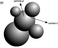
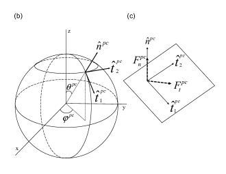
Figure 3: (a) A typical contact $c$ between the reference particle $p$ and its neighboring particle. (b) The contact unit vectors $\hat{n}^{pc}$, $\hat{t}_{1}^{pc}$, and $\hat{t}_{2}^{pc}$. (c) The normal ($F^{pc}_{n}$) and tangential ($F^{pc}_{t}$) components of the contact force $\vec{F}^{{}^{pc}}\!\!\!$.

The micromechanical expressions for the components of the stress tensor $\sigma^{p}_{\alpha\beta}$ of a single particle in a static granular assembly are Christoffersen81 ; Latzel00

$$\sigma^{{}^{p}}_{{}_{\alpha\beta}}=\frac{1}{V_{p}}\sum_{c=1}^{C_{p}}l^{{}^{pc}}_{\alpha}F^{{}^{pc}}_{\beta},$$ (15)

where $\vec{F}^{{}^{pc}}$ is the force exerted on particle $p$ by its neighboring particle at contact $c$.

One could assume in a crude approximation that the force at contact $c$ is equal to $\bar{F}_{n}^{p}\hat{n}^{pc}+\bar{F}_{t_{1}}^{p}{\hat{t}}_{{}_{1}}^{pc}+\bar{F}_{t_{2}}^{p}{\hat{t}}_{{}_{2}}^{pc}$ in a three-dimensional system, where $\bar{F}_{n}^{p}$, $\bar{F}_{t_{1}}^{p}$, and $\bar{F}_{t_{2}}^{p}$ are the average normal and tangential contact forces around the particle $p$, and $\hat{n}^{pc}$, ${\hat{t}}_{{}_{1}}^{pc}$, and ${\hat{t}}_{{}_{2}}^{pc}$ are the normal and tangential unit vectors at contact $c$, respectively. Then the force-averaged stress tensor becomes

$$\widetilde{\sigma}^{{}^{p}}_{{}_{\alpha\beta}}{=}\frac{a_{p}}{V_{p}}\biggl{(}\bar{F}_{n}^{p}\sum_{c=1}^{C_{p}}n^{{}^{pc}}_{\alpha}n^{{}^{pc}}_{\beta}+\bar{F}_{t_{1}}^{p}\sum_{c=1}^{C_{p}}n^{{}^{pc}}_{\alpha}t_{1\beta}^{{}^{pc}}+\bar{F}_{t_{2}}^{p}\sum_{c=1}^{C_{p}}n^{{}^{pc}}_{\alpha}t_{2\beta}^{{}^{pc}}\biggr{)}.$$ (16)

For a spherical grain, we project the contact unit vectors ($\hat{n}^{{}^{pc}}$, $\hat{t}_{{}_{1}}^{{}^{pc}}$, $\hat{t}_{{}_{2}}^{{}^{pc}}$) onto an arbitrary Cartesian coordinate system [Figs. 3(a) and 3(b)], and write the force-averaged stress tensor of a single particle as

$$\widetilde{\sigma}^{{}^{p}}=\frac{a_{p}}{V_{p}}\sum_{c=1}^{C_{p}}\Biggl{[}\bar{F}_{n}^{p}\left(\begin{array}[]{ccc}\;W_{2002}&\;W_{2011}&\;W_{1101}\\ \;W_{2011}&\;W_{2020}&\;W_{1110}\\ \;W_{1101}&\;W_{1110}&\;W_{0200}\end{array}\right)$$ (20)

$$\hskip 12.80365pt+\bar{F}_{t_{1}}^{p}\left(\begin{array}[]{ccc}\;W_{1102}&W_{1111}&\!\!-W_{2001}\\ \;W_{1111}&W_{1120}&\!\!-W_{2010}\\ \;W_{0201}&W_{0210}&\!\!-W_{1100}\end{array}\right)$$ (24)

$$\hskip 12.80365pt+\bar{F}_{t_{2}}^{p}\left(\begin{array}[]{ccc}\!\!\!-W_{1011}&W_{1002}&\;\;\;\;0\\ \!\!\!-W_{1020}&W_{1011}&\;\;\;\;0\\ \!\!\!-W_{0110}&W_{0101}&\;\;\;\;0\end{array}\;\right)\Biggr{]},$$ (28)

where the $W_{mnkl}$ function is defined as

$$W_{mnkl}=\sin^{m}(\theta_{c})\cos^{n}(\theta_{c})\sin^{k}(\varphi_{c})\cos^{l}(\varphi_{c}),$$ (29)

with $0{\leqslant}\theta_{c}{<}\pi$ and $0{\leqslant}\varphi_{c}{<}2\pi$. Using Eq. (16), the trace of the stress tensor becomes

$$\widetilde{\sigma}^{{}^{p}}_{{}_{\alpha\alpha}}{=}\frac{a_{p}}{V_{p}}\sum_{c=1}^{C_{p}}\sum_{\alpha=1}^{3}\biggl{(}\!\!\bar{F}_{n}^{p}n^{{}^{pc}}_{\alpha}n^{{}^{pc}}_{\alpha}{+}\bar{F}_{t_{1}}^{p}n^{{}^{pc}}_{\alpha}t_{1\alpha}^{{}^{pc}}{+}\bar{F}_{t_{2}}^{p}n^{{}^{pc}}_{\alpha}t_{2\alpha}^{{}^{pc}}\!\!\biggr{)}$$

$${=}\displaystyle\frac{a_{p}}{V_{p}}\!\!\displaystyle\sum_{c=1}^{C_{p}}\biggl{(}\!\!\bar{F}_{n}^{p}|\hat{n}^{{}^{pc}}\!|^{{}^{2}}{+}\bar{F}_{t_{1}}^{p}\hat{n}^{{}^{pc}}\!\!\!\!\cdot\hat{t}_{1}^{{}^{pc}}{+}\bar{F}_{t_{2}}^{p}\hat{n}^{{}^{pc}}\!\!\!\!\cdot\hat{t}_{2}^{{}^{pc}}\!\!\biggr{)}{=}\frac{a_{p}}{V_{p}}\bar{F}_{n}^{p}C_{p}.$$

Equation (LABEL:stress-single-trace) remains valid also in the 2D case (see Appendix). As expected for isotropic packings, the trace of the stress tensor and therefore the isotropic pressure $P$ ($\!=\!\sigma_{\alpha\alpha}/3$) do not depend on the tangential forces.

III.2 Many-particle case

In the many-particle case, the average stress tensor in a given volume $V$ is defined as Latzel00

$$\langle\sigma_{{}_{\alpha\beta}}\rangle_{{}_{V}}=\frac{1}{V}\sum^{N}_{p=1}V_{p}\sigma^{{}^{p}}_{\alpha\beta}=\frac{1}{V}\sum^{N}_{p=1}\sum^{C_{p}}_{c=1}l^{{}^{pc}}_{\alpha}F^{{}^{pc}}_{\beta},$$ (31)

where the sum runs over all particles lying inside $V$. Using Eq. (LABEL:stress-single-trace) to calculate the trace of the average stress tensor, we get

$$\langle\widetilde{\sigma}_{{}_{\alpha\alpha}}\rangle_{{}_{V}}=\frac{1}{V}\sum^{N}_{p=1}V_{p}\widetilde{\sigma}^{{}^{p}}_{\alpha\alpha}=\frac{1}{V}\sum^{N}_{p=1}a_{p}\bar{F}^{{}^{p}}_{n}C_{p}.$$ (32)

III.3 Polydispersity

Now we assume a polydisperse distribution of particle radii with probability $f(a)da$ to find the radius between $a$ and $a+da$, and with $\int_{{}_{0}}^{{}^{\infty}}\!\!f(a)da=1$. Assuming that the average contact force exerted on a particle depends only on its radius $a$, the continuous limit of Eq. (32) in a mean-field approximation is given by

$$\langle\widetilde{\sigma}_{\alpha\alpha}\rangle_{{}_{V}}=\frac{N}{V}\int_{0}^{\infty}a\bar{F}_{n}(a)C(a)f(a)da.$$ (33)

In Eq. (33), it is supposed that all particles of size $a$ have a certain mean coordination number $C(a)$ and a certain mean normal force $\bar{F}_{n}(a)$. Indeed, particles of the same size may have different coordination number and normal contact forces, however, the main goal here is to propose a method to calculate macroscopic quantities without taking into account all the microscopic details of the system. We use the mean-field approach introduced in Sec. II.3 to evaluate $C(a)$. By substitution of Eq. (9) in Eq. (33) we get

$$\langle\widetilde{\sigma}_{{}_{\alpha\alpha}}\rangle_{{}_{V}}=\frac{N}{V}z\frac{\int_{0}^{\infty}a\bar{F}_{n}(a)\frac{f(a)}{\Omega(a)}da}{q_{{}_{0}}}\hskip 71.13188pt$$ (34)

$$=\phi z\displaystyle\frac{\displaystyle\int_{0}^{\infty}a\bar{F}_{n}(a)\frac{f(a)}{\Omega(a)}da}{q_{{}_{0}}\displaystyle\int_{0}^{\infty}V(a)f(a)da}.$$

According to the mean-field approach used in Sec. II.3, $C(a)$ increases with increasing radius $a$. Now, let us assume that the average normal force $\bar{F}_{n}(a)$ also increases with $a$, so that the ratio $\bar{F}_{n}(a)/C(a)$ remains roughly constant Madadi05 . We calculate this ratio for the average-sized particles in the following:

$$\frac{\bar{F}_{n}(a)}{C(a)}=\frac{\bar{F}_{n}(a)}{\frac{z}{q_{{}_{0}}\Omega(a)}}\simeq\frac{\bar{F}_{n}(\langle a\rangle)}{\frac{z}{q_{{}_{0}}\Omega(\langle a\rangle)}}=\frac{q_{{}_{0}}\bar{F}_{n}(\langle a\rangle)\Omega(\langle a\rangle)}{z},$$ (35)

therefore

$$\bar{F}_{n}(a)=\frac{\Omega(\langle a\rangle)\bar{F}_{n}(\langle a\rangle)}{\Omega(a)}.$$ (36)

By substitution of Eq. (36) in Eq. (34), we obtain

$$\langle\widetilde{\sigma}_{{}_{\alpha\alpha}}\rangle_{{}_{V}}=\displaystyle\frac{3\phi z\;\bar{F}_{n}(\langle\displaystyle{a}\rangle)\;g_{{}_{2}}}{4\pi\big{\langle}\displaystyle{a}^{2}\big{\rangle}}$$ (37)

with

$$g_{{}_{2}}=\displaystyle\frac{(2{-}\sqrt{3})\pi\,\langle\displaystyle{a}^{2}\rangle\!\displaystyle\int_{0}^{\infty}\!\!\!\!\displaystyle{a}\frac{f(\displaystyle{a})}{\Omega^{2}(\displaystyle{a})}d\displaystyle{a}}{q_{{}_{0}}\langle\displaystyle{a}^{3}\rangle}$$ (38)

III.4 Narrow size distributions

In the limit of narrow size distributions, we approximate $1/\Omega^{2}(a)$ by Taylor expansion around $\epsilon=0$ (similar to Sec. II.4):

$$\frac{1}{\Omega^{2}(a)}\simeq A_{{}_{2}}+B_{{}_{2}}\epsilon+C_{{}_{2}}\epsilon^{2},$$ (39)

with $A_{{}_{2}}\!\!=\!A_{{}_{1}}^{{}^{2}}\!\!=\!\frac{1}{(2-\sqrt{3})^{2}\pi^{2}}$, $B_{{}_{2}}\!\!=\!\frac{1}{\sqrt{3}(2-\sqrt{3})^{3}\pi^{2}}$, and $C_{{}_{2}}\!\!=\!\frac{1}{4(2-\sqrt{3})^{4}\pi^{2}}-\frac{5\sqrt{3}}{18(2-\sqrt{3})^{3}\pi^{2}}$. By substitution of Eq. (39) in Eq. (38) we obtain the correction factor $g_{{}_{2}}$ for arbitrary narrow distributions,

$$g_{{}_{2}}\!\!\simeq\!\!\frac{(A_{{}_{2}}{-}B_{{}_{2}}{+}C_{{}_{2}})\frac{\big{\langle}\displaystyle{a}\big{\rangle}\big{\langle}\displaystyle{a}^{2}\big{\rangle}}{\big{\langle}\displaystyle{a}^{3}\big{\rangle}}{+}(B_{{}_{2}}{-}2C_{{}_{2}})\frac{\big{\langle}\displaystyle{a}^{2}\big{\rangle}^{2}}{\big{\langle}\displaystyle{a}\big{\rangle}\big{\langle}\displaystyle{a}^{3}\big{\rangle}}{+}C_{{}_{2}}\frac{\big{\langle}\displaystyle{a}^{2}\big{\rangle}}{\big{\langle}\displaystyle{a}\big{\rangle}^{2}}}{(A_{{}_{2}}{-}A_{{}_{1}}C_{{}_{1}}){+}A_{{}_{1}}C_{{}_{1}}\frac{\big{\langle}\displaystyle{a}^{2}\big{\rangle}}{\big{\langle}\displaystyle{a}\big{\rangle}^{2}}}.$$ (40)

IV Stiffness tensor

The linear response of a material to “weak” external perturbations is described by a fourth rank tensor, which is called the elastic or stiffness tensor Kruyt96 ; Luding04 . This tensor has $81$ and $16$ elements in three- and two-dimensional systems, respectively, but they are not all independent. Symmetry considerations reduce the number of independent elements. For example, the elastic behavior of isotropic materials can be described by only two independent parameters, usually represented by Lamé coefficients $\lambda$ and $\mu$. In this section, the stiffness tensor of a homogeneous and isotropic assembly of polydisperse particles is investigated (for the case of an anisotropic monodisperse system, see, e.g. Shaebani11 ; Mouraille06 ).

The stiffness tensor for a spherical particle, where affine deformation is assumed, is defined as Bathurst88 ; Luding04

$$\mathcal{C}^{p}_{\alpha,\beta,\gamma,\eta}{=}\frac{2a_{p}^{2}}{V_{p}}\sum^{C_{p}}_{c=1}(k_{n}n^{pc}_{\alpha}n^{pc}_{\beta}n^{pc}_{\gamma}n^{pc}_{\eta}+k_{t}n^{pc}_{\alpha}t^{pc}_{\beta}n^{pc}_{\gamma}t^{pc}_{\eta}),$$ (41)

where $\hat{t}^{pc}$ is the unit vector parallel to the tangential component of the contact force $\vec{F}^{pc}$ [see Fig. 3(c)]. The volume weighted average of $\mathcal{C}$ is then given by

$$\langle\mathcal{C}_{\alpha,\beta,\gamma,\eta}\rangle_{{}_{V}}{=}\frac{1}{V}\sum^{N}_{p=1}V_{p}\mathcal{C}_{\alpha,\beta,\gamma,\eta}^{p}{=}$$ (42)

$$\displaystyle\frac{1}{V}\displaystyle\sum^{N}_{p=1}2a_{p}^{2}\displaystyle\sum^{C_{p}}_{c=1}(k_{n}n^{pc}_{\alpha}n^{pc}_{\beta}n^{pc}_{\gamma}n^{pc}_{\eta}{+}k_{t}n^{pc}_{\alpha}t^{pc}_{\beta}n^{pc}_{\gamma}t^{pc}_{\eta}).$$

Note that the stiffness tensor is basically determined by the packing geometry. For ease of calculation, we consider only frictionless packings, i.e. $k_{t}$ is set to zero hereafter. Using the microscopic information of the contact orientations, one can accurately calculate the elements of $\mathcal{C}$ via Eq. (42). Next, the Lamé constants $\mu$ and $\lambda$ can be deduced from the stiffness tensor, e.g. as $\lambda{=}\langle\mathcal{C}_{{}_{\!1122}}\rangle_{{}_{V}}$ and $\lambda{+}2\mu{=}\langle\mathcal{C}_{{}_{\!1111}}\rangle_{{}_{V}}$ or, more generally, as $\lambda{=}\langle\overline{\mathcal{C}_{{}_{\!iijj}}}\rangle_{{}_{V}}$ and $\lambda{+}2\mu{=}\langle\overline{\mathcal{C}_{{}_{\!iiii}}}\rangle_{{}_{V}}$ where

$$\langle\overline{\mathcal{C}_{{}_{\!iijj}}}\rangle_{{}_{V}}{=}\frac{1}{D(D{-}1)}\sum_{i\neq j}^{D}\langle\mathcal{C}_{{}_{\!iijj}}\rangle_{{}_{V}}\;,\;\langle\overline{\mathcal{C}_{{}_{\!iiii}}}\rangle_{{}_{V}}{=}\frac{1}{D}\sum_{i}^{D}\langle\mathcal{C}_{{}_{\!iiii}}\rangle_{{}_{V}},$$ (43)

and $D$ is the dimension of the system. The macroscopic physical quantities of interest are the bulk modulus $K$ and the shear modulus $G$, which can be deduced from the Lamé coefficients in isotropic materials as

$$G/k_{n}{=}\mu/k_{n}{=}\frac{\langle\overline{\mathcal{C}_{{}_{\!iiii}}}\rangle_{{}_{V}}{-}\langle\overline{\mathcal{C}_{{}_{\!iijj}}}\rangle_{{}_{V}}}{2\,k_{n}},$$ (44)

and

$$K/k_{n}{=}(\lambda{+}\frac{2}{D}\mu)/k_{n}{=}\frac{\langle\overline{\mathcal{C}_{{}_{\!iiii}}}\rangle_{{}_{V}}{+}(D{-}1)\langle\overline{\mathcal{C}_{{}_{\!iijj}}}\rangle_{{}_{V}}}{D\,k_{n}}.$$ (45)

Now, assuming a polydisperse probability distribution of particle radii $f(a)$, Eq. (42) for $k_{t}{=}0$ can be written as

$$\langle\mathcal{C}_{\alpha,\beta,\gamma,\eta}\rangle_{{}_{V}}{=}\frac{Nk_{n}}{V}\int_{0}^{\infty}2a^{2}\bigg{(}\displaystyle\sum^{C(a)}_{c=1}n^{c}_{\alpha}n^{c}_{\beta}n^{c}_{\gamma}n^{c}_{\eta}\bigg{)}f(a)da.$$ (46)

Since the packings are supposed to be isotropic and homogeneous, we assume that grains are scattered homogeneously around the reference particle. Therefore, the summation over neighbors can be approximated by the following integration in three dimensions (for the 2D case, see Appendix):

$$\sum^{C(a)}_{c=1}Q(\theta^{c},\varphi^{c})=\frac{C(a)}{4\pi}\int_{0}^{\pi}\!\!\!\!d\theta\;\sin(\theta)\int_{0}^{2\pi}\!\!\!\!d\varphi\;Q(\theta,\varphi).$$ (47)

We present the reduced form of the fourth rank tensor by mapping $\alpha\beta(\gamma\eta)\rightarrow i(j)$, i.e. $11\rightarrow 1$, $22\rightarrow 2$, $33\rightarrow 3$, $12\rightarrow 4$, $13\rightarrow 5$, and $23\rightarrow 6$. Using Eqs. (9), (46), and (47), one obtains

$$\langle\mathcal{C}\rangle_{{}_{V}}{=}\frac{Nk_{n}z}{2\pi Vq_{{}_{0}}}\!\!\int_{0}^{\infty}\!\!\!\!\!\!da\;\frac{a^{2}}{\Omega(a)}f(a){\times}$$ (54)

$$\displaystyle\int_{0}^{\pi}\!\!\!\!d\theta\;\sin(\theta)\displaystyle\int_{0}^{2\pi}\!\!\!\!\!\!d\varphi\!\!\left(\begin{array}[]{ccccccccc}\!\!W_{{}_{\!4004}}&\!\!\!\!W_{{}_{\!4022}}&\!\!\!\!W_{{}_{\!2202}}&\!\!\!\!W_{{}_{\!4013}}&\!\!\!\!W_{{}_{\!3103}}&\!\!\!\!W_{{}_{\!3112}}\\ &\!\!\!\!W_{{}_{\!4040}}&\!\!\!\!W_{{}_{\!2220}}&\!\!\!\!W_{{}_{\!4031}}&\!\!\!\!W_{{}_{\!3121}}&\!\!\!\!W_{{}_{\!3130}}\\ &&\!\!\!\!W_{{}_{\!0400}}&\!\!\!\!W_{{}_{\!2211}}&\!\!\!\!W_{{}_{\!1301}}&\!\!\!\!W_{{}_{\!1310}}\\ &&&\!\!\!\!W_{{}_{\!4022}}&\!\!\!\!W_{{}_{\!3112}}&\!\!\!\!W_{{}_{\!3121}}\\ &&&&\!\!\!\!W_{{}_{\!2202}}&\!\!\!\!W_{{}_{\!2211}}\\ &&&&&\!\!\!\!W_{{}_{\!2220}}\end{array}\!\!\right),$$

where $W_{{}_{\!ijkl}}$ elements were defined in Eq. (29). After integration on $\theta$ and $\varphi$, the volume weighted average of the stiffness tensor for an isotropic polydisperse packing becomes

$$\langle\mathcal{C}\rangle_{{}_{V}}=\frac{\phi zk_{n}g_{{}_{3}}}{10\pi\langle\displaystyle{a}\rangle}\left(\begin{array}[]{ccccccccc}3&1&1&0&0&0\\ &3&1&0&0&0\\ &&3&0&0&0\\ &&&1&0&0\\ &&&&1&0\\ &&&&&1\end{array}\right).$$ (56)

The correction factor $g_{{}_{3}}$ is defined as

$$g_{{}_{3}}=\frac{\langle\displaystyle{a}\rangle\langle\displaystyle{a}^{2}\rangle_{{}_{g}}}{\langle\displaystyle{a}^{3}\rangle},$$ (57)

and for narrow size distributions, one obtains

$$g_{{}_{3}}\!\simeq\!\frac{\big{(}A_{{}_{1}}{-}B_{{}_{1}}{+}C_{{}_{1}}\big{)}\frac{\big{\langle}\displaystyle{a}\big{\rangle}\big{\langle}\displaystyle{a}^{2}\big{\rangle}}{\big{\langle}\displaystyle{a}^{3}\big{\rangle}}{+}\big{(}B_{{}_{1}}{-}2C_{{}_{1}}\big{)}{+}C_{{}_{1}}\frac{\big{\langle}\displaystyle{a}^{4}\big{\rangle}}{\big{\langle}\displaystyle{a}\big{\rangle}\big{\langle}\displaystyle{a}^{3}\big{\rangle}}}{\big{(}A_{{}_{1}}{-}C_{{}_{1}}\big{)}{+}C_{{}_{1}}\frac{\big{\langle}\displaystyle{a}^{2}\big{\rangle}}{\big{\langle}\displaystyle{a}\big{\rangle}^{2}}},$$ (58)

with the same coefficients as defined after Eqs. (13) and (39). To summarize this section, the Lamé constants for frictionless isotropic packings are

$$\mu=\lambda=(k_{n}\phi zg_{{}_{3}})\,/\,(10\pi\langle a\rangle),$$ (59)

and the shear and bulk moduli are

$$G/k_{n}=(\phi zg_{{}_{3}})\,/\,(10\pi\langle a\rangle),$$ (60)

and

$$K/k_{n}=(\phi zg_{{}_{3}})\,/\,(6\pi\langle a\rangle).$$ (61)

Notably, $K/G\,{=}\,5/3$ in three-dimensional frictionless isotropic packings, independent of their size distribution and average packing properties.

V Simulation results

Figure 4: Schematic of a 2D granular system subjected to a constant external pressure: the initial dilute gas (left), and the final homogeneous packing (right). Periodic boundaries are marked with dashed lines.

To verify the theoretical predictions of the previous sections, we carry out numerical simulations with the help of the contact dynamics (CD) algorithm Moreau94 ; Jean99 ; Brendel04 . We first construct 2D and 3D static homogeneous packings in zero gravity by compressing the initial dilute configuration of particles [Fig. 4 (left)]. Periodic boundary conditions are imposed in all directions to avoid the side effects of lateral walls. The compaction is achieved by imposing a constant external pressure $P_{\text{ext}}$ and letting the size of the system evolve in time Andersen80 . As the volume of the system decreases, after a while particles touch each other and build an inner pressure $P_{\text{inn}}$, which resists and eventually compensates $P_{\text{ext}}$, so that finally $P_{\text{inn}}$ equals $P_{\text{ext}}$. Particles prevent further compaction, and a static homogeneous configuration is reached [Fig. 4 (right)]. The full description of the packing generation method can be found in Shaebani09 . In order to illustrate the validity range of our assumptions, we generate three types of polydisperse packings with uniform particle-size distributions but with different widths (see Table LABEL:Table1). We denote the samples SMP1, SMP2, and SMP3, respectively, by full circles, open squares, and full triangles throughout this section. To investigate the effect of friction, we construct a new packing for each value of the particle-particle friction coefficient $\mu_{{}_{f}}$. In particular, the results corresponding to $\mu_{{}_{f}}{=}0$, $0.1$, and $1.0$ are hereafter denoted by green, blue and red colors. The number of grains contained by packings are $3000$ and $10000$ in 2D and 3D cases, respectively.

Table 1: Properties of three different types of polydisperse packings generated with uniform size distributions. $w$ denotes the width of each distribution ($w=a_{{}_{max}}\!{-}a_{{}_{min}}$).

type	symbol		$a_{{}_{min}}$		$a_{{}_{max}}$	$a_{{}_{max}}/a_{{}_{min}}$	$w/2\langle a\rangle$	$\langle a^{2}\rangle/\langle a\rangle^{2}$
SMP1	$\bullet$		0.67		1.34	2	0.34	1.04
SMP2	$\square$		0.40		1.60	4	0.60	1.12
SMP3	$\blacktriangle$		0.22		1.76	8	0.77	1.19

Figure 5: (Color online) Linear compacity $c_{s}$ as a function of particle radius $a$ for two-dimensional (top) and three-dimensional (bottom) packings constructed with different size distribution widths and different friction coefficients $\mu_{{}_{f}}$.

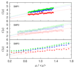
Figure 6: (Color online) Contact number $C(a)$ as a function of particle radius $a$ for two-dimensional packings. The lines correspond to the mean-field approximation of $C(a)$ according to Eq. (9).

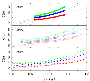
Figure 7: (Color online) The same plots as in Fig. 6, but for three-dimensional packings.

Figure 8: The estimated value of the trace of the average fabric tensor $\phi zg_{{}_{1}}$ vs the exact value $\langle{\mathit{h}}_{{}_{\alpha\alpha}}\rangle_{{}_{V}}$ obtained from the simulations, for several (a) two- and (b) three-dimensional samples. The dashed lines indicate the identity. The insets show more precisely that the deviations increase with $w$, but remain less than $5\%$ in all cases. The symbols are chosen the same as in Table LABEL:Table1.

For comparison with the theory, we first test the validity of assumptions made in Sec. II.3. The linear compacity $c_{s}$ is displayed in Fig. 5 for the static configurations of particles obtained from the isotropic compression simulations. For each particle $p$, the surface angle $\Omega^{{}^{p}}_{c}$ covered by its neighboring particle at contact $c$ is calculated, and the linear compacity of particle $p$ is obtained as $c_{s}^{{}^{p}}{=}\sum_{c=1}^{C_{p}}\Omega^{{}^{p}}_{c}/2\pi$ or $c_{s}^{{}^{p}}{=}\sum_{c=1}^{C_{p}}\Omega^{{}^{p}}_{c}/4\pi$ for two- or three-dimensional packings, respectively. Next, we divide the range of possible values of the particle radius $a$ into $25$ bins. Each data point in Fig. 5 corresponds to the mean value of $c_{s}$, averaged over all particles in the same bin. The contribution of the rattler particles, which transmit no force, is excluded. For moderate widths of size distributions (SMP1), $c_{s}$ is approximately constant in $a$ for a given packing (we note that the fluctuations of $c_{s}$ around its mean value in a given packing originate from the finite size of the samples). However, $c_{s}$ is remarkably above the average value for small particle sizes in wider distributions (SMP2 and SMP3). This is a common property of our highly polydisperse packings (with uniform size distribution) that the fraction of shielded surface is larger than the average for small particles if rattlers are excluded (see Ogarko12 for uniform volume distributions). A similar behavior has been observed in discrete element method simulations of soft particles Goncu10 . There, it is also shown that if rattlers are included in the statistics, the small particles on average are less covered than the larger ones. However, the deviation of small particles from the average $c_{s}$ decreases as the volume fraction of the packing increases by incremental compression.

Another point is that $c_{s}$ depends strongly on the dimension of the system and the friction coefficient. Increasing the friction $\mu_{{}_{f}}$ stabilizes the system in a less dense state and decreases the connectivity of the contact network Kadau03 ; Shaebani09b . Therefore, we expect lower values of $c_{s}$ and $C(a)$ when increasing $\mu_{{}_{f}}$, as confirmed by the data.

In Figs. 6 and 7, the coordination number $C(a)$ is shown as a function of $a$ for the same set of systems as in Fig. 5. For comparison, we also plot $C(a)$ from Eq. (9). Here, the average coordination number $z$ of the packing is taken from the simulation results, $\Omega(a)$ is provided by Eq. (6) or (62), and the size distribution of each packing after the compaction process is used to calculate $q_{{}_{0}}$. The mean-field approach of Sec. II.3 qualitatively fits well to the data, however, the slopes of the curves are slightly greater than the corresponding slopes of the best-fit curves over the data points (not shown). Consequently, one expects that the mean-field approach to calculate the trace of the fabric tensor $\langle{\mathit{h}}_{{}_{\alpha\alpha}}\rangle_{{}_{V}}$ leads to somewhat overestimated values. For each packing, we calculate the exact value of $\langle{\mathit{h}}_{{}_{\alpha\alpha}}\rangle_{{}_{V}}$ via Eq. (4) and compare it with the mean-field approximation [Eq. (10)]. Figure 8 reveals that Eq. (10) slightly overestimates $\langle{\mathit{h}}_{{}_{\alpha\alpha}}\rangle_{{}_{V}}$ in both two- and three-dimensional systems. The deviation increases with the width of the size distribution, but remains less than $5\%$ in all cases. For comparison, note that $g_{{}_{1}}$ can reach up to $1.19$ and $1.45$ in 2D and 3D uniform samples, respectively (see Table LABEL:Table2); therefore, ignoring the correction factor would cause up to $19\%$ and $45\%$ error, respectively.

Table 2: Correction factors in two and three dimensions for uniform size distributions SMP1, SMP2, and SMP3 introduced in Table LABEL:Table1.

sample									$g_{{}_{1}}$									$g_{{}_{2}}$									$g_{{}_{3}}$
SMP1-2D									1.04									1.01									1.04
SMP2-2D									1.12									1.04									1.12
SMP3-2D									1.19									1.07									1.19
SMP1-3D									1.11									1.06									1.005
SMP2-3D									1.30									1.18									1.010
SMP3-3D									1.45									1.30									1.011

Next, we investigate the average properties of the contact force network. In Sec. III.3, we applied the mean-field approach of Sec. II.3 to estimate the isotropic pressure in a given polydisperse granular sample. However, due to the presence of the normal component of the contact force $\bar{F}_{n}(a)$ in Eq. (34), one needs to make one further assumption about the particle-size dependence of $\bar{F}_{n}(a)$ to be able to calculate the integral and obtain $\langle\widetilde{\sigma}_{\alpha\alpha}\rangle_{{}_{V}}$ from the average quantities.

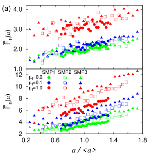
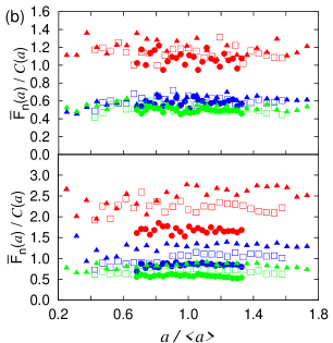
Figure 9: (Color online) (a) Normal component of the contact force $\bar{F}_{n}(a)$, averaged over all particle radii in the same bin, in terms of the particle radius $a$ for two-dimensional (top) and three-dimensional (bottom) packings constructed with different size distribution widths and different friction coefficients $\mu_{{}_{f}}$. (b) $\bar{F}_{n}(a)$ scaled by the contact number $C(a)$ for the same set of samples as in (a).

Figure 10: The estimated value of the trace of the stress tensor using Eq. (76) (top), and Eq. (37) (bottom) divided by $\langle\sigma_{\alpha\alpha}\rangle_{{}_{V}}$ obtained directly from the simulations. Each data point corresponds to a different 2D (top) or 3D (bottom) packing using symbols as in Table LABEL:Table1.

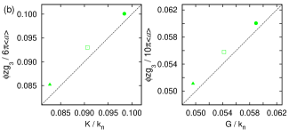
Figure 11: (Color online) The estimated values of the bulk $K$ (left) and shear $G$ (right) moduli according to Eqs. (60) and (61) in 3D [Eqs. (84) and (85) in 2D] vs the values obtained from the simulation results. Each data point corresponds to one frictionless sample and the dashed lines indicate the identity. The results are separately shown for (a) 2D and (b) 3D samples. The same symbols as in Table LABEL:Table1 are used.

The simulation results [Fig. 9(a)] reveal that the average normal force exerted on the particle is an increasing function of the particle radius for 2D and 3D (the contribution of rattlers is again excluded). With increasing friction coefficient and $w$, the average normal force increases. This is reminiscent of the behavior of $C(a)$ as a function of $a$ (Figs. 6 and 7). Interestingly, the increasing rates are similar in both figures. Therefore, it is reasonable to assume that the ratio $\bar{F}_{n}(a)/C(a)$ is independent of $a$, as already observed in 2D Madadi05 . Figure 9(b) confirms the validity of this assumption. We note that the fluctuations in Fig. 9(b) are reduced as the system size increases. In Fig. 10, we compare the exact value of $\langle\sigma_{\alpha\alpha}\rangle_{{}_{V}}$ with the corresponding value from Eq. (37) [or Eq. (76)], which is obtained based on the above assumption. The results are in reasonable agreement with theory for both two- and three-dimensional packings, with a standard deviation of $2\%$ to $6\%$ for increasing $w$.

Finally, we turn to the calculation of the stiffness tensor elements for isotropic materials. We note that to evaluate the true elastic moduli, one should apply an incremental strain and measure the resulting change of the stress tensor. Alternatively, one can read the moduli from the elements of the stiffness tensor, assuming the affine motion of the particles, which cannot be taken for granted however, and which is the subject of future studies. Here, using the packing configuration obtained from the simulation, we calculate the elements of the average stiffness tensor via Eq. (42). Next, the elastic moduli of the packing are calculated using Eqs. (43), (44) and (45). The results are then compared to the estimated values of the bulk and shear moduli calculated via Eqs. (60) and (61) [or Eqs. (84) and (85)]. Figure 11 displays the results for several two- and three-dimensional packings; the agreement is satisfactory within a $5\%$ error (also in the case of frictional packings which is not shown here).

According to our analytical results, the ratio between the bulk and shear moduli $K/G$ is $5/3$ for isotropic packings independent of $z$, $\phi$, and even the size distribution. This suggests that in isotropic packings, the ratio between the $P$-wave velocity $V_{p}{=}\sqrt{(K+\frac{4}{3}G)/\rho}$ and the $S$-wave velocity $V_{s}{=}\sqrt{G/\rho}$ is always $\sqrt{3}$. An experimental test shows that $V_{p}/V_{s}$ for a compressed polydisperse packing of glass beads remains around $1.7$ over a wide range of pressures from $1$ to $7$ MPa Lebedev11 (see also Winkler83 ). Note, however, that anisotropic regular lattice structures do not necessarily show the same ratio Mouraille06 .

VI Discussion and conclusion

In conclusion, a mean-field approach is developed to isolate the influence of size polydispersity on the physical properties of granular assemblies. We are interested in how the microscale quantities are linked to the macroscale ones.

We find that the trace of fabric and stress tensors factorize into the mean packing properties (for example, average coordination number, packing fraction, and average normal contact force) and dimensionless correction factors, which depend on the moments of the particle-size distribution (and approach unity for monodisperse packings). The method is extended to estimate the elements $C_{{}_{\!ijkl}}$ of the stiffness tensor. This tensor describes the linear affine response of the packing to weak external perturbations, when practically the contact network between the particles remains unchanged. The elements $C_{{}_{\!ijkl}}$ are also proportional to the average quantities and a dimensionless correction factor, which is a function of the size distribution.

Numerical simulations illustrate the validity range of our analytical predictions and of the assumptions on which the mean-field method is based. We note that the deviation of the macroscopic quantities of interest from the average packing properties increases with increasing the width $w$ of the particle-size distribution. Figure 12 shows the summarized correction factors $g_{{}_{i}}$ as a function of the width $w$ of a uniform size distribution, with the average particle size $\langle a\rangle$. Neglecting the correction factors would cause remarkable errors, especially for wide distributions. Interestingly, $g_{{}_{3}}$ is insensitive to the width of the size distribution in the 3D case. Therefore, according to Eqs. (60) and (61), we expect that the elastic moduli of a polydisperse packing of spheres is only moderately affected by the choice of $w$. The results of molecular dynamics (MD) simulations of soft frictionless spheres imply (see Eq. (12) in Goncu10 ) that the bulk modulus does not depend on the width of the size distribution, in agreement with our analytical results.

The predictive value of this mean-field method should be examined also by comparing the theoretical predictions with experimental data. For a direct comparison, one needs to measure the average packing properties, e.g. $z$ and $\phi$, which are not easily accessible in experiments (even though microcomputed tomography (MicroCT) scan determines the geometry with micrometer accuracy nowadays Aste05 ). Alternatively, by elimination of $\phi z$ between our analytical results, one obtains linear relationships between the macroscopic physical properties via some coefficients, which depend on the moments of the size distribution. Such linear relations between macroscopic quantities have been investigated in the literature, e.g. between the elastic moduli and conductivity Bristow60 or isotropic pressure Mavko03 , and can be verified experimentally. Future studies will more closely examine the nonaffinity of deformations of isotropic as well as anisotropic packings of frictional and possibly even cohesive particles.

Figure 12: The dimensionless correction factors $g_{{}_{i}}$ in terms of the width $w$ of the uniform size distribution in (a) two and (b) three dimensions. $w/2\langle\displaystyle{a}\rangle\!=\!0$ corresponds to the monodisperse case.

Appendix A Analytical results in two dimensions

Fabric tensor . In a two-dimensional packing of disks [Fig. 13(a)], the surface angle covered by a neighboring particle on the reference particle is

$$\Omega(a)=2\arcsin\Bigg{(}\frac{\langle a\rangle}{a+\langle a\rangle}\Bigg{)},$$ (62)

and the total fraction of the shielded surface is given by

$$c_{s}(a)=\frac{1}{2\pi a}\sum_{i=1}^{C(a)}\Omega(a)a=\Omega(a)C(a)/2\pi.$$ (63)

Assuming that $c_{s}$ is independent of $a$, one can write the mean coordination number $z$ as

$$z=\int_{0}^{\infty}\!\!\!\!C(a)f(a)da=2\pi c_{s}q_{{}_{0}}.$$ (64)

Equations (63) and (64) lead again to Eqs. (9) and (10) for $C(a)$ and $\langle{\mathit{h}}_{{}_{\alpha\alpha}}\rangle_{{}_{V}}$, with the correction factor

$$g_{{}_{1}}=\frac{\displaystyle\int_{0}^{\infty}V(a)\frac{f(a)}{\Omega(a)}da}{q_{{}_{0}}\displaystyle\int_{0}^{\infty}V(a)f(a)da}=\frac{\langle a^{2}\rangle_{{}_{g}}}{\langle a^{2}\rangle}.$$ (65)

By introducing $\epsilon{=}a/\langle a\rangle{-}1$, we rewrite Eq. (62) as

$$\Omega(a)=2\arcsin\Bigg{(}\frac{1}{2+\epsilon}\Bigg{)},$$ (66)

and approximate $1/\Omega(a)$ to the first order in $\epsilon$ for narrow size distributions

$$\frac{1}{\Omega(a)}\simeq A^{\prime}_{{}_{1}}+B^{\prime}_{{}_{1}}\epsilon,$$ (67)

where $\!A^{\prime}_{{}_{1}}\!\!=\!\frac{3}{\pi}$ and $B^{\prime}_{{}_{1}}\!\!=\!\frac{3\sqrt{3}}{\pi^{2}}$. Figure 13(b) reveals that the approximation has a less than $1\%$ error in the range $-0.5\!<\!\epsilon\!<\!1.3$ (or $0.5\langle a\rangle\!<\!a\!<\!2.3\langle a\rangle$). Hence, $g_{{}_{1}}$ for narrow size distributions becomes

$$g_{{}_{1}}\simeq 1+\frac{B^{\prime}_{{}_{1}}}{A^{\prime}_{{}_{1}}}\left(\frac{\big{\langle}\displaystyle{a}^{3}\big{\rangle}}{\big{\langle}\displaystyle{a}\big{\rangle}\big{\langle}\displaystyle{a}^{2}\big{\rangle}}-1\right).$$ (68)

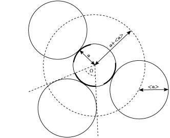
a) b)

Figure 13: (a) A typical particle with radius $a$ surrounded by identical particles of average radius $\langle a\rangle$ in a 2D packing of disks. The thick solid arcs show the shielded surface of the central particle. (b) $1/\Omega(a)$ as a function of $\epsilon$ in two dimensions.

Stress tensor . For a two-dimensional disk, by disregarding the $z$ direction, i.e., in the $x\!-\!y$ plane [by requiring $\theta\!=\!\frac{\pi}{2}$ and $\bar{F}_{t_{1}}^{p}\!\!=\!0$ in Fig. 3(b)], one obtains

$$\widetilde{\sigma}^{p}\!=\frac{a_{p}}{V_{p}}\Biggl{[}\bar{F}_{n}^{p}\sum_{c=1}^{C_{p}}\!\!\left(\begin{array}[]{ccc}\!\!\!\cos^{2}(\varphi)&\!\!\!\!\sin(\varphi)\cos(\varphi)\\ \!\!\!\sin(\varphi)\cos(\varphi)&\!\!\!\!\sin^{2}(\varphi)\end{array}\!\!\!\right)\!\!$$ (71)

$$+\bar{F}_{t_{2}}^{p}\!\!\displaystyle\sum_{c=1}^{C_{p}}\!\!\left(\begin{array}[]{ccc}\!\!\!-\sin(\varphi)\cos(\varphi)&\!\!\!\!\cos^{2}(\varphi)\\ \!\!\!-\sin^{2}(\varphi)&\!\!\!\!\sin(\varphi)\cos(\varphi)\end{array}\;\!\!\!\right)\Biggr{]},$$ (74)

and its trace

$$\widetilde{\sigma}^{{}^{p}}_{{}_{\alpha\alpha}}=\frac{a_{p}}{V_{p}}\sum_{c=1}^{C_{p}}\sum_{\alpha=1}^{D}\biggl{(}\bar{F}_{n}^{p}\;n^{{}^{pc}}_{\alpha}n^{{}^{pc}}_{\alpha}+\bar{F}_{t_{2}}^{p}\;n^{{}^{pc}}_{\alpha}t_{2\alpha}^{{}^{pc}}\biggr{)}$$ (75)

$${=}\displaystyle\frac{a_{p}}{V_{p}}\!\!\displaystyle\sum_{c=1}^{C_{p}}\biggl{(}\!\!\bar{F}_{n}^{p}|\hat{n}^{{}^{pc}}\!|^{{}^{2}}{+}\bar{F}_{t_{2}}^{p}\hat{n}^{{}^{pc}}\!\!\!\!\cdot\hat{t}_{2}^{{}^{pc}}\!\!\biggr{)}{=}\frac{a_{p}}{V_{p}}\bar{F}_{n}^{p}C_{p}.$$

Using Eqs. (34) and (36), the average stress tensor in 2D becomes

$$\langle\widetilde{\sigma}_{{}_{\alpha\alpha}}\rangle_{{}_{V}}=\displaystyle\frac{\phi z\;\bar{F}_{n}(\langle\displaystyle{a}\rangle)\;g_{{}_{2}}}{\pi\big{\langle}\displaystyle{a}\big{\rangle}},$$ (76)

with

$$g_{{}_{2}}=\displaystyle\frac{\pi\langle\displaystyle{a}\rangle\displaystyle\int_{0}^{\infty}\!\!\!\displaystyle{a}\frac{f(\displaystyle{a})}{\Omega^{2}(\displaystyle{a})}\,d\displaystyle{a}}{3q_{{}_{0}}\langle\displaystyle{a}^{2}\rangle}.$$ (77)

By Taylor expansion around $\epsilon\!\!\!=\!\!0$, we approximate $1/\Omega^{2}(a)$ as

$$\frac{1}{\Omega^{2}(a)}\simeq A^{\prime}_{{}_{2}}+B^{\prime}_{{}_{2}}\epsilon,$$ (78)

with $\!A^{\prime}_{{}_{2}}\!\!=\!A^{\prime^{{}^{2}}}_{{}_{1}}\!\!=\!\displaystyle\frac{9}{\pi^{2}}$ and $B^{\prime}_{{}_{2}}\!\!=\!\displaystyle\frac{18\sqrt{3}}{\pi^{3}}$. Therefore, $g_{{}_{2}}$ can be approximated by

$$g_{{}_{2}}\simeq\frac{B^{\prime}_{{}_{2}}}{A^{\prime}_{{}_{2}}}+\big{(}1{-}\frac{B^{\prime}_{{}_{2}}}{A^{\prime}_{{}_{2}}}\big{)}\frac{\big{\langle}\displaystyle{a}\big{\rangle}^{2}}{\big{\langle}\displaystyle{a}^{2}\big{\rangle}}.$$ (79)

Stiffness tensor . Similarly to the three-dimensional analysis presented in Sec. IV, we approximate the summation over neighbors in Eq. (46) by $\frac{C(a)}{2\pi}\int_{{}_{0}}^{{}^{2\pi}}n_{\alpha}n_{\beta}n_{\gamma}n_{\eta}d\theta$, which leads to the following reduced stiffness tensor (by mapping $11\rightarrow 1$, $22\rightarrow 2$ and $12\rightarrow 3$):

$$\langle\mathcal{C}\rangle_{{}_{V}}=\frac{\phi zk_{n}g_{{}_{3}}}{4\pi}\left(\begin{array}[]{cccc}3&1&0\\ &3&0\\ &&1\end{array}\right),$$ (80)

with

$$g_{{}_{3}}(=g_{{}_{1}})=\langle\displaystyle{a}^{2}\rangle_{{}_{g}}/\langle\displaystyle{a}^{2}\rangle,$$ (81)

which for narrow size distributions is approximated as

$$g_{{}_{3}}\simeq 1+\frac{B^{\prime}_{{}_{1}}}{A^{\prime}_{{}_{1}}}\left(\frac{\big{\langle}\displaystyle{a}^{3}\big{\rangle}}{\big{\langle}\displaystyle{a}\big{\rangle}\big{\langle}\displaystyle{a}^{2}\big{\rangle}}-1\right).$$ (82)

In two dimensions, one finds that the Lamé constants for frictionless isotropic packings are

$$\mu=\lambda=(k_{n}\phi zg_{{}_{3}})\,/\,(4\pi),$$ (83)

and, hence, the shear and bulk moduli are

$$G/k_{n}=(\phi zg_{{}_{3}})\,/\,(4\pi),$$ (84)

and

$$K/k_{n}=(\phi zg_{{}_{3}})\,/\,(2\pi).$$ (85)

References

- (1) P. G. de Gennes, Rev. Mod. Phys. 71, 374 (1999).
- (2) H. M. Jaeger, S. R. Nagel, and R. P. Behringer, Rev. Mod. Phys. 68, 1259 (1996).
- (3) H. Hinrichsen and D. E. Wolf, The Physics of Granular Media (Wiley-VCH, Weinheim, 2004).
- (4) F. Radjai, M. Jean, J. J. Moreau, and S. Roux, Phys. Rev. Lett. 77, 274 (1996).
- (5) H. A. Makse, D. L. Johnson, and L. M. Schwartz, Phys. Rev. Lett. 84, 4160 (2000).
- (6) S. Ostojic and D. Panja, Phys. Rev. Lett. 97, 208001 (2006).
- (7) S. Luding, Int. J. Solids Struct. 41, 5821 (2004).
- (8) M. Wackenhut, S. McNamara, and H. Herrmann, Eur. Phys. J. E 17, 237 (2005).
- (9) C. Voivret, F. Radjai, J.-Y. Delenne, and M. S. El Youssoufi, Phys. Rev. Lett. 102, 178001 (2009).
- (10) H. J. Herrmann, R. Mahmoodi Baram, and M. Wackenhut, Physica A 330, 77 (2003).
- (11) C. Voivret, F. Radjai, J.-Y. Delenne, and M. S. El Youssoufi, Phys. Rev. E 76, 021301 (2007).
- (12) P.S. Dodds and J. S. Weitz, Phys. Rev. E 65, 056108 (2002).
- (13) V. Ogarko and S. Luding, submitted to J. Chem. Phys. (2011).
- (14) M. Madadi, O. Tsoungui, M. Lätzel, and S. Luding, Int. J. Solids Struct. 41, 2563 (2004).
- (15) J. J. Moreau, Eur. J. Mech. A/Solids 13, 93 (1994).
- (16) M. Jean, Comput. Methods Appl. Mech. Eng. 177, 235 (1999).
- (17) L. Brendel, T. Unger, and D. E. Wolf, The Physics of Granular Media (Wiley-VCH, Weinheim, 2004) pp 325-343.
- (18) M. R. Shaebani, T. Unger, and J. Kertész, Int. J. Mod. Phys. C 20, 847 (2009).
- (19) J. D. Goddard, Recent Developments in Structured Continua. Pitman Research Notes in Mathematics No. 143 (Longman, New York, 1986) p 179.
- (20) C. S. Chang, Micromechanics of Granular Materials (Elsevier, Amsterdam, 1988) pp 271-279.
- (21) L. Rothenburg and A.P.S. Selvadurai, Mechanics of Structured Media (Elsevier, Amsterdam, 1981) pp 469-486; M. M. Mehrabadi, S. Nemat-Nasser, H. M. Shodja, and G. Subhash, 1988 Micromechanics of Granular Materials (Elsevier, Amsterdam, 1988) pp 253-262; M. H. Sadd, J. Gao, and A. Shukla, Comput. Geotech. 20, 323 (1997); J. D. Goddard, Physics of Dry Granular Media (Kluwer Academic Publishers, Dordrecht, 1998) pp 1-24; C. S. Chang, S. J. Choa, and Y. Chang, Int. J. Solids Struct. 32, 1989 (1995).
- (22) M. M. Mehrabadi, S. Nemat-Nasser, and M. Oda, Int. J. Numer. Anal. Meth. Geomech. 6, 95 (1982).
- (23) M. Lätzel, S. Luding, and H. J. Herrmann, Granular Matter 2, 123 (2000).
- (24) S. C. Cowin, Mech. Mater. 4, 137 (1985); A. M. Sadegh, S. C. Cowin, and G. M. Lou, Mech. Mater. 11, 323 (1991); P. Dubujet and F. Dedecker, Granular Matter 1, 129 (1998); S. C. Cowin, J. Biomech. 31, 759 (1998); D. Bigoni and B. Loret, J. Mech. Phys. Solids 47, 1409 (1999).
- (25) O. Durán, N. P. Kruyt, and S. Luding, Int. J. Solids Struct. 47, 251 (2010); O. Durán, N. P. Kruyt, and S. Luding, Int. J. Solids Struct. 47, 2234 (2010).
- (26) N. Ouchiyama and T. Tanaka, Ind. Eng. Chem. Fundam. 20, 66 (1981).
- (27) J. Christoffersen, M. M. Mehrabadi, and S. Nemat-Nasser, J. Appl. Mech. 48, 339 (1981).
- (28) M. Madadi, S. M. Peyghoon, and S. Luding, Powders and Grains (Balkema, Leiden, 2005) pp 93-97.
- (29) N. P. Kruyt and L. Rothenburg, J. Appl. Mech. 118, 706 (1996).
- (30) M. R. Shaebani, J. Boberski, and D. E. Wolf, submitted to Granular Matter (2011).
- (31) O. Mouraille, W. A. Mulder, and S. Luding, J. Stat. Mech. P07023 (2006).
- (32) R. J. Bathurst and L. Rothenburg, J. Appl. Mech. 55, 17 (1988).
- (33) H. C. Andersen, J. Chem. Phys. 72, 2384 (1980).
- (34) F. Göncü, O. Durán, and S. Luding, C. R. Mecanique 338, 570 (2010).
- (35) D. Kadau, G. Bartels, L. Brendel, and D. E. Wolf, Phase Trans. 76, 315 (2007).
- (36) M. R. Shaebani, T. Unger, and J. Kertész, Phys. Rev. E 79, 052302 (2009).
- (37) M. Lebedev, Rock Physics Lab, Curtin University, 2011 (private communication).
- (38) K. W. Winkler, Geophys. Res. Lett. 10, 1073 (1983).
- (39) T. Aste, M. Saadatfar, and T. J. Senden, Phys. Rev. E 71, 061302 (2005).
- (40) J. R. Bristow, Br. J. Appl. Phys. 11, 81 (1960).
- (41) G. Mavko, T. Mukerji, and J. Dvorkin, The Rock Physics Handbook (Cambridge University Press, Cambridge, 2003).