Magic-zero wavelengths of alkali-metal atoms and their applications

Abstract

Using first-principles calculations, we identify “magic-zero” optical wavelengths, $\lambda_{\rm{zero}}$, for which the ground-state frequency-dependent polarizabilities of alkali-metal atoms vanish. Our approach uses high-precision, relativistic all-order methods in which all single, double, and partial triple excitations of the Dirac-Fock wave functions are included to all orders of perturbation theory. We discuss the use of magic-zero wavelengths for sympathetic cooling in two-species mixtures of alkalis with group-II and other elements of interest. Special cases in which these wavelengths coincide with strong resonance transitions in a target system are identified.

I Introduction

The realization of mixtures of trapped ultracold atomic gases  Truscott et al. (2001); Schreck et al. (2001a); Modugno et al. (2001); Ivanov et al. (2011); Baumer et al. (2011) has opened new paths towards the formation of ultracold diatomic molecules Papp and Wieman (2006); Ospelkaus et al. (2006); Ospelkaus and Ospelkaus (2008); Ni et al. (2008); Voigt et al. (2009), quantum-state control of chemical reactions Ospelkaus et al. (2010), prospects for quantum computing with polar molecules DeMille (2002); Micheli et al. (2006); Carr et al. (2009), tests of fundamental symmetries Hudson et al. (2002); Shafer-Ray (2006); Meyer and Bohn (2009) and studies of fundamental aspects of correlated many-body systems Tassy et al. (2010), and dilute quantum degenerate systems Hadzibabic et al. (2002a); Roati et al. (2002); Regal et al. (2004); Chin et al. (2004); Kinast et al. (2004). Co-trapped diamagnetic-paramagnetic mixtures have also made possible experimental realization of interspecies Feshbach resonances Stan et al. (2004); Inouye et al. (2004); Naik et al. (2011), two-species Bose-Einstein condensates and mixed Bose-Fermi and Fermi-Fermi degenerate gases Schreck et al. (2001b); Hadzibabic et al. (2002b); Modugno et al. (2002); Tassy et al. (2010).

In an optical lattice, atoms can be trapped in the intensity maxima or minima of the light field by the optical dipole force Grimm et al. (2000). This force arises from the dispersive interaction of the induced atomic dipole moment with the intensity gradient of the light field, and is proportional to the ac polarizability of the atom. When its ac polarizability vanishes, as can happen at certain wavelengths, an atom experiences no dipole force and thus is unaffected by the presence of an optical lattice. Our present work provides accurate predictions of the “magic-zero wavelengths” $\lambda_{\rm{zero}}$ which lead to zero Stark shifts for alkali-metal atoms. These wavelengths have also been designated as “tune-out wavelengths” by LeBlanc and Thywissen Leblanc and Thywissen (2007).

We suggest some possible uses for such wavelengths, all of which take advantage of the fact (demonstrated below), that magic-zero wavelengths are highly dependent upon atomic species and state. For a given atomic species and state A, let ${\rm L}_{\rm{A}}$ designate an optical lattice or trap made with light at one of the magic-zero wavelengths of A. We start with a model configuration consisting of the gas A embedded in ${\rm L}_{\rm{A}}$ and confined by another trap, T. Some process is performed on the gas, after which T is turned off. Members of A will depart and ${\rm L}_{\rm{A}}$ may confine whatever is left. For example, one might photoassociate some A atoms into dimers during the initial period, and thereby be left with a nearly pure population of dimers trapped in ${\rm L}_{\rm{A}}$ at the end. LeBlanc and Thywissen Leblanc and Thywissen (2007) have pointed out the advantage of magic-zero wavelengths for traps containing two species. If another species, B, is added to the model configuration, it will ordinarily be affected by ${\rm L}_{\rm{A}}$, so B can be moved by shifting ${\rm L}_{\rm{A}}$, while A remains unaffected. Schemes of this type have been used for entropy transfer and controlled collisions between ⁸⁷Rb and ⁴¹K Catani et al. (2009); Lamporesi et al. (2010); McKay and DeMarco (2011). For bichromatic optical lattice schemes, such as those discussed by Brickman Soderberg, et al. Brickman Soderberg et al. (2009); Klinger et al. (2010), it could be useful to incorporate ${\rm L}_{\rm{B}}$ into the model configuration, so as to be able to move A and B completely independently. In another application, a Sr lattice at a ³P₀ magic-zero wavelength was suggested for realization of quantum information processing Daley et al. (2008).

In the next section, we briefly discuss the calculation of frequency-dependent polarizabilities of alkali-metal atoms. In section III, we present the magic-zero wavelengths for the alkalis from Li to Cs and discuss some of their applications.

II Frequency-dependent polarizabilities

The background to our approach to calculation of atomic polarizabilities is treated in a recent review article Mitroy et al. (2010). Here we summarize points salient to the present work. The frequency-dependent scalar polarizability, $\alpha^{v}_{0}(\omega)$, of an alkali-metal atom in its ground state $v$ may be separated into a contribution from the core electrons, $\alpha_{\rm{core}}$, a core modification due to the valence electron, $\alpha_{vc}$, and a contribution from the valence electron, $\alpha_{v}(\omega)$. Since core electrons have excitation energies in the far-ultraviolet region of the spectrum, the core polarizability dependends weakly on $\omega$ for the optical frequencies treated here. Therefore, we approximate the core polarizability by its dc value as calculated in the random-phase approximation (RPA)  Johnson et al. (1983), an approach that has been quite successful in previous applications. The core polarizability is corrected for Pauli blocking of core-valence excitations by introducing an extra term $\alpha_{vc}$. For consistency, this is also calculated in RPA. Therefore, the ground state polarizability may be separated as

$$\alpha_{0}(\omega)=\alpha_{\rm{core}}+\alpha_{vc}+\alpha_{0}^{v}(\omega).$$ (1)

The valence contribution to the static ac polarizability is calculated using the sum-over-states approach Safronova and Clark (2004):

$$\alpha_{0}^{v}(\omega)=\frac{2}{3(2j_{v}+1)}\sum_{k}\frac{{\left\langle k\left\|D\right\|v\right\rangle}^{2}(E_{k}-E_{v})}{(E_{k}-E_{v})^{2}-\omega^{2}},$$ (2)

where $\left\langle k\left\|D\right\|v\right\rangle$ is the reduced electric-dipole (E1) matrix element. In this equation, $\omega$ is assumed to be at least several linewidths off resonance with the corresponding transitions. Unless stated otherwise, we use the conventional system of atomic units, a.u., in which $e,m_{\rm e}$, $4\pi\epsilon_{0}$ and the reduced Planck constant $\hbar$ have the numerical value 1. Polarizability in a.u. has the dimension of volume, and its numerical values presented here are expressed in units of $a^{3}_{0}$, where $a_{0}\approx 0.052918$ nm is the Bohr radius. The atomic units for $\alpha$ can be converted to SI units via $\alpha/h$ [Hz/(V/m)²]=2.48832$\times 10^{-8}\alpha$ [a.u.], where the conversion coefficient is $4\pi\epsilon_{0}a^{3}_{0}/h$ and the Planck constant $h$ is factored out.

Table 1: $5s-np$ contributions to the frequency-dependent polarizability of the ground state of Rb at $\lambda_{\textrm{zero}}=423.0448$ nm = 1/(23638.16 cm^-1). Absolute values of electric-dipole matrix elements are expressed in a.u. ($ea_{0}$), and the corresponding energy differences are expressed in conventional wavenumber units (cm^-1 ).

Contribution	$|\langle 5s\|D\|np_{1/2}\rangle|$	$E_{np_{j}}-E_{5s}$	$\alpha_{0}$
$5p_{1/2}$	4.231	12579.0	-41.130
$6p_{1/2}$	0.325	23715.1	50.235
$7p_{1/2}$	0.115	27835.0	0.124
$8p_{1/2}$	0.059	29835.0	0.023
$np_{1/2}$ tail			0.085
$5p_{3/2}$	5.978	12816.5	-84.938
$6p_{3/2}$	0.528	23792.6	66.140
$7p_{3/2}$	0.202	27870.1	0.383
$8p_{3/2}$	0.111	29853.8	0.081
$np_{3/2}$ tail			0.285
$\alpha_{\textrm{core}}$			9.076
$\alpha_{vc}$			-0.367
$\alpha_{0}^{v}$			-8.712
Total $\alpha_{0}(\omega)$			0.00

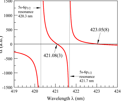
Figure 1: The frequency-dependent polarizability of the Rb ground state. The first two zero-magic wavelengths are marked with arrows.

Table 2: Magic-zero wavelengths $\lambda_{\rm{zero}}$ for alkali-metal atoms from Li to Cs. The resonant wavelengths $\lambda_{\rm{res}}$ for relevant transitions are also listed. The wavelengths (in vacuum) are given in nm.

Atom	Resonance	$\lambda_{\rm{res}}$	$\lambda_{\rm{zero}}$
6Li	$2s-2p_{1/2}$	670.992478
			670.987445(1)
	$2s-2p_{3/2}$	670.977380
7Li	$2s-2p_{1/2}$	670.976658
			670.971626(1)
	$2s-2p_{3/2}$	670.961561
Li			324.18(6)
	$2s-3p_{1/2}$	323.3576
	$2s-3p_{3/2}$	323.3566
			274.911(7)
	$2s-4p_{1/2}$	274.2001
Na	$3s-3p_{1/2}$	589.7558
			589.5565(3)
	$3s-3p_{3/2}$	589.1583
			331.905(3)
	$3s-4p_{1/2}$	330.3929
			330.3723
	$3s-4p_{3/2}$	330.3319
			285.5817(8)
	$3s-5p_{1/2}$	285.3850
K	$4s-4p_{1/2}$	770.1083
			768.971(3)
	$4s-4p_{3/2}$	766.7009
			405.98(4)
	$4s-5p_{1/2}$	404.8356
			404.72(4)
	$4s-5p_{3/2}$	404.5285
			344.933(1)
	$4s-6p_{1/2}$	344.8363
Rb	$5s-5p_{1/2}$	794.9789
			790.034(7)
	$5s-5p_{3/2}$	780.2415
			423.05(8)
	$5s-6p_{1/2}$	421.6726
			421.08(3)
	$5s-6p_{3/2}$	420.2989
			359.42(3)
	$5s-7p_{1/2}$	359.2593
Cs	$6s-6p_{1/2}$	894.5929
			880.25(4)
	$6s-6p_{3/2}$	852.3472
			460.22(2)
	$6s-7p_{1/2}$	459.4459
			457.31(3)
	$6s-7p_{3/2}$	455.6557
			389.029(4)
	$6s-8p_{1/2}$	388.9714

The calculation of the ground state frequency-dependent polarizabilities in alkali-metal atoms has been previously discussed in  Safronova et al. (2006); Arora et al. (2007), and we give only brief summary of the approach. The sum over intermediate $k$ states in Eq. (2) converges rapidly. Therefore, we separate the valence state polarizability into two parts, $\alpha_{\rm{main}}$, containing the contributions from the few lowest $np$ states, and the remainder, $\alpha_{\rm{tail}}$. We note that our calculations are carried out with the finite basis set constructed using B-splines Johnson et al. (1988) making the sum finite. In the calculation of $\alpha_{\rm{main}}$, we use the experimental values compiled in Ref. Safronova et al. (1999) along with their uncertainties for the first $ns-np$ matrix elements, for example the $4s-4p_{j}$ matrix elements in K. For all other terms, we use the relativistic all-order values  Safronova and Johnson (2007); Safronova et al. (1999) of the matrix elements and the experimental values of the energies NIS (a); Moore (1971); NIS (b). In the relativistic all-order method, all single-double (SD) or single-double and partial valence triple (SDpT) excitations of the Dirac-Fock (DF) wave function are included to all orders of perturbation theory Safronova et al. (1999); Blundell et al. (1991); Safronova and Clark (2004). We conduct additional semi-empirical scaling of our all-order values (SD_sc) where we expect scaled values to be more accurate or for more accurate evaluation of the uncertainties. Our scaling procedure and evaluation of the uncertainties of the all-order results have been recently discussed in Ref. Safronova and Safronova (2011). Briefly, the uncertainties of the all-order matrix elements are given by the spread of their SD, SDpT, SD_sc and SDpT_sc values. These are also used to calculate the uncertainties in the state-by-state contributions to the frequency-dependent polarizability. The tail contributions, $\alpha_{\rm{tail}}$, are calculated in the DF approximation using complete basis set functions that are linear combinations of B-splines Safronova et al. (2004). In the cases treated here, the tail contribution is of the order of 1% of the net valence contribution $\alpha_{0}^{v}$.

We define the magic-zero wavelength $\lambda_{\rm{zero}}$ as the wavelength where the ac polarizability of the ground state vanishes. In practice, we calculated $\alpha_{0}(\omega)$ for a range of values in the vicinity of relevant resonances and identified values of $\omega$ where the polarizability turned to zero with sufficient numerical accuracy.

Table 3: Wavelength (in vacuum) of selected transitions in Mg, Ca, Zn, Cd, Sr, Ba, Hg, Yb, Dy, Ho, and Er in nm.

Atom	Transition	Wavelength	Transition	Wavelength
Mg	$3s^{2}~{}^{1}S_{0}-3s3p~{}^{1}P_{1}$	285.3	$3s^{2}\ {}^{1}S_{0}-3s3p\ ^{3}P_{1}$	457.2
Ca	$4s^{2}~{}^{1}S_{0}-4s4p~{}^{1}P_{1}$	422.8	$4s^{2}\ {}^{1}S_{0}-4s4p\ ^{3}P_{1}$	657.5
Sr	$5s^{2}~{}^{1}S_{0}-5s5p~{}^{1}P_{1}$	460.9	$5s^{2}\ {}^{1}S_{0}-5s5p\ ^{3}P_{1}$	689.5
Ba	$6s^{2}~{}^{1}S_{0}-6s6p~{}^{1}P_{1}$	553.7	$6s^{2}\ {}^{1}S_{0}-6s6p\ ^{3}P_{1}$	791.4
Zn	$4s^{2}~{}^{1}S_{0}-4s4p~{}^{1}P_{1}$	213.9	$4s^{2}\ {}^{1}S_{0}-4s4p\ ^{3}P_{1}$	307.7
Cd	$5s^{2}~{}^{1}S_{0}-5s5p~{}^{1}P_{1}$	228.9	$5s^{2}\ {}^{1}S_{0}-5s5p\ ^{3}P_{1}$	326.2
Hg	$6s^{2}~{}^{1}S_{0}-6s6p~{}^{1}P_{1}$	184.9	$6s^{2}\ {}^{1}S_{0}-6s6p\ ^{3}P_{1}$	253.7
Yb	$6s^{2}~{}^{1}S_{0}-6s6p~{}^{1}P_{1}$	398.9	$6s^{2}\ {}^{1}S_{0}-6s6p\ ^{3}P_{1}$	555.8
Dy	$4f^{10}6s^{2}\ {}^{5}I_{8}-4f^{10}(^{5}I_{8})~{}6s6p~{}(^{1}P_{1})$ $J=9$	421.3
Er	$4f^{12}6s^{2}\ {}^{3}H_{6}-4f^{11}(^{3}H_{6})~{}6s6p~{}(^{3}P_{1})$ $J=7$	582.8
Ho	$4f^{11}6s^{2}\ {}^{4}I_{15/2}-4f^{11}(^{4}I_{15/2})~{}6s6p~{}(^{3}P_{1})$ $J=17/2$	598.5
Ho	$4f^{11}6s^{2}\ {}^{4}I_{15/2}-4f^{11}(^{4}I_{15/2})~{}6s6p~{}(^{1}P_{1})$ $J=13/2$	416.4

We illustrate the cancellation of all contributions to $5s$ Rb polarizability at $\lambda_{\rm{zero}}$=423.0448 nm in Table 1. Since this wavelength is between $5s-5p_{3/2}$ and $5s-6p_{1/2}$ resonances, the contributions of the $5p_{j}$ and $6p_{j}$ terms strongly dominate. However, the contribution from the core is significant (11% of the largest valence term). This table shows that $\lambda_{\rm{zero}}$ is located where the valence contribution to the polarizability cancels the adjusted core contribution, a feature that is common to all the cases treated here. The zero crossing point is in the close vicinity of the $5s-6p_{1/2}$ resonance owing to the relative size of the $5s-5p_{j}$ and $5s-6p_{j}$ reduced electric-dipole matrix elements given in the second column of Table 1. The $5s-6p$ matrix elements are more than an order of magnitude smaller than the $5s-5p$ matrix elements. Since polarizability contributions are proportional to the square of the matrix element, the denominators of the $6p_{j}$ terms have to become very small to cancel out the $5p$ contributions.

This magic-zero wavelength is illustrated in Fig. 1 where we plot ground-state polarizability of Rb atom in a.u. in the vicinity of the $5s-6p_{j}$ resonances. Another zero crossing point shown in the figure is located between $5s-6p_{1/2}$ and $5s-6p_{3/2}$ resonances, as expected. The next magic-zero wavelength will be located close to the $5s-7p_{1/2}$ resonance since the values of the matrix elements continue to decrease with $n$.

III Results and Applications

In Table 2, we list the vacuum $\lambda_{\rm{zero}}$ wavelengths for alkali-metal atoms from Li to Cs. For convenience of presentation, we also list the resonant wavelength $\lambda_{\rm{res}}$ in vacuum in the relevant range of wavelengths. We order the lists of the resonant wavelengths and $\lambda_{\rm{zero}}$ to indicate the respective placements of $\lambda_{\rm{zero}}$ and their distances from resonances. The resonant vacuum wavelength values are obtained from energy levels from National Institute of Standards and Technology (NIST) database NIS (a) with the exception of the $2s-2p_{1/2}$ and $2s-2p_{3/2}$ transition wavelengths for ⁶Li and ⁷Li that are taken from recent measurements Sansonetti et al. (2011).

Since alkali ground states have electric dipole transitions only to $p$ states, their polarizabilities will cross zero only between two $ns-n^{\prime}p$ resonances. We set the wavelength of the $ns-(n+2)p_{1/2}$ resonance as a lower wavelength bound for our search. The fine structure of the $(n+2)p$ level is sufficiently small for all alkalis to make the zero point between $ns-(n+2)p_{1/2}$ and $ns-(n+2)p_{3/2}$ relatively difficult to use in practice, so we do not list it. We omit the $\lambda_{\rm{zero}}$ between $2s-3p_{j}$ resonances for the same reason. The wavelengths of the next zero-crossing near the $ns-(n+3)p_{1/2}$ resonances are in the ultraviolet, and not as readily accessible in most laboratories, so we have not calculated them. However, this would be a routine matter for future work. There are no $\lambda_{\rm{zero}}$ at wavelengths greater than those of the primary $ns-np_{1/2}$ resonances. Within these constraints, we have found four $\lambda_{\rm{zero}}$ for Na, K, Rb, and Cs and three $\lambda_{\rm{zero}}$ for Li, as shown in Table 1.

The stated uncertainties in the $\lambda_{\rm{zero}}$ values are taken to be the maximum difference between the central value and the crossing of the $\alpha_{{0}}\pm\delta\alpha_{0}$ with zero, where $\delta\alpha_{0}$ is the uncertainty in the ground state polarizability value at that wavelength. The uncertainties in the values of polarizabilities are obtained by adding uncertainties in the individual polarizability contributions in quadrature.

We find small but significant differences in the first magic wavelengths of ⁶Li and ⁷Li due to the isotope shift. These values refer to the centers of gravity of all hyperfine states and do not take into account the hyperfine structure. Therefore, this $\lambda_{\rm{zero}}$ and the corresponding $2s-2p_{j}$ resonance wavelengths are listed separately. We verified that isotope shift of the $2s-2p$ traditions in Li does not affect the next magic wavelength, 324.18(6)nm, so we use NIST data for the other transitions. We also investigated possible dependence of the first magic-zero wavelengths on the isotope shift for ³⁹K, ⁴⁰K, ⁴¹K and ⁸⁵Rb, ⁸⁷Rb. The D1 ($4s-4p_{1/2}$) and D2 ($4s-4p_{3/2}$) line wavelengths for ³⁹K, ⁴⁰K, and ⁴¹K have been measured using a femtosecond laser frequency comb by Falke et al. Falke et al. (2006). We carry out three calculations of the first magic-zero wavelength using D1, D2 wavelengths for the specific isotope in our calculations. The resulting value for ³⁹K and ⁴⁰K, 768.971(3)nm, is the same as the value quoted in Table 2. The ⁴¹K value is 768.970(3)nm, with the difference being well below our quoted uncertainty. The calculations of the first magic wavelength in Rb using D1 and D2 frequencies for ⁸⁵Rb and ⁸⁷Rb listed in Steck (a, b) gave results identical to result from Table 2, 790.034(7)nm that was obtained using NIST data. We note that our values for the first magic wavelengths are in good agreement with LeBlanc and Thywissen Leblanc and Thywissen (2007) calculations with the exception of their value for ⁴⁰K.

The first magic-zero wavelength in Rb has been measured to be 789.85(1)nm in Catani et al. (2009). Some discrepancy with our result is most likely due to approximate linear polarization of the beam in Catani et al. (2009). The difference is compatible with a shift in the magic zero wavelength caused by few percent spurious $\sigma^{-}$ polarization component com .

Below, we identify two main applications of magic-zero wavelengths. First, these wavelengths are advantageous for cooling of group-II and other more complicated atoms, by sympathetic cooling using an accompanying alkali atom.

Recently, group II atoms have been the subject of various experiments and proposals in atomic clock research and quantum information. BEC of ⁸⁴Sr has been reported recently by two groups Stellmer et al. (2009); Desalvo et al. (2010). The element Yb has four boson and two fermion isotopes, all of which have been cooled into the microkelvin range. Several exciting new prospects for quantum information processing with the ground state nuclear spin have recently been identified in group II elements Daley et al. (2008). Also, Sr or Yb are useful for polarized mixtures of fermions, or Bose-Fermi mixtures, where isotopic mixtures can be studied.

More complex systems have become of interest in the development of frequency standards and quantum information processing schemes. For example, the rare earth holmium is a candidate for quantum information applications Saffman and Mølmer (2008) due to its rich ground-state hyperfine structure. Erbium has been a subject of recent experimental work McClelland and Hanssen (2006); Berglund et al. (2007), stimulated by its possible use in a variety of applications, including narrow linewidth laser cooling and spectroscopy, unique collision studies, and degenerate bosonic and fermionic gases with long-range magnetic dipole coupling.

Some species, particularly fermions, are difficult to cool by themselves due to unfavorable ultracold collisional dynamics. In such cases, it may be possible to use sympathetic cooling in a mixture of the target species and one of the alkalis, where the alkali-metal atom is cooled directly by standard techniques. This has recently been demonstrated in Yb:Rb mixtures Tassy et al. (2010). Use of $\lambda_{\rm{zero}}$ trap wavelengths could allow one to release alkali atoms after the target atoms of the other species are sufficiently cold, in a hybrid trap configuration that combines optical and magnetic traps or bichromatic optical traps. If the final trap configuration utilizes a $\lambda_{\rm{zero}}$ wavelength, strong trapping of the target atom is possible while alkali atoms will be released by turning off its separate trapping potential. Since placement of the resonances varies significantly among the alkali-metal atoms, a wide range of $\lambda_{\rm{zero}}$ is available as shown in Table 3.

We list the resonant wavelengths for variety of atomic systems in Table 3. For consistency with the other tables, we list vacuum wavelengths obtained from the NIST energy levels database NIS (b). Comparing Tables 2 and 3 yields many instances of resonant transitions that are very close to $\lambda_{\rm{zero}}$. Here are few of the very close cases: Mg 285.3 - Na 285.6, Sr 460.9 - Cs 460.2, Dy 421.3 - Rb 421.1, Ho 598.5 - Na 589.6.

Magic-zero wavelength laser light may be also useful in three-species cooling schemes such as reported in Ref. Taglieber et al. (2008) by allowing easy release of one of the species from the trap. The work Taglieber et al. (2008) demonstrated that the efficiency of sympathetic cooling of the ⁶Li gas by ⁸⁷Rb was increased by the presence of ⁴⁰K through catalytic cooling.

Measurements of the magic-zero wavelengths may be used as high-precision benchmark tests of theory and determination of the excited-state matrix elements that are difficult to measure by other methods. Matrix elements of $ns-n^{\prime}p$ transitions of alkali-metal atoms, where $ns$ is the ground state, are difficult to calculate accurately owing to large correlation corrections and small values of the final numbers. Experimental measurements of the $\lambda_{\rm{}_{zero}}$ predicted in this work will serve an an excellent benchmark test of the all-order calculations. Moreover, it will be possible to combine these measurements with theoretical calculations to infer the values of these small matrix elements. Only one high-precision measurement of such matrix elements ($6s-7p_{j}$ transitions in Cs) has been carried out to date  Vasilyev et al. (2002).

IV conclusion

In summary, we calculate magic-zero wavelengths in alkali-metal atoms from Li to Cs and estimate their uncertainties. Applications of these magic wavelengths to sympathetic cooling of group-II and other more complicated atoms with alkalis are discussed. Special cases where these wavelengths coincide with strong resonance transition in group-II atoms, Yb, Dy, Ho, and Er are identified. Measurements of the magic-zero wavelengths for benchmark tests of theory and experiment are proposed.

This research was performed under the sponsorship of the US Department of Commerce, National Institute of Standards and Technology, and was supported by the National Science Foundation under Physics Frontiers Center Grant PHY-0822671. This work was performed in part under the sponsorship of the Department of Science and Technology, India. We thank Joseph Reader and Craig Sansonetti for helpful discussions.

References

- Truscott et al. (2001) A. G. Truscott, K. E. Strecker, W. I. McAlexander, G. B. Partridge, and R. G. Hulet, Science 291, 2570 (2001).
- Schreck et al. (2001a) F. Schreck, L. Khaykovich, K. L. Corwin, G. Ferrari, T. Bourdel, J. Cubizolles, and C. Salomon, Phys. Rev. Lett. 87, 080403 (2001a).
- Modugno et al. (2001) G. Modugno, G. Ferrari, G. Roati, R. J. Brecha, A. Simoni, and M. Inguscio, Science 294, 1320 (2001).
- Ivanov et al. (2011) V. V. Ivanov, A. Khramov, A. H. Hansen, W. H. Dowd, F. Muenchow, A. O. Jamison, and S. Gupta, Phys. Rev. Lett. 106, 153201 (2011).
- Baumer et al. (2011) F. Baumer, F. Münchow, A. Görlitz, S. E. Maxwell, P. S. Julienne, and E. Tiesinga, ArXiv e-prints (2011), eprint 1104.1722.
- Papp and Wieman (2006) S. B. Papp and C. E. Wieman, Phys. Rev. Lett. 97, 180404 (2006).
- Ospelkaus et al. (2006) C. Ospelkaus, S. Ospelkaus, L. Humbert, P. Ernst, K. Sengstock, and K. Bongs, Phys. Rev. Lett. 97, 120402 (2006).
- Ospelkaus and Ospelkaus (2008) C. Ospelkaus and S. Ospelkaus, J. Phys. B 41, 203001 (2008).
- Ni et al. (2008) K.-K. Ni, S. Ospelkaus, M. H. G. de Miranda, A. Pe’er, B. Neyenhuis, J. J. Zirbel, S. Kotochigova, P. S. Julienne, D. S. Jin, and J. Ye, Science 322, 231 (2008).
- Voigt et al. (2009) A.-C. Voigt, M. Taglieber, L. Costa, T. Aoki, W. Wieser, T. W. Hänsch, and K. Dieckmann, Phys. Rev. Lett. 102, 020405 (2009).
- Ospelkaus et al. (2010) S. Ospelkaus, K.-K. Ni, D. Wang, M. H. G. de Miranda, B. Neyenhuis, G. Quemener, P. S. Julienne, J. L. Bohn, D. S. Jin, and J. Ye, Science 327, 853 (2010).
- DeMille (2002) D. DeMille, Phys. Rev. Lett. 88, 067901 (2002).
- Micheli et al. (2006) A. Micheli, G. K. Brennen, and P. Zoller, Nature Physics 2, 341 (2006).
- Carr et al. (2009) L. D. Carr, D. DeMille, R. V. Krems, and J. Ye, New Journal of Physics 11, 055049 (2009).
- Hudson et al. (2002) J. J. Hudson, B. E. Sauer, M. R. Tarbutt, and E. A. Hinds, Phys. Rev. Lett. 89, 023003 (2002).
- Shafer-Ray (2006) N. E. Shafer-Ray, Rhys. Rev. A 73, 034102 (2006).
- Meyer and Bohn (2009) E. R. Meyer and J. L. Bohn, Phys. Rev. A 80, 042508 (2009).
- Tassy et al. (2010) S. Tassy, N. Nemitz, F. Baumer, C. Höhl, A. Batär, and A. Görlitz, J. Phys. B 43, 205309 (2010).
- Hadzibabic et al. (2002a) Z. Hadzibabic, C. A. Stan, K. Dieckmann, S. Gupta, M. W. Zwierlein, A. Görlitz, and W. Ketterle, Phys. Rev. Lett. 88, 160401 (2002a).
- Roati et al. (2002) G. Roati, F. Riboli, G. Modugno, and M. Inguscio, Phys. Rev. Lett. 89, 150403 (2002).
- Regal et al. (2004) C. A. Regal, M. Greiner, and D. S. Jin, Phys. Rev. Lett. 92, 040403 (2004).
- Chin et al. (2004) C. Chin, M. Bartenstein, A. Altmeyer, S. Riedl, S. Jochim, J. H. Denschlag, and R. Grimm, Science 305, 1128 (2004).
- Kinast et al. (2004) J. Kinast, S. L. Hemmer, M. E. Gehm, A. Turlapov, and J. E. Thomas, Phys. Rev. Lett. 92, 150402 (2004).
- Stan et al. (2004) C. A. Stan, M. W. Zwierlein, C. H. Schunck, S. M. Raupach, and W. Ketterle, Phys. Rev. Lett. 93, 143001 (2004).
- Inouye et al. (2004) S. Inouye, J. Goldwin, M. L. Olsen, C. Ticknor, J. L. Bohn, and D. S. Jin, Phys. Rev. Lett. 93, 183201 (2004).
- Naik et al. (2011) D. Naik, A. Trenkwalder, C. Kohstall, F. M. Spiegelhalder, M. Zaccanti, G. Hendl, F. Schreck, R. Grimm, T. M. Hanna, and P. S. Julienne (2011), Eur. Phys. J. D, DOI: 10.1140/epjd/e2010-10591-2.
- Schreck et al. (2001b) F. Schreck, L. Khaykovich, K. L. Corwin, G. Ferrari, T. Bourdel, J. Cubizolles, and C. Salomon, Phys. Rev. Lett. 87, 080403 (2001b).
- Hadzibabic et al. (2002b) Z. Hadzibabic, C. A. Stan, K. Dieckmann, S. Gupta, M. W. Zwierlein, A. Görlitz, and W. Ketterle, Phys. Rev. Lett. 88, 160401 (2002b).
- Modugno et al. (2002) G. Modugno, G. Roati, F. Riboli, F. Ferlaino, R. J. Brecha, and M. Inguscio, Science 297, 2240 (2002).
- Grimm et al. (2000) R. Grimm, M. Weidemuller, and Y. B. Ovchinnikov, Adv. At. Mol. Opt. Phys. 42 (2000).
- Leblanc and Thywissen (2007) L. J. Leblanc and J. H. Thywissen, Phys. Rev. A 75, 053612 (2007).
- Catani et al. (2009) J. Catani, G. Barontini, G. Lamporesi, F. Rabatti, G. Thalhammer, F. Minardi, S. Stringari, and M. Inguscio, Phys. Rev. Lett. 103, 140401 (2009).
- Lamporesi et al. (2010) G. Lamporesi, J. Catani, G. Barontini, Y. Nishida, M. Inguscio, and F. Minardi, Phys. Rev. Lett. 104, 153202 (2010).
- McKay and DeMarco (2011) D. C. McKay and B. DeMarco, Rep. Prog. Phys. 74, 054401 (2011).
- Brickman Soderberg et al. (2009) K. Brickman Soderberg, N. Gemelke, and C. Chin, New J. Phys. 11, 055022 (2009).
- Klinger et al. (2010) A. Klinger, S. Degenkolb, N. Gemelke, K.-A. B. Soderberg, and C. Chin, Review of Scientific Instruments 81, 013109 (2010).
- Daley et al. (2008) A. J. Daley, M. M. Boyd, J. Ye, and P. Zoller, Phys. Rev. Lett. 101, 170504 (2008).
- Mitroy et al. (2010) J. Mitroy, M. S. Safronova, and C. W. Clark, J. Phys. B 43, 202001 (2010).
- Johnson et al. (1983) W. R. Johnson, D. Kolb, and K.-N. Huang, At. Data Nucl. Data Tables 28, 334 (1983).
- Safronova and Clark (2004) M. S. Safronova and C. W. Clark, Phys. Rev. A 69, 040501(R) (2004).
- Safronova et al. (2006) M. S. Safronova, B. Arora, and C. W. Clark, Phys. Rev. A 73, 022505 (2006).
- Arora et al. (2007) B. Arora, M. S. Safronova, and C. W. Clark, Phys. Rev. A. 76, 052509 (2007).
- Johnson et al. (1988) W. R. Johnson, S. A. Blundell, and J. Sapirstein, Phys. Rev. A 37, 307 (1988).
- Safronova et al. (1999) M. S. Safronova, W. R. Johnson, and A. Derevianko, Phys. Rev. A 60, 4476 (1999).
- Safronova and Johnson (2007) M. S. Safronova and W. R. Johnson, Adv. At. Mol. Opt. Phys. 55, 191 (2007).
- NIS (a) Yu. Ralchenko and A. E. Kramida and J. Reader and NIST ASD Team, NIST Atomic Spectra Database (version 4.0). [Online]. Available: http://physics.nist.gov/asd. National Institute of Standards and Technology, Gaithersburg, MD.
- Moore (1971) C. E. Moore, Atomic Energy Levels, vol. 35 of Natl. Bur. Stand. Ref. Data Ser. (U.S. Govt. Print. Off., 1971).
- NIS (b) J. E. Sansonetti and W. C. Martin and S. L. Young, Handbook of Basic Atomic Spectroscopic Data (version 1.1.2). [Online] Available: http://physics.nist.gov/Handbook. (2005) National Institute of Standards and Technology, Gaithersburg, MD.
- Blundell et al. (1991) S. A. Blundell, W. R. Johnson, and J. Sapirstein, Phys. Rev. A 43, 3407 (1991).
- Safronova and Safronova (2011) M. S. Safronova and U. I. Safronova, Phys. Rev. A 83, 012503 (2011).
- Safronova et al. (2004) M. S. Safronova, C. J. Williams, and C. W. Clark, Phys. Rev. A 69, 022509 (2004).
- Sansonetti et al. (2011) C. J. Sansonetti, C. E. Simien, J. D. Gillaspy, J. N. Tan, S. M. Brewer, R. C. Brown, S. Wu, and J. V. Porto, Phys. Rev. Lett. 107, 023001 (2011).
- Falke et al. (2006) S. Falke, E. Tiemann, C. Lisdat, H. Schnatz, and G. Grosche, Phys. Rev. A 74, 032503 (2006).
- Steck (a) D. A. Steck, rubidium 85 D Line Data,” available online at http://steck.us/alkalidata (revision 2.1.4, 23 December 2010).
- Steck (b) D. A. Steck, rubidium 87 D Line Data,” available online at http://steck.us/alkalidata (revision 2.1.4, 23 December 2010).
- (56) Francesco Minardi, private communication.
- Stellmer et al. (2009) S. Stellmer, M. K. Tey, B. Huang, R. Grimm, and F. Schreck, Phys. Rev. Lett. 103, 200401 (2009).
- Desalvo et al. (2010) B. J. Desalvo, M. Yan, P. G. Mickelson, Y. N. Martinez de Escobar, and T. C. Killian, Phys. Rev. Lett. 105, 030402 (2010).
- Saffman and Mølmer (2008) M. Saffman and K. Mølmer, Phys. Rev. A 78, 012336 (2008).
- McClelland and Hanssen (2006) J. J. McClelland and J. L. Hanssen, Phys. Rev. Lett. 96, 143005 (2006).
- Berglund et al. (2007) A. J. Berglund, S. A. Lee, and J. J. McClelland, Phys. Rev. A 76, 053418 (2007).
- Tassy et al. (2010) S. Tassy, N. Nemitz, F. Baumer, C. Höhl, A. Batär, and A. Görlitz, J. Phys. B: At. Mol. Opt. Phys. 43, 205309 (2010).
- Taglieber et al. (2008) M. Taglieber, A. Voigt, T. Aoki, T. W. Hänsch, and K. Dieckmann, Phys. Rev. Lett. 100, 010401 (2008).
- Vasilyev et al. (2002) A. A. Vasilyev, I. M. Savukov, M. S. Safronova, and H. G. Berry, Phys. Rev. A 66, 020101 (2002).