Deep Multiwaveband Observations of the Jets of 0208–512 and 1202–262

Abstract

We present deep HST, Chandra, VLA and ATCA images of the jets of PKS 0208–512 and PKS 1202–262, which were found in a Chandra survey of a flux-limited sample of flat-spectrum radio quasars with jets (see Marshall et al., 2005). We discuss in detail their X-ray morphologies and spectra. We find optical emission from one knot in the jet of PKS 1202–262 and two regions in the jet of PKS 0208–512. The X-ray emission of both jets is most consistent with external Comptonization of cosmic microwave background photons by particles within the jet, while the optical emission is most consistent with the synchrotron process. We model the emission from the jet in this context and discuss implications for jet emission models, including magnetic field and beaming parameters.

1. Introduction

Relativistic jets appear to be a common result of accretion onto compact objects. The jets of active galactic nuclei (AGN) include objects with a wide range of luminosities and sizes. In the most powerful sources – quasars and Fanaroff-Riley type II (FR II, Fanaroff & Riley 1974) radio galaxies – the jets terminate at the hot spots, compact bright regions hundreds of kpc away from the nucleus of the host galaxy, where the jet flow collides with the intergalactic medium (IGM), inflating the radio lobes. AGN jets are enormously powerful, with a total bolometric power output that is often comparable to or greater than that from the host galaxy, and a kinetic energy flux that can be comparable to the AGN’s bolometric luminosity (Rawlings & Saunders 1991).

Until the last decade, almost all progress towards understanding the physics of jets had come either from numerical modeling or multi-frequency radio mapping. However, the pace of discovery has accelerated greatly in the past decade with HST and Chandra observations. One of the first observations by Chandra is a perfect illustration: the target, PKS 0637–752, was a bright radio-loud quasar. It was believed that this source would be unresolved in the X-rays, and therefore ideally suited to focus the telescope. Instead, we saw a beautiful X-ray jet well over 10 arcseconds long (Chartas et al. 2000, Schwartz et al. 2000), with morphology similar to that seen in the radio. Deeper multi-band observations of this jet have since been done to constrain the nature of its emission and also its matter/energy content (Georganopoulos et al. 2005, Uchiyama et al. 2005, Mehta et al. 2009). Indeed, since the launch of the two Great Observatories, the number of extended, arcsecond-scale jets known to emit in the optical and X-rays has increased about ten-fold, from less than 5 to more than 50, including members of every luminosity and morphological class of radio-loud AGN.

For jets, multiwaveband observations give physical constraints that cannot be gained in any other way. In the bands where synchrotron radiation is the likely emission mechanism (for the most part, radio through optical), one can combine images to derive information regarding particle acceleration, jet orientation, kinematics and dynamics, electron spectrum and other information. The X-ray emission mechanism can be either synchrotron (with very short particle lifetimes) or inverse-Compton in nature (for recent reviews, see Harris & Krawczynski 2006, Worrall 2009). In either case, the X-ray emission gives a new set of constraints on jet physics, because it represents either (in the case of synchrotron radiation) the most energetic particles ($\gamma\sim 10^{6}-10^{8}$) in the jet, which must be accelerated in situ, or (in the case of inverse-Compton emission) the very lowest energy ($\gamma\sim$ few - hundreds) particles, a population that controls the jet’s matter/energy budget yet cannot be probed by any other observations, and which still must be linked to the low-frequency radio emission. Combining information in multiple bands can then give unique information on the magnetic field and beaming parameters as well as the matter/energy budget of the jet.

Following the discovery of bright X-ray emission from the jet in PKS 0637–752, we embarked on a survey (Marshall et al. 2005, hereafter Paper I) to assess the rate of occurrence and properties of X-ray jets among the population of quasars. Our initial goals were to assess the level of detectable X-ray fluxes from radio-bright jets, to locate good targets for detailed imaging and spectral followup studies, and where possible to test models of the X-ray emission by measuring the broad-band, spatially resolved, spectral energy distributions (SED) of jets from the radio through the optical to the X-ray band. The survey has been largely successful in achieving these aims, thanks to a relatively high success rate of about 60% of the first 39 observed (Marshall et al., 2011).

We have used the survey data ($\sim 5$ ks Chandra observations) along with other multiwavelength data (including both longer Chandra observations as well as deep observations in other bands) to study the spectral energy distributions and jet physics of several of the jets in our sample (Gelbord et al. 2005; Schwartz et al. 2006a (hereafter Paper II), 2006b, 2007; Godfrey et al. 2009). Here we discuss relatively deep (35-55 ks) Chandra and HST (2–3 orbits) observations of PKS B0208–512 and PKS B1202–262 (hereafter 0208–512 and 1202–262 respectively), two of the X-ray brightest jets found in our survey. Both had 40-115 counts detected in the initial Chandra survey observation, which detected multiple jet emission regions in the X-rays as well as make an initial assessment of the jet physics (Paper II). The goal of these deeper observations was to examine these conditions in greater detail, assess the jet’s morphology and spectral energy distribution in multiple bands, and constrain the X-ray spectrum and emission mechanism.

0208–512 and 1202–262 were first discovered in the Parkes Survey of Radio Sources (Bolton et al. 1964). 0208–512 was first identified by Peterson et al. (1979) as a quasar at $z=1.003$, and is a powerful X-ray and Gamma-ray emitter. It was one of the first extragalactic sources detected by both EGRET (Bertsch et al. 1993) and COMPTEL (Blom et al. 1995), and has highly unusual gamma-ray properties, being one of the few blazars characterized by flares at MeV energies, rather than in the GeV or TeV domains (Stacy et al. 1996, Blom et al. 1996). 1202–262 was identified as a quasar by Wills, Wills & Douglas (1973) and Peterson et al. (1979). It is at a redshift of $z=0.789$.

In §2 we discuss the observations and data reduction procedures, while in §3, we discuss results from these observations. In §4, we present a discussion of physical constraints that can be gained from these observations. Finally, in §5, we sum up our conclusions. Henceforth, we use a flat, accelerating cosmology, with $H_{0}=71{\rm km~{}s^{-1}~{}Mpc^{-1}}$ (for consistency with Paper II), $\Omega_{M}=0.27$ and $\Omega_{\Lambda}=0.73$.

2. Observations and Data Reduction

2.1. Chandra Observations

Deep Chandra observations were obtained for both of our target sources, using the ACIS-S in FAINT mode. Chandra observed 0208–512 on 20 February 2004 for a total integration time of 53.66 ks, using a standard 1/8 subarray and a frame time of 0.4 seconds. The Chandra observations of 1202–262 were obtained 26 November 2004 for a total integration time of 39.17 ks, using a standard 1/4 subarray and a frame time of 0.8 seconds. The choices of subarray and frame time were driven by the core fluxes (Paper I), with the goal of avoiding pileup greater than 10%. Roll angle ranges were requested to keep the jet more than 30^∘ from a readout streak.

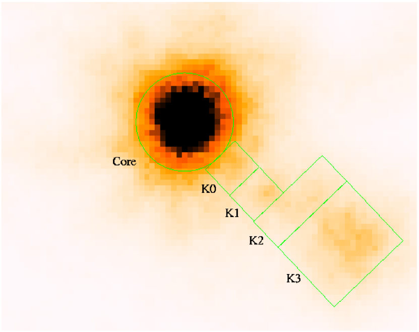
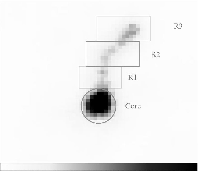
Figure 1.— Our deep Chandra observations of 0208–512. Outlined in green are the core and four jet regions used for photometry. This image was sub-sampled to a resolution of 0.2 times the native ACIS-S pixel size (i.e., 0.0984^′′/pix) and adaptively smoothed with a minimum of 10 counts per ellipse. Three knot regions are clearly resolved from the nucleus (K1, K2, K3), while a fourth region (K0) that is seen in the F814W HST observations is possibly resolved from the nucleus.

Figure 2.— Our deep Chandra observations of 1202–262. Outlined in green are the core and three jet regions used for photometry. This image was sub-sampled to a resolution of 0.5 times the native ACIS-S pixel size (i.e., 0.246^′′/pix) and adaptively smoothed with a minimum of 10 counts per ellipse. The morphology of this jet is quite smooth, although a significant brightening is seen towards the terminus of the X-ray bright region. No change in surface brightness is seen as the jet bends gently through about 50 degrees.

The images were reduced in CIAO using standard recipes. This included the derandomization of photon positions within pixels, destreaking, filtering out flare-affected portions and bad pixels, as well as resampling images to 0.2 and 0.5 times the native ACIS pixel size (respectively 0$\farcs$092 and 0$\farcs$246 per pixel). When the data filtering was completed, the effective exposure times for the two observations were 48.67 ks for 0208–512 and 30.01ks for 1202–262. All photons between 0.3-10 keV were used for both image and spectral analysis. The resulting Chandra image of 0208–512 is shown in Figure 1, while the Chandra image of 1202–262 is shown in Figure 2.

2.2. HST Observations

We also obtained HST observations for both sources. We used the ACS/WFC and obtained images in both the F814W and F475W bands. We requested roll angles to keep the jet at least 30 degrees from a diffraction spike. Our observing strategy was optimized both for long integrations as well as to obtain a high-quality PSF for the central QSO. This involved a combination of both long exposures (on which the central pixels are saturated) and short exposures, with the latter serving to fix the properties of the quasar PSF. We CR-SPLIT and dithered each observation by integral pixel amounts to minimize the impact of bad pixels and cosmic rays. In order to minimize the readout time we also limited the WFC field of view to a 1024 $\times$ 1024 section of chip 1 (point position WFC1-1K). Our HST observations of 0208–512 took place on 26-27 May 2004 for three orbits. The total exposure time in the F814W band was 3240s for the deep exposures and 340s for the shallow exposures, while in the F475W band our integration times were 3114s for the deep exposures and 140s for the shallow exposures. The HST observations of 1202–262 took place on 9 June 2004 for two orbits. The total integration time in the F475W band was 1980s for the deep exposure and 100s for the shallow exposure, while in the F814W band the total integration times were 2088s for the deep exposure and 100s for the shallow exposure.

One of our objects (0208–512) was also observed on 10 July 2004 for 2 orbits by the HST/ACS in the same bands by another team (led by F. Tavecchio), using a substantially simpler strategy. In particular, they did not obtain short exposures to measure the PSF, nor did they dither to eliminate bad pixels. Moreover, as described in their paper (Tavecchio et al. 2007), in those data the jet fell on a diffraction spike because the roll angle was not specified. Because Tavecchio et al. also ended up using our data for their analysis, we will refer to their paper when discussing any differences between our findings and theirs for this source.

All HST data were reduced in IRAF and PyRAF using standard recipes. The data were drizzled onto a common grid using MultiDrizzle (Koekemoer et al. 2002 and references therein). As part of the drizzling process, the images were rotated to a north-up, east-left configuration. Since no sub-pixel drizzling was done, we did not subsample, hence leaving the data at the native ACS/WFC pixel size of 0$\farcs$05 per pixel. All observations were used to obtain the final summed image, with weights awarded according to their exposure time. We also used MultiDrizzle to sum the shorter exposures to obtain the QSO’s fluxes and compare the PSF with that generated by TinyTim (see next paragraph).

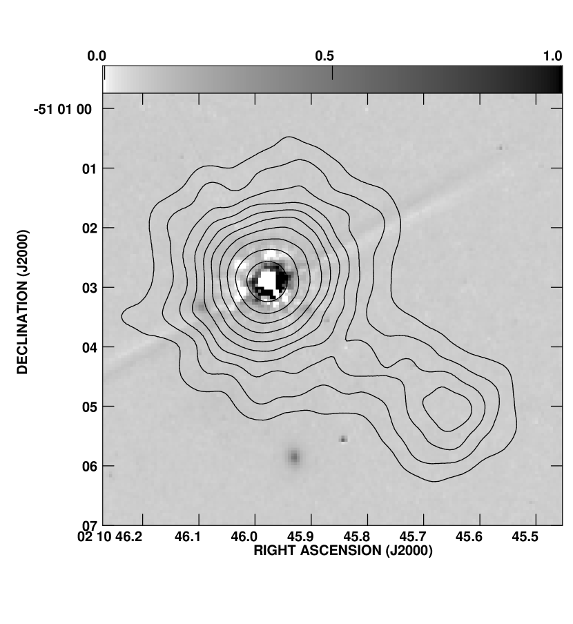
Figure 3.— Our HST images of 0208–512 (greyscales) with Chandra X-ray contours overlaid. At top, we show the F814W image, while at bottom we show the F475W image. The Chandra image has been convolved with a $0.3^{\prime\prime}$ Gaussian. A scaled, TinyTim PSF has been used to subtract out the quasar point source in the optical. We have convolved the F814W image with a $0.2^{\prime\prime}$ Gaussian to better show the possible optical counterparts to knots K0 and K3, which are particularly faint. Some evidence of oversubtraction is seen at the center of the quasar; however, this is unavoidable given that the quasar is saturated and given the general problem of charge bleed. The contours are at (2, 4, 6, 8 …) photons per pixel. See text for details.

TinyTim simulations (Krist & Burrows 1994, Suchkov & Krist 1998, Krist & Hook 2004) were obtained for PSF subtraction in both bands. For the TinyTim simulations we assumed an optical spectrum of the form $F_{\nu}\propto\nu^{-1}$. Previous experience with TinyTim has shown that the PSF shape is not heavily dependent on spectral slope. Separate TinyTim simulations were performed for each observation. The most difficult part of the PSF subtraction was correctly normalizing and rotating the PSF. This necessitated independent rotation of each of the two axes to north-up (as the two axes of the WFC detector are not completely orthogonal on the sky), as well as iteratively looking at residuals and attempting to minimize the diffraction spikes. Importantly, because the charge ’bleed’ in ACS data is linear, the total flux of a saturated object is preserved even when heavy saturation is observed. Thus, in these data, we optimized the PSF models for the subtraction of the outer isophotes, comparing to the short exposures for the overall normalization. Because the long exposures were saturated, this also inevitably led to negatives in the central pixels; however, given the small residuals in other places plus the relatively smooth off-jet isophotes, we believe the result is reliable.

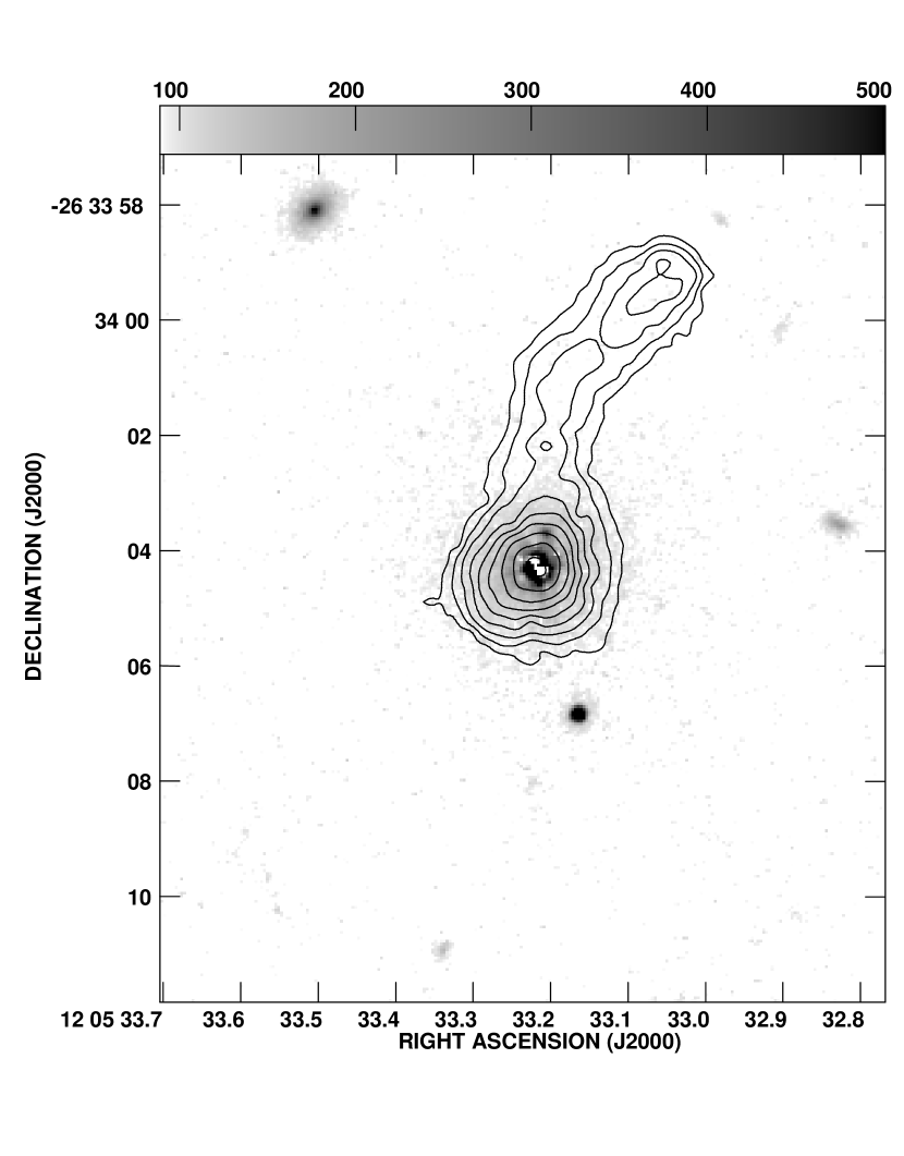
Figure 4.— Our HST images of 1202–262 (greyscales), with Chandra X-ray contours overlaid. The pixellation and smoothing is as in the previous figures. At top, we show the F814W image, and at bottom, we show the F475W image. The contours are at (2, 4, 6, 8 …) photons per pixel. In both, a TinyTim PSF has been used to subtract out optical emission from the quasar. As with 0208–512’s HST images, there is some evidence of oversubtraction, but the problem is less severe for this object since its quasar point source is less bright. Both images show an object $0.4^{\prime\prime}$ NNW of the quasar. This object is quite blue (see text for discussion) and likely associated with a jet knot.

2.3. Radio Observations

The radio observations used in this paper were obtained at both the Australia Telescope Compact Array (ATCA) and NRAO Very Large Array (VLA). In Paper I we presented ATCA observations of both sources at 8.6 GHz. In addition to those data we also obtained 4.8 GHz VLA observations of 1202$-$262 as well as 20.1 GHz ATCA observations of both sources.

The 4.8 GHz VLA data were obtained in the A configuration on 5 November 2000 as part of project AM0672. The 8.6 GHz ATCA data were obtained in May and September 2000 for 1202$-$262 and February 2002 for 0208$-$512. Observations were made in two array configurations, 6 km and 1.5 km to provide high angular resolution imaging ($\sim$1.2 arcsec) as well as good sensitivity to extended structures. The 20.1 GHz data from the ATCA presented here were collected as part of a high-angular resolution radio-wavelength followup, complementary to the deeper Chandra and HST observations. These new ATCA observations were made with the array in a 6 km (6C) configuration, providing an angular resolution of  0.5 arcsec FWHM, well matched to the Chandra PSF. The 20.1 GHz observations of 0208$-$512 and 1202$-$262 were carried out on 2004 May 8 and 2004 May 13 respectively.

Both sources were observed in full polarization at a bandwidth of 128 MHz. The sources were typically observed in groups of two or three with scans of 10 minutes duration interleaved over a 12 hour period. At 8.6 GHz, 0208$-$512 was observed for a total of 310 minutes and 1202$-$262 was observed for 440 minutes. At 20.1 GHz, 0208$-$512 was observed for a total of 250 minutes and 1202$-$262 was observed for 290 minutes. The primary calibrator 1934$-$638 was observed and flux densities of 2.842 Jy and 0.923 Jy were assumed at 8.64 and 20.1 GHz respectively. Short $\sim 1$ min scans of nearby compact secondary calibrators were scheduled for the two program sources to provide initial phase and gain calibration.

The ATCA data were calibrated in MIRIAD (Sault, Teuben & Wright 1995) using the standard reduction path for continuum data and, imaging was carried out with Difmap (Shepherd 1997), where phase and amplitude self-calibration were applied. The images shown here were made using uniform weighting and restored with a circular beam of equal area to the FWHM of the true synthesized beam. The VLA data were reduced using standard procedures in AIPS.

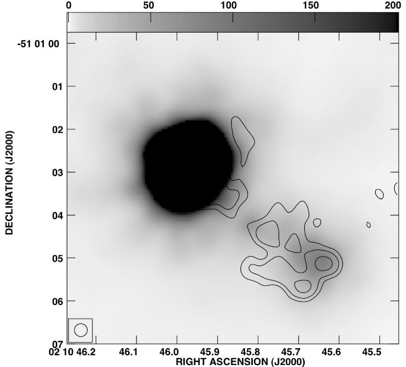
Figure 5.— Our Chandra image of 0208–512 (greyscale, with smoothing and pixellation as in Figure 3) with radio contours overlaid. The radio contours are taken from our new 20.1 GHz ATCA data and have a restoring beam size of 0.44 arcsec. The contours are at (1, 2, 4, 8 …) $\times$ 0.5 mJy/beam. Note that the radio and X-ray morphologies are somewhat different; in particular the maxima of K1 and K2 are not at the same locations, and the southeastern part of knot K3 appears somewhat brighter in the radio (relative to the northwestern part) than in the X-rays. See text for discussion.

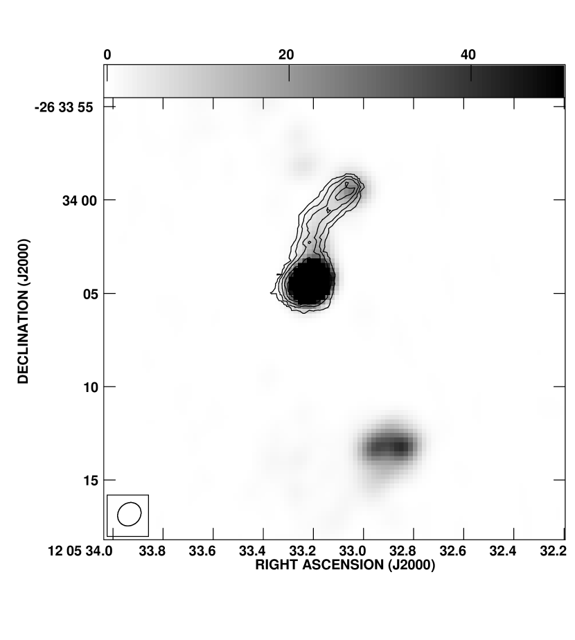
Figure 6.— Our ATCA 8.6 GHz image of 1202–262 (greyscale), with Chandra X-ray contours overlaid. As can be seen, the X-ray emission from the jet has a morphology similar to that seen in the radio. No X-ray emission is seen from the region beyond the sharp bend, or from the counterjet side.

2.4. Cross-Registration

Images were registered to one another assuming identical nuclear positions in all bands. As the absolute positional information in HST images is set by the guide star system and is typically only accurate to $1^{\prime\prime}$, the radio images were used as the fiducial, adhering to the usual IAU standard. All other images were therefore registered to the VLA image. Following this, the $1\sigma$ errors in the positions from the HST images should be $\pm 0.2^{\prime\prime}$ in RA and DEC (see e.g., Deutsch 1999), while the absolute errors in the X-ray image are $\pm 0.4^{\prime\prime}$, relative to either the radio or optical. The relative errors, however, should be closer to $0.1^{\prime\prime}$, as long as the assumption is correct that the quasar is the brightest source in each band. Armed with this information, we were then able to produce overlays of optical, radio and X-ray images.

In Figure 3, we show the deep HST images of 0208–512, while in Figure 4, we show the deep HST images of 1202–262. Both figures show contours made from the Chandra images overlaid. In Figure 5 and 6 respectively, we show overlays of radio contours onto the Chandra image of 0208–512 and 1202–262. In Figures 7 and 8, we show radio/optical overlays of each object. Finally, in Figure 9, we show the run of jet brightness with distance for both objects, in both the 20 GHz radio images and the X-ray images. To produce the plots in Figure 9 we used the FUNTOOLS ”counts in regions” task, to produce radial profiles for each quasar plus jet and the quasar only. This allowed us to produce PSF-subtracted profiles, useful for revealing structure in the inner 1-2 arcseconds.

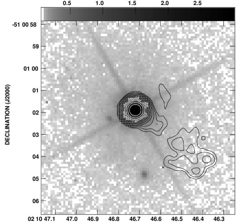
Figure 7.— Our F814W HST image of 0208–512 (greyscale) with radio contours from our 20 GHz ATCA image overlaid. This figure shows the likely link between the optical sources within the jet contours and jet components K0 and K3. See text for discussion.

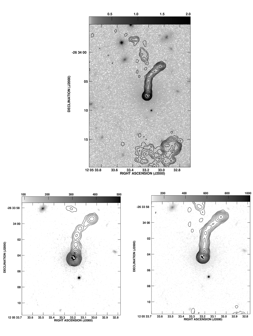
Figure 8.— Three views of 1202–262 showing the HST F814W image (greyscale) overlaid with radio contours. At top, we show a broader view, with contours from the 4.8 GHz VLA A-array image. As can be seen, no optical sources can be firmly associated with any jet structure, with the exception of the source $0.4^{\prime\prime}$ north of the quasar. At bottom, we zoom in on the X-ray bright region of the jet, using the same region plotted in previous figures. The left panel shows the 20 GHz ATCA contours, while the right-hand panel shows the same 4.8 GHz VLA A-array image shown in the top panel. The 20 GHz ATCA image has a restoring beam size of 0.59 arcsec. These plots cement the identification of the optical source at $0.4^{\prime\prime}$ with a jet knot. In addition, we see that the morphology of the jet changes quite significantly with frequency in the radio band, with the higher-frequency map showing a much knottier jet that is quite different from what is seen in X-rays. The smoother morphology seen at lower frequency is much more similar to the Chandra image.

Figure 9.— Radial profiles for both the 0208–512 and 1202–262 jet. The solid line indicates the X-ray flux while the dotted line indicates the radio profiles. Note the significant differences between the radio and X-ray morphologies of both jets. See text for discussion.

3. Results

3.1. PKS B0208–512

The radio structure of 0208–512 is complex, and extends $5^{\prime\prime}$ SW of the core, with the innermost parts significantly more compact than the rather diffuse outer component. There is possible evidence of a 90^∘ bend in the 8.6 GHz ATCA maps given in Paper I; however, the higher-resolution 20 GHz image (contours shown in Figure 5) shows the bend only at low significance. VLBI and VSOP observations (Tingay et al. 1996, Shen et al. 1998, Tingay et al. 2002) show a milliarcsecond-scale jet at a position angle similar to that seen on arcsecond scales. Given the lack of lower-frequency radio data for this source at subarcsecond resolution, we did not attempt to make a radio spectral index map for 0208–512. The X-ray structure of this source, as described by Paper II, has two, possibly three emission regions, which were labeled R1, R2 and R3 (the last labelled with a question mark due to the detection of only seven counts) in that paper. As shown in Figures 1, 3, 5 and 7, however, our deeper observation shows the X-ray, radio and optical structure of this source to be somewhat more complex. We identify a total of four knot regions in the jet, which we have labelled K0, K1, K2 and K3, in increasing order of distance from the nucleus. There is also a possible extension of the nuclear source seen in the F475W image (Figure 3) only; however, it is not fully resolved, and could also be an artifact of the undersampling of the PSF combined with the location of the quasar within the central pixel. We therefore do not attempt to measure quantities associated with this source.

The relationship of K0-K3 to the emission regions described by Paper II is complex. Region K0 lies closer to (distance 0$\farcs$8 from) the nucleus than any of the regions pointed out by Paper II, and is not well resolved from the nucleus in the X-rays. It is, however, easily resolved from the nucleus in radio and appears to have a faint optical counterpart (Figures 3 and 5). When the point source is subtracted from both the radio and X-ray images in a radial profile (Figure 9), K0 is seen more clearly at distances of 0.7-1.5 arcseconds from the nucleus. The data contain tempting hints of a significant morphology difference between the radio and X-ray in K0, as the flux peak is located closer to the nucleus in the radio than the X-ray. However, the errors in the X-ray point source subtraction are large enough to make this not definitive. K1 corresponds roughly to the region labelled R1 by Paper II; hence the name, chosen to minimize confusion. This region is the faintest in radio and X-rays. There is faint optical emission in this region; however, there is nothing that stands out above the level of the galaxy. Therefore, we do not believe this jet region has significant optical emission connected with it.

The region labelled R2 in Paper II is seen to split into two fairly distinct maxima, which we have here called K2 and K3. K2 is seen easily in the radio as well but any optical emission lies below our detectability threshold. It should be noted, however, that the sole radio maximum in the region of K1 and K2 actually lies in between these knots. It is therefore unclear whether these represent knots in the physical sense. K3 appears to have a rather complex structure. In the radio, two distinct peaks are seen along with a component on the south side that appears to extend back towards the nucleus. The X-ray emission appears to come from the entire region but is brighter on the north side. The comparison of radio and X-ray flux profiles (Fig. 9) reveals very different morphologies in these two bands, with the radio maximum in between K1 and K2 not corresponding to a significant flux increase in the X-rays, while the radio flux decreases quite a bit faster in the downstream part of K3 than that of the X-rays. There does appear to be a 27th magnitude optical source at the position of the southern radio flux maximum of K3, which we believe is associated with the jet; however no significant optical flux is detected at the position of K3’s northern maximum. All of the optical counterparts to jet emission regions are seen only in the F814W image; in the F475W data they are below the detection limit. We do not detect X-ray or optical emission from the region called R3 by Paper II, despite the much deeper Chandra exposure obtained here.

The finding of optical emission within the jet in at least two regions, differs significantly from the results of Tavecchio et al. (2007), who report no optical emission within the jet of 0208–512. Those authors, however, did not do a point-source subtraction of the HST data. Given the brightness of the optical AGN it would be quite easy to miss faint optical sources if PSF subtraction were not done, particularly in the inner 2 arcseconds, where region K0 and the possible extension seen in F814W are found. Tavecchio et al. also did not do a detailed comparison to radio data which reveal the good positional coincidence between the optical emission in K0 and the first radio knot.

From the Chandra data we extracted spectra separately for the core and the jet, using a background region defined by a circular annulus that excluded both the core and jet. For the core region (which also included K0), we obtained F(0.5-2 keV) = 1.85 $\times 10^{-12}~{}{\rm erg~{}cm^{-2}~{}s^{-1}}$ and F(2-10 keV) = 3.59 $\times 10^{-12}~{}{\rm erg~{}cm^{-2}~{}s^{-1}}$. Its spectrum was well fit by a power-law index of $\Gamma=1.72\pm 0.05$ and a N(H) = $3.0_{-0.8}^{+0.9}\times 10^{20}$  cm^-2, the latter being comparable to the Galactic value of $2.9\times 10^{20}$  cm^-2. The reduced $\chi^{2}$ was 0.956 and the probability of a null hypothesis was 0.67. These parameters are somewhat different from those reported in Paper I for the 5 ks observations in Cycle 3; in particular, they indicate variability at about the 20% level (in the sense that the core was brighter at the time of the Cycle 3 observations). However, the 90% confidence error intervals of the spectral indices for the two spectral fits just overlap, so the spectrum of the jet did not change significantly. The spectral index we observe is consistent with $\Gamma=1.7$, as reported for the cumulative X-ray emission of this source in Sambruna (1997) and Tavecchio et al. (2002) from ASCA and SAX data respectively.

For the jet, we used a region that included all of regions K1-K3. We obtained F(0.5-2 keV) = 5.67 $\times 10^{-14}{\rm~{}erg~{}cm^{-2}~{}s^{-1}}$ and F(2-10 keV) = 1.01 $\times 10^{-13}{\rm~{}erg~{}cm^{-2}~{}s^{-1}}$. Its spectrum was well fit by a power-law index of $\Gamma=1.69_{-0.35}^{+0.36}$, with N(H) being fixed at the Galactic value. This represents the spectrum of the entire jet, for which we observe about 400 counts during the observations.

We extracted radio, optical and X-ray flux information from the regions shown on Figure 1 for each knot. These are shown in Table 1. That Table also shows $2\sigma$ upper limits for the regions not seen in either F814W or F475W.

Table 1Fluxes of Components in PKS 0208–512

Region	F(20 GHz)	F(F814W)	F(F475W)	F(1 keV)
	(mJy)	(nJy)
Core	2540	$2.46\times 10^{6}$	$1.22\times 10^{6}$	554
K0	2.70	77	$<9.9^{\rm a}$	2.301
K1	1.35	69	$<9.9^{\rm a}$	0.801
K2	2.85	$<14$	$<9.9^{\rm a}$	0.842
K3	11.93	31	$<9.9^{\rm a}$	4.088

3.2. PKS B1202–262

Table 2Fluxes of Components in PKS 1202–262

Region	F(20 GHz)	F(F814W)	F(F475W)	F(1 keV)
	(mJy)	(nJy)
Core	553.1	3.58 $\times 10^{6}$	$3.83\times 10^{6}$	136
R0	11.13	$4220$	$1770$	… b
R1	10.05	$<26^{\rm a}$	$<18^{\rm a}$	7.854
R2	8.25	$<26^{\rm a}$	$<18^{\rm a}$	9.431
R3	15.24	$<26^{\rm a}$	$<18^{\rm a}$	11.288
CJ	47.08	$<26^{\rm a}$	$<18^{\rm a}$	$<0.30$

We see X-ray emission from all along the northern jet (Figures 4), with the exception of the faint, bent radio structure beyond the 120^∘ bend (Figure 8). The jet shows a very smooth X-ray morphology, without significant “knots”, making its structure more similar to that seen in C-band than at higher radio frequencies. This can be seen clearly in the comparison of the X-ray and radio jet profiles (Figure 9). This is more consistent with inverse-Compton than synchrotron emission, as most of the high-power jets where synchrotron is the suspected X-ray emission mechanism (3C 273, PKS 1136–135) show a much ’knottier’ X-ray morphology. Significant brightening of the X-ray jet is seen at its terminus (what we are calling the radio hotspot near the sharp bend). Interestingly, the radio flux peak in this region clearly peaks further from the nucleus than does the X-ray flux (Figure 9). We have labelled the X-ray resolved regions of the jet R1-R3, as shown in Figure 2.

The radio structure of this source is characterized by a bent jet that extends for about $8^{\prime\prime}$ from the core, ending in a hotspot, as well as a southern (counterjet-side) lobe situated about $10^{\prime\prime}$ away from the nucleus. The jet side also has a fainter, bent extension to the northeast in the radio that comes off the jet at roughly a 120 degree angle $2^{\prime\prime}$ from its end but is not seen in the X-rays. The relationship of this fainter structure to the main jet is not known; however, it is unlikely to be serendipitous. This source has one of the brightest X-ray jets in our sample (and was the brightest selected from our Cycle 3 Chandra observations). It is remarkable in that the X-ray flux in the jet is about 10% of that in the core. Our radio data (Figures 8, 10) shows all regions of the jet. The jet is considerably knottier in the high-frequency images than it is at lower frequencies, with the region beyond the northeastern extension not seen at frequencies greater than 4.8 GHz. This is consistent with steep-spectrum, extended jet regions. The hotspot in the counterjet is also considerably fainter at high frequencies.

For this jet, the existence of both VLA 4.8 GHz and ATCA 20.1 GHz data, with very nearly identical resolution, makes it possible to make a radio spectral index map. We show this map in Figure 10, overlaid with contours from the 20.1 GHz VLA image. Both the nucleus as well as the innermost ($0.4^{\prime\prime}$) knot show a flat spectrum ($\alpha_{r}\sim 0$), whereas the rest of the main jet has $\alpha_{r}$ between 0.5 and 1.0. Both of these are reasonably typical. There is some correlation between flux and spectral index within the jet, particularly in the two brightest radio knots.

A 20th magnitude optical knot is seen at 0$\farcs$4 from the nucleus, along the same PA as the jet. We have labelled this region R0. No other optical emission is seen associated with the jet, to a limit of about 28.5 mag. While the one optical source observed (R0) is too close to the core to be resolved clearly in the Chandra image, there is a distortion of the flux contours in that direction, and moreover, when the X-ray point source is subtracted from the radial profile (Figure 10), a clear excess is seen corresponding tot the location of a radio knot (Figure 8) seen on higher frequency, higher resolution radio maps. Thus there can be little doubt about the association of this optical emission with the jet. The optical knot is seen in both the F814W and F475W image and is quite blue, with an F475W-F814W color of 0.7 mag. By comparison, the typical elliptical galaxy would be far redder, with an F475W-F814W color of $\sim 2-3$ mag.

We extracted radio, optical and X-ray flux information from the regions shown on Figure 2 for each knot. These are shown in Table 2. That Table also shows $2\sigma$ upper limits for the regions not seen in either F814W or F475W.

Figure 10.— Radio spectral index map of 1202–262 between 4.8 and 20.1 GHz, overlaid with flux contours taken from the 4.8 GHz VLA image. See text for discussion.

We extracted X-ray spectra separately for the core and jet, as well as for a background annular region centered on the source that excluded all source flux. For the core region (which also includes R0, which is unresolved from the core in X-rays), we obtained F(0.5-2 keV) = 4.55 $\times 10^{-12}{\rm~{}erg~{}cm^{-2}~{}s^{-1}}$ and F(2-10 keV) = 1.44 $\times 10^{-12}{\rm~{}erg~{}cm^{-2}~{}s^{-1}}$. The core was well fit by a single power-law spectrum with $\Gamma=1.45\pm 0.03$ and N(H) fixed at the Galactic value of 7.08 $\times 10^{20}{\rm~{}cm^{-2}}$. The reduced $\chi^{2}=0.954$ and the probability of a null hypothesis was 0.68. These parameters indicate significant variability in the core as compared to the Cycle 3 parameters given in Paper I; specifically, the core was about 30% brighter in these Cycle 5 observations, and the spectral index was also significantly flatter in these observations. Unlike Paper I, we do not see any evidence for a narrow Fe K$\alpha$ fluorescence line at a rest energy of 6.4 keV. However, given the ample evidence for both flux and spectral variability of the core between 2002-2004 we do not think this refutes Paper I’s assertion of the possible detection of that line in the Cycle 3 data.

For the jet (which includes regions R1, R2 and R3), we obtained F(0.5-2 keV) = 5.90 $\times 10^{-14}{\rm~{}erg~{}cm^{-2}~{}s^{-1}}$ and F(2-10 keV) = 1.74 $\times 10^{-13}{\rm~{}erg~{}cm^{-2}~{}s^{-1}}$. The jet was well fit by a power-law spectrum with $\Gamma=1.50\pm 0.10$ and a N(H) fixed at the Galactic value. The reduced $\chi^{2}$ for this fit was 0.828, with a probability of the null hypothesis of 0.81.

4. Discussion

We have presented new, deep images of the jets of 0208–512 and 1202–262 in three bands: the radio, optical and X-rays, using multiple telescopes. These data allow us to construct detailed models of these jets and their emission processes, and comment on physical parameters and how (if) they change with distance from the quasar core. In addition, as these sources are among the brightest X-ray jet sources known, the results of such an analysis has implications for our knowledge of the class as a whole, since the number of sources where such an analysis has been done is still small. We have plotted in Figure 11 the luminosity of various jet regions in each source. Here we proceed to discuss the nature of each of the jet regions in terms of the most popular jet emission models, under which the X-ray emission seen by Chandra is either synchrotron emission or CMB emission that has been Comptonized by the synchrotron-emitting jet particles. We discuss each of these in turn.

4.1. Synchrotron X-ray Emission

One possibility is that the X-ray emission is due to synchrotron emission, which is the most likely mechanism in less powerful radio galaxy jets (e.g., Worrall et al. 2001, Perlman & Wilson 2005, Harris & Krawczynski 2006). This model was applied to quasar jets by Dermer & Atoyan (2002; see also Atoyan & Dermer 2004), in the context of a single electron population under which the upturn in the broadband spectrum would be explained by the fact that the Klein-Nishina limit becomes relevant at these energies, thus imposing a different energy dependence to their spectral aging. That model cannot succeed for most of the bright X-ray quasar jets, because it is unable to produce jets where the optical emission is well below the $\nu F_{\nu}$ level seen in the X-rays. As can be seen in Figure 11, both of our jets are in this regime, with the exception of the optically bright knot $0.4^{\prime\prime}$ north of the core of 1202–262, which is not clearly resolved. However, the brightness of this knot’s optical emission makes its SED very different from the other knots (Figure 11).

A more elaborate version of the synchrotron model holds that a second, high-energy population of electrons is present (Schwartz et al. 2000, Hardcastle 2006, Harris & Krawczynski 2006, Jester et al. 2007). The X-ray spectral indices we observe in the jet ($\alpha=\Gamma-1=0.7$ in the case of the jet of 0208–512 and $\alpha=0.5$ in the case of the jet of 1202–262) require electron energy distributions (EEDs) that locally would be a power law $n(\gamma)\propto\gamma^{-p}$, with $p=2\alpha_{x}+1=2-2.4$. However, if these electrons are in the regime where their radiative aging is not determined by the Klein-Nishina cross-section, and if the cooling time is significantly faster than their escape time, then the aceleration mechanism that produced them is required to provide an EED of $n(\gamma)\propto\gamma^{-1}$ to $\gamma^{-1.4}$. Note that adiabatic losses do not steepen the electron energy distribution and thus result in similar spectral indices (Kirk et al. 2000)

Two-zone synchrotron models effectively double the number of free parameters needed to model the broadband jet emission. Moreover, they force one to consider different and physically distinct acceleration mechanisms and zones for the electron populations producing the emissions seen in X-rays and at lower frequencies. In particular, the nature of the optical “valley” seen in these jets requires that the X-ray emitting particles must be accelerated at energies of at least $\sim 10$ TeV and then accelerated up to at least 100 TeV before they escape, necessarily to an environment of much lower magnetic field, so that they do not produce substantial optical-UV synchrotron emission as they cool (see Georganopoulos et al. 2006 for details). Therefore, we do not favor these models, although we cannot rule them out.

4.2. Comptonized CMB X-ray Emission (EC/CMB)

A more commonly invoked model is that the X-ray emission observed from these jets is due to inverse-Comptonization of the cosmic microwave background (the so-called EC/CMB model, Celotti et al. 2001, Tavecchio et al. 2000). This model has the virtue of requiring only a single population of electrons, and in addition takes advantage of a mandatory process to produce the high-energy emission. Central to this model is the requirement that the jet remain relativistic out to distances of many kiloparsecs from the quasar nucleus with bulk Lorentz factor $\Gamma\sim 10$. This is significantly larger than the constraints form radio jet to counter jet flux ratios (Arshakian & Longair 2004) that require $\beta=u/c\gtrsim 0.6$ ($\Gamma\gtrsim 1.25$).

The EC/CMB model requires a continuation of the EED to low Lorentz factors – energies which currently cannot be observed in any other way. Electrons at these very low energies by necessity will dominate the overall energy budget of the jet (just because of their sheer numbers) and thus the models are also constrained by the need to not violate the Eddington luminosity for the supermassive black hole (see Dermer & Atoyan 2004 for the general argument and Mehta et al. 2009 for its detailed application on PKS 0637–752). To make use of the large $\Gamma$, jets have also to be well aligned to the line of sight $\theta\sim 1/\Gamma$ and this poses additional constraints in the model because the actual size of the jet becomes at least $\Gamma$ times the projected size (Dermer & Atoyan 2004).

In the EC/CMB model the X-ray emission is related to very low-energy electrons and thus we would naively expect to see a very smooth X-ray emission, outwardly similar to what is observed at low radio frequencies. This is definitely what is observed in the jet of 1202–262, where the X-ray morphology is very smooth, without significant knots (Figure 9), much more similar to what is seen in the 4.8 GHz VLA map than to what we see at 20 GHz. However it is hard to comment on whether this is the case in 0208–512 given the smaller angular size of its jet. Knotty X-ray emission could also be expected in the EC/CMB model under two scenarios. The first of these is that the injection in the jet varies and that the X-ray knots correspond to periods of increased plasma injection that are now traveling downstream. Alternately, the well known “sausage” instability due to a mismatch in pressure between the jet and external medium could create alternating compressions and rarefactions.

In our previous work (in particular Paper II), we adopted an approach patterned after the work of Felten & Morrison (1966), who showed that under the assumption that the X-ray emission from all the knots arises from inverse-Compton scattering by the same power-law population of electrons which emit the synchrotron radiation, the ratio of synchrotron to Compton power will be equivalent to the ratio of the energy density of the magnetic field to that of the target photons:

$${S_{synch}\over S_{IC}}={{(2\times 10^{4}T)^{(3-p)/2}B_{\mu G}^{(1+p)/2}}\over{8\pi\rho}},$$ (1)

where $\rho=\Gamma^{2}\rho_{0}(1+z)^{4}$ is the apparent energy density of the CMB at a redshift $z$ in a frame moving at Lorentz factor $\Gamma$, $\rho_{0}=4.19\times 10^{-13}{\rm~{}erg~{}cm^{-3}}$ is the local CMB energy density, and the apparent temperature of the CMB is $\delta T$, where $\delta=[\Gamma(1-\beta\cos\theta)]^{-1}$ is the usual beaming parameter, and $T=2.728(1+z)$ K is the CMB temperature corresponding to epoch $z$.

This approach makes two assumptions. First, the CMB energy density in the comoving frame [$(4/3)U_{CMB,local}\Gamma^{2}$] is treated as isotropic (this is stated in the discussion before eq. 3 of Schwartz et al. 2006). And second, the beaming of synchrotron and EC/CMB is the same and for that reason no $\delta$ appears in the ratio. However, neither of these is required by the physics and in fact both are problematic.

4.3. Independently Solving for $B,\delta$

We can make further progress on understanding the physical conditions in our emitters by making use of the formalism adopted by Georganopoulos, Kirk & Mastichiadis (2001) for blazar GeV emission. We consider a blob of plasma permeated by a magnetic field $B$, moving relativistically with a bulk Lorentz factor $\Gamma$ and velocity $u=\beta c$ at an angle $\theta$ to the observer’s line of sight. In the frame of the blob, then, the electrons are characterized by an isotropic power-law density distribution,

$$n^{\prime}(\gamma^{\prime})={{k}\over{4\pi}}\gamma^{\prime-p}P(\gamma_{1},\gamma_{2},\gamma^{\prime}),$$ (2)

where $\gamma^{\prime}$ is the Lorentz factor of the electron (in the blob’s frame of reference), $k$ is a constant, and $P(\gamma_{1},\gamma_{2},\gamma^{\prime})=1$ for $\gamma_{1}\leq\gamma\leq\gamma_{2}$ and zero otherwise. Under the assumption that $\gamma^{\prime}>>\Gamma$, one can treat the electrons as a photon gas, so that we have a radio spectral index $\alpha=(p-1)/2$. If we make use of the Lorentz invariant quantity $n/\gamma^{2}$, the Lorentz factor $\gamma$ of an electron in the lab frame is then $\gamma=\delta\gamma^{\prime}$, where the Doppler factor $\delta=[\gamma(1-\beta\cos\theta)]^{-1}$. Then, the electron density $n(\gamma)$ in the lab frame is

$$n(\gamma,\mu)=n^{\prime}(\gamma^{\prime})\Big{(}{{\gamma}\over{\gamma^{\prime}}}\Big{)}^{2}={{k}\over{4\pi}}\delta^{2+p}\gamma^{-p}P(\gamma_{1}\delta,\gamma_{2}\delta,\gamma),$$ (3)

where $\mu=\cos\theta$. Given that the effective volume $V_{\rm eff}$ of the blob in the lab frame is $V_{\rm eff}=V~{}\delta$ – as shown in Georganopoulos et al. (2001) – with $V$ being the blob’s volume in its own frame, the energy distribution of the effective number of electrons $N_{\rm eff}(\gamma,\mu)$ is

$$N_{\rm eff}(\gamma,\mu)=n(\gamma,\mu)V_{\rm eff}={{kV}\over{4\pi}}\delta^{3+p}\gamma^{-p}P(\gamma_{1}\delta,\gamma_{2}\delta,\gamma).$$ (4)

Using this, we obtain for the external Compton luminosity:

$$L_{IC}(\nu)=c_{2}k\delta^{4+2\alpha}\nu^{-\alpha}$$ (5)

for a moving blob. Similarly, for a standing feature through which the plasma flows relativistically we would obtain

$$L_{IC}(\nu)=c_{2}k\delta^{3+2\alpha}\nu^{-\alpha},$$ (6)

where the constant $c_{2}$ can be found in Mehta et al. (2009). Note that this equation does not depend on the bulk Lorentz factor, but it does assume $\gamma_{2}>>\gamma_{1}$. The next equation comes from the observed synchrotron luminosity:

$$L_{s}(\nu)=c_{1}k\delta^{3+\alpha}B^{1+\alpha}\nu^{-\alpha}$$ (7)

for a moving blob or

$$L_{s}(\nu)=c_{1}k\delta^{2+\alpha}B^{1+\alpha}\nu^{-\alpha}$$ (8)

for a standing feature through which plasma flows relativistically, and constant $c_{1}$ can be found in Mehta et al. (2009). We now have two equations and three unknowns, $B$, $k$, and $\delta$. Note that the bulk motion Lorentz factor does not enter our equations.

To close this system of equations we require that the source is in the equipartition configuration. Following Worrall & Birkinshaw (2006) the magnetic field $B$ in equipartition conditions is related to the electron normalization $k$ through

$${B^{2}\over 8\pi}={\alpha+1\over 2}(\chi+1){km_{e}c^{2}(\gamma_{1}^{1-2\alpha}-\gamma_{2}^{1-2\alpha})\over V},$$ (9)

where $\chi$ is the ratio of cold to radiating particle energy density, $V$ is the source volume, and $\alpha$ is the radio spectral index. If we make the assumption that $\alpha>1/2$, as justified by knot observations, and $\chi=1$, we obtain

$${B^{2}\over 8\pi}=(\alpha+1){km_{e}c^{2}\gamma_{1}^{1-2\alpha}\over V}.$$ (10)

Now we have three equations (EC/CMB luminosity, Synchrotron luminosity, and equipartition), and three unknowns, $B$, $k$, $\delta$. These may be solved to uniquely determine them. The values of $B$ and $k$ fix the energy density in the blob. A choice of $\theta$ provides a bulk Lorentz factor $\Gamma$ and vice versa. With a choice of $\Gamma$ in hand, we can then calculate the jet power.

Note that the above equations give a somewhat different approach than our previous work. The differences lie in the beaming parameters, which come from the different expressions we have for the EC/CMB emission. Both approaches agree on the equations for the synchrotron luminosity (eqs. (7) and (8)).

If one adopts the Georganopoulos et al. (2001) formalism that we use here, then using the results of equations (7) and (9) we obtain the following for the ratio of the two luminosities $L_{s}$ and $L_{IC}(\nu)$:

$${L_{s}(\nu)\over L_{IC}(\nu)}\propto\delta^{-(1+\alpha)}.$$ (11)

Note that this ratio is independent of bulk $\Gamma$ or $\mu$. Similar results were derived by Dermer (1995), with an extra multiplication factor of $[(1+\beta)/(1+\mu)]^{(1+\alpha)}$, which, as discussed in Georganopoulos et al. (2001), comes from the approximation that the seed photons in the frame of the blob for inverse Compton scattering are coming from a direction opposite to the direction of the blob velocity. The Dermer (1995) equations are presented in a form independent of the system of units by Worrall (2009). The extra multiplication factor is so close to unity for bulk speeds and angles to the line of sight appropriate for quasar jets (and in particular for the sources presented here), as to render the formalisms essentially identical. Dermer & Atoyan (2004) and Jorstad & Marscher (2004) also used very similar formalisms in their analysis. The fundamental advantage to this approach is that it allows us to calculate $B$ and $\delta$ directly, with the Lorentz factor of the jet $\Gamma$ then resulting because of the choice of angle $\theta$. This allows us to find directly a maximum viewing angle for the jet, $\theta_{max}$ (i.e., where $\delta=2\Gamma$).

4.4. Application to our Data

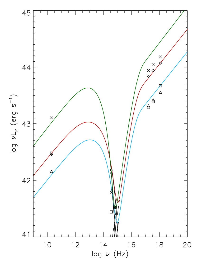
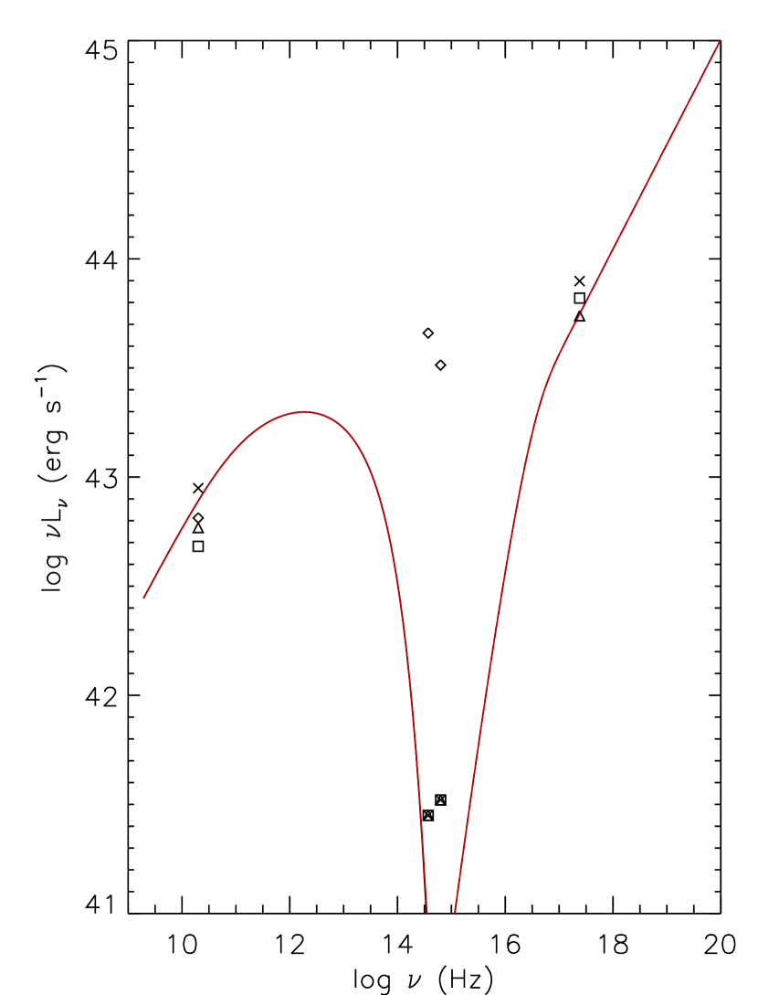
Figure 11.— Spectral energy distributions (SEDs) for the core plus four regions of the jet of 0208–512 (left) and 1202–262 (right). For the jet of 0208–512, data points for K0 are shown as diamonds, those for K1 are triangles, those for K2 are squares, and the data for K3 are X’s. For the jet of 1202–262, data points for R0 are diamonds, data for R1 are triangles, those for R2 are squares, and the data for R3 are X’s. With the exception of R0 in the 1202–262 jet, all the F475W points are upper limits, as is the case for the F814W points for 0208–512 K2, 1202–262 R1, 1202–262 R2 and 1202–262 R3. The most likely interpretation for the optical emission of the detected knots of both jets is the extreme tail of synchrotron emission, while the X-ray emission is most likely due to inverse-Comptonization of CMB photons (IC-CMB), as discussed in §4.2. We have overplotted Synchrotron/IC-CMB models of jet components, as detailed in §4.2.2. For 0208–512, we show models for regions K0 (red), K1 (blue) and K3 (green); a model is not shown for K2 since it is essentially identical to that for K2. For 1202, we show only the model for R1, as the models for R2 and R3 are essentially identical. No model is fitted for R0 in the 1202 -262 jet as the knot is not fully resolved in X-rays, making it difficult to constrain the IC-CMB component.

We now apply the method laid out in §4.3 to calculate physical parameters for the jets of 0208–512 and 1202–262, under the assumption that the X-ray emission from them arises via the EC/CMB scenario. We adopt a single spectral index $\alpha=(p-1)/2$, equal to that observed in the radio (i.e., 0.69 for 0208–512 and 0.52 for 1202–262). These spectral indices are consistent with those observed in the X-rays, as would be expected under the EC/CMB model. We adopt a uniform magnetic field and assume the equipartition condition. We also assume that the emitting volume is a cylinder, with a filling factor of unity and assume that the ratio of proton to electron energy density is also 1. All emitting volumes are taken to be cylinders with the measured angular lengths, and radii of 0.5 arcseconds. We assume a moving blob for each feature with the given values of $\delta$, $B$, etc. (as opposed to a standing shock). The minimum particle energy was chosen as $\gamma_{min}=15$. These assumptions result in the values laid out in Table 3. The resulting spectral energy distributions are plotted in Figure 11. The typical error ranges on these parameters are $\sim 10\%$, so that, for example, the jet of PKS 1202–262 is consistent with a constant $\delta$ and $\theta$ for all components. Note too that in estimating these parameters we assumed that the same volume is radiating for both the radio and X-ray, whereas in Figure 9 and accompanying text we have noted differences between the X-ray and radio morphologies for both jets. To calculate the jet kinetic power, one needs to select a viewing angle. For PKS 0208–512, we have chosen a value of $\theta=3^{\circ}$ , which was the mean angle to the line of sight for the MOJAVE sample (Hovatta et al. 2009), whereas for PKS 1202–262, which is required to be more highly beamed ($\delta>20$ and $\theta<2.5^{\circ}$) we chose $\theta=2^{\circ}$. The jet powers reported in Table 3, would increase by a factor of $m_{p}(p-2)/[m_{e}(p-1)\gamma_{min}]$ if we assume instead that for every radiating electron there is a cold proton. The result would be an increase in jet power by a factor of $\approx 34$ for 0208–512 and $\approx 2$ for 1202–262. Even with this increase – which corresponds to the limiting case, under rough equipartition conditions, of the absence of positrons – the jet powers remain smaller or at most comparable to the Eddington luminosity of a $10^{9}M_{\odot}$ black hole.

Table 3Properties of the X-Ray Jet Components

Object	Region	$B~{}(\mu$G)	$\delta$	$\theta_{\rm max}$ (deg)	$L_{com}^{\rm a}$	$P_{jet}^{\rm b}$
0208–512	K0	8.7	10.2	5.6	1.03	2.10
	K1	8.8	8.3	6.9	1.06	1.36
	K2	12.0	7.5	7.7	1.96	2.00
	K3	13.9	9.5	6.0	2.65	4.60
1202–262	R1	4.9	22.5	2.5	0.31	3.84
	R2	4.2	24.8	2.3	0.23	3.99
	R3	5.3	23.4	2.4	0.36	1.42

5. Discussion

We have analyzed deep Chandra and HST observations of the jets of PKS 0208–512 and PKS 1202–262. Both jets can be seen in the X-ray images extending for several arcseconds from the quasar, and both exhibit at least one optically detected component. The observed X-ray characteristics of both jets are consistent with the popular IC-CMB model but are difficult to explain under models where the X-ray emission is due to the synchrotron process. In this context, we have presented a method to analyze the X-ray emission of jets and solve independently for the beaming factor $\delta$ and magnetic field $B$.

The two jets appear to illustrate two rather different ranges of parameter space. It is apparent that the jet of PKS 0208–512 requires higher magnetic fields and lower beaming parameters $\delta$, and a greater angle to the line of sight than the jet of PKS 1202–262. We find only weak evolution, if any, of the physical parameters with distance from the nucleus in both jets (Table 3). In 0208–512 there is evidence for a consistent increase in magnetic field with increasing distance from the nucleus; however, a similar pattern is not seen in 1202–262. While there is some change in the Doppler factor the jet of PKS 0208–512, it is not systematic in either one. Changes in the Doppler factor would produce differences between the observed radio and X-ray morphology (Georganopoulos & Kazanas 2004), in the sense that in a gradually decelerating jet we would expect X-ray knots to lead those seen in the radio, due to additional emission from the upstream Compton mechanism. However, looking at Figure 9, it is interesting to note that there are significant radio/X-ray morphology differences in both jets. As can be seen, the X-ray fluxes of several jet components do appear to be located closer to the nucleus than the corresponding radio maxima. This is in line with the predictions of the upstream Compton scenario of Georganopoulos & Kazanas (2004) but does not require changes in the jet speed or trajectory with increasing distance along the jet.

References

- (1) Arshakian, T. G., & Longair, M. S. 2004, MNRAS, 351, 727
- (2) Atoyan, A. M., & Dermer, C. D., 2004, ApJ, 613, 151
- (3) Bertsch, D. L., et al., 1993, ApJ, 405, L21
- (4) Blom, J. J., et al., 1995, A&A, 298, L33
- (5) Blom, J. J., et al., 1996, A&A Supp., 120, 507
- (6) Bolton, J. G., Gardener, F. F., Mackey, M. B., 1964, Aust. J. Phys, 17, 340
- (7) Celotti, A., Ghisellini, G., & Chiaberge, M., 2001, MNRAS, 321, L1
- (8) Chartas, G., et al., 2000, ApJ, 542, 655
- (9) Dermer, C. D., 1995, ApJ, 446, L63
- (10) Dermer, C. D., & Atoyan, A. M., 2002, ApJ, 568, L81
- (11) Dermer, C. D., & Atoyan, A. 2004, ApJ, 611, L9
- (12) Deutsch, E. W., 1999, AJ, 118, 1882
- (13) Felten, J. E., & Morrison, P. 1966, ApJ, 146, 686
- (14) Gelbord, J. M., et al., 2005, ApJ, 632, L5
- (15) Georganopoulos, M. & Kazanas, D., 2004, ApJ, 604, L81
- (16) Georganopoulos, M., Kazanas, D., Perlman, E. S., Stecker, F. W., 2005, ApJ, 625, 656
- (17) Georganopoulos, M., Kazanas, D., Perlman, E. S., McEnery, J., 2006, ApJ, 653, L5
- (18) Georganopoulos, M., Kazanas, D., Perlman, E. S., Wingert, B., 2010, in prep.
- (19) Georganopoulos, M. Kirk, J. G., & Mastichiadis, A. 2001, ApJ561, 111
- (20) Godfrey, L. E. H., et al., 2009, ApJ, 695, 707
- (21) Ghisellini, G., & Celotti, A., 2001, MNRAS, 327, 793.
- (22) Hardcastle, M. J., 2006, MNRAS, 366, 1465
- (23) Harris, D. E., Krawczynski, H., 2006, ARAA, 44, 463
- (24) Jester, S., Harris, D. E., Marshall, H. L., Meisenheimer, K., 2006, ApJ, 648, 900
- (25) Jester, S., Meisenheimer, K., Martel, A. R., Perlman, E. S., Sparks, W. B., 2007, MNRAS, 380,828
- (26) Jester, S., Röser, H.–J., Meisenheimer, K., Perley, R., Conway, R., 2001, A&A, 373, 447
- (27) Jorstad, S., & Marscher, A., 2004, ApJ, 614, 615
- (28) Kirk, J. G., Guthmann, A. W., Gallant, Y. A., Achterberg, A., 2000, ApJ, 542, 235
- (29) Koekemoer, A. M., Fruchter, A. S., Hook, R., Hack, W., 2002 HST Calibration Workshop (PASP), p. 337. See also http://www.stsci.edu/hst/acs/analysis/multidrizzle.
- (30) Krist, J. E., & Burrows, C. J., 1994, WFPC2 ISR 94-01
- (31) Krist, J. E., & Hook, R., 2004, ”The TinyTim User’s Guide, Version 6.3”,
- (32) http://www.stsci.edu/software/tinytim/tinytim.pdf
- (33) Lovell, J. E. J. et al., 2000, in Astrophysical Phenomena Revealed by Space VLBI, Eds. H. Hirabayashi, P. G. Edwards & D. W. Murphy (Sagamihara: ISAS), 215
- (34) Marshall, H. L., et al., 2005, ApJS, 156, 13 (Paper I)
- (35) Marshall, H.. L., et al., 2011, ApJS, 193, 15
- (36) Mehta, K. T., Georganopoulos, M., Perlman, E. S., Padgett, C. A., Chartas, G., 2008, ApJ, submitted
- (37) Ostrowski, M., 2008, New Astron. Rev. in press, also astro-ph/0801.1339
- (38) Perlman, E. S., Wilson, A. S., 2005, ApJ, 627, 140
- (39) Peterson, B. A., Wright, A. E., Jauncey, D. L., Condon, J. J., 1979, ApJ, 232, 400
- (40) Rawlings, S., Saunders, R., 1991, Nature, 349, 138
- (41) Sambruna, R. M., 1997, ApJ, 487, 536
- (42) Sault, R. J., Teuben, P. J., Wright, M. C. H., 1995, in Proc. ADASS IV Meeting, ed. R. A. Shaw, H. E. Payne & J. E. Hayes, ASP Conference Series, 77, 433
- (43) Schwartz, D. A., et al., 2000, ApJ, 540, L69
- (44) Schwartz, D. A., et al, 2006a, ApJ, 640, 592 (Paper II)
- (45) Schwartz, D. A., et al., 2006b, ApJ, 647, L101
- (46) Schwartz, D. A., et al., 2007, Ap & SS, 311, 341
- (47) Shen, Z.-Q., Wan, T.-S.; Hong, X.-Y., Jiang, D.-R.; Liang, S.-G., 1998, Ch A&A, 22, 1
- (48) Shepherd, M. C., 1997, in Proc. ADASS VI Meeting, ed. G. Hunt & H. Payne, ASP Conference Series, 125, 77
- (49) Spergel, D. N., et al., 2003, ApJS, 148, 175
- (50) Stacy, J. G., Vestrand, W. T., Sreekumar, P., Bonnell, J., Kubo, H., Hartman, R. C., 1996, A&A Supp., 120, 549
- (51) Suchkov, A., & Krist, J., 1998, NICMOS ISR 98-018
- (52) Tavecchio et al., 2002, ApJ, 575, 137
- (53) Tavecchio, F., Maraschi, L., Sambruna, R. M., Urry, C. M., 2000, ApJ,544, L23
- (54) Tavecchio, F., Maraschi, L., Wolter, A., Cheung, C. C., Sambruna, R. M., Urry, C. M., 2007, ApJ, 662, 900
- (55) Tingay et al., 1996, ApJ, 464, 170
- (56) Tingay et al., 2002, ApJS, 141, 311
- (57) Uchiyama, Y., Urry, C. M., van Duyne, J., Cheung, C. C., Sambruna, R. M., Takahashi, T., Tavecchio, F., Maraschi, L., 2005, ApJ, 631, L113
- (58) Uchiyama, Y., Urry, C. M., Cheung, C. C., Jester, Sebastian, Van Duyne, J., Copppi, P., Sambruna, R. M., Takahashi, T., Tavecchio, F., Maraschi, L., 2006, ApJ, 648, 910
- (59) Wills, B. J., Wills, D., Douglas, J. N., 1973, AJ, 78, 521
- (60) Worrall, D. M., 2009, A&A R, 17, 1
- (61) Worrall, D. M. & Birkinshaw, M. 2006, in ’Physics of Active Galactic Nuclei at all Scales’, edited by Danielle Alloin, Rachel Johnson and Paulina Lira Lecture Notes in Physics, 693, 39
- (62) Worrall, D. M., Birkinshaw, M., Hardcastle, M. J., 2001, MNRAS, 326, L7
- (63)