Horizon synthesis for archaeo-astronomical purposes

Abstract

In this paper I describe a simple numerical procedure to compute synthetic horizon altitude profiles for any given site. The method makes use of a simplified model of local Earth’s curvature, and it is based on the availability of digital elevation models describing the topography of the area surrounding the site under study. Examples constructed using the Shuttle Radar Topographic Mission (SRTM) data (with 90m horizontal resolution) are illustrated, and compared to direct theodolite measurements. The proposed method appears to be reliable and applicable in all cases when the distance to the local horizon is larger than $\sim$10 km, yielding a rms accuracy of $\sim$0.1 degrees (both in azimuth and elevation). Higher accuracies can be achieved with higher resolution digital elevation models, like those produced by many modern national geodetic surveys.

1 Introduction

When studying the orientation of buildings, tombs, or any other man made structure, having an handy description of the natural horizon is a fundamental step. In most of the cases this is done directly measuring the horizon altitude at the relevant azimuths using, for instance, a theodolite and sun fixes. Depending on the angular sampling one wants to achieve, this might turn into a rather long and boring procedure. An alternative possibility is the calibration of a few points using direct theodolite readings coupled to digital, rectified photography. However, this might turn to be difficult, or even impossible, in the case the natural horizon is not visible because of modern constructions or vegetation.

In this paper I propose an alternative solution, which is based on a simple geometrical model for Earth’s local shape and the availability of a digital elevation model (DEM) for the area under examination. The idea is rather simple. For a given observer’s site, the line of site (hereafter LOS) elevation profile (LOSEP) along the input azimuth is extracted. Then, for each point along the LOS, the apparent altitude above the local horizontal is estimated and the maximum is found. By definition, this is the natural horizon altitude as seen from the observing site. Repeating the same procedure for all azimuths (with a given angular step) will finally allow one to retrieve the horizon altitude profile. The angular resolution clearly depends on the horizontal sampling in the DEM, while the accuracy is related to the DEM vertical accuracy.

Since the available DEMs provide the elevation above a given ellipsoid (typically the WGS84), the first thing one needs to take into account is Earth’s curvature, which makes a far mountain appear lower than it would if the Earth’s surface were flat. Then, although this is a second order effect, one has to correct for the terrestrial refraction (which has the opposite effect). These two corrections are discussed in the next two sections.

2 Correcting for Earth’s curvature

Let us consider an observer placed in $A$ at an elevation $h_{A}$ (above the sea level), and a point $B$ (elevation $h_{B}$), located at a distance $d$ from A. If Earth were flat, the altitude $\alpha$ of $B$ seen from $A$ would simply be:

$$\alpha=\arctan\left(\frac{h_{B}-h_{A}}{d}\right).$$

However, because of Earth’s curvature, far objects subtend altitudes which are smaller than those given by the previous expression. Using a simplified model for Earth’s local curvature, one can derive the following approximate expression (see Appendix A):

$$\alpha\approx\arctan\left[\frac{h_{B}-h_{A}}{d}-\frac{1}{2}\frac{d}{R}\right],$$ (1)

where $R$ is the local radius of curvature (see Equation 4). For example, suppose that a $h_{B}$=3.0 km mountain peak is observed from a site placed $d$=100 km away, at an elevation $h_{A}$=0.1 km. Using $R$=6370 km one obtains $\alpha$=1^∘.21. Neglecting Earth’s curvature one would get $\alpha$=1^∘.66, almost half a degree off. It can be easily shown that for ellipsoidal distances $d\leq$300 km the error introduced by the approximated expression (1) is less than 0.01 degrees, which is well below the typical archaeoastronomical needs.

In the cases where $|h_{B}-h_{A}|/d\ll 1$, using Equation 1 one can show that the apparent altitude decreases at a rate of $1/2R$, which is about 16^′′.2 km^-1 (or 0^∘.0045 km^-1).

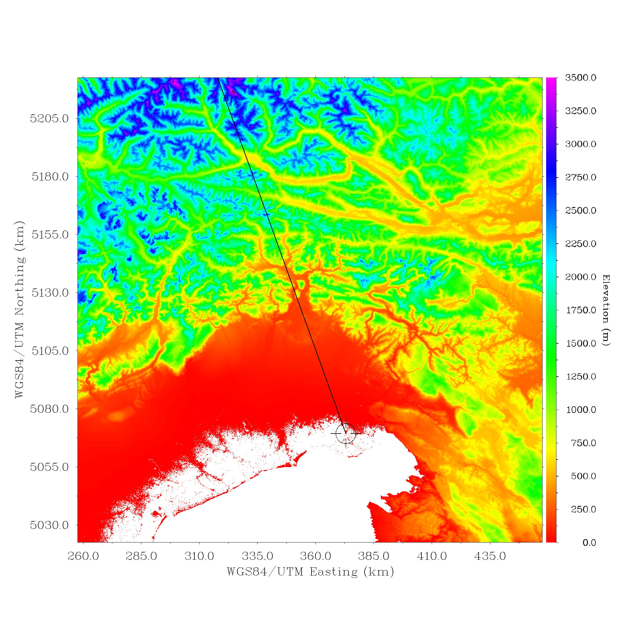
Figure 1: Example LOSEP extraction for the Roman town Aquileia ($\lambda$=13^∘.367 E, $\phi$= 45^∘.767 N), with $\varphi$=339^∘. The underlying DEM is from the SRTM90 data set, and is displayed in the Universal Transverse Mercator projection (UTM, 33N). The white area in the lower part of the map is the Adriatic Sea.

3 Correcting for terrestrial refraction

As the light travels across Earth’s atmosphere it bends, in such a way that a far object appears to be higher than actually is. This phenomenon is known as terrestrial refraction.

If $\alpha$ is the unrefracted horizon altitude (corrected for Earth’s curvature), then the apparent horizon altitude $\alpha^{\prime}$ is simply given by $\alpha^{\prime}=\alpha+R_{T}$. Several analytical descriptions of $R_{T}$ have been proposed, but the one developed by Bomsford ([1980]) appears to be the most accurate (see for instance Sampson et al. [2003]). In this formulation the terrestrial refraction is given by

$$R_{T}=\kappa d\;,$$

where $d$ is the distance between the observer an the natural horizon (in km), and $\kappa$ (degrees km^-1) is defined as:

$$\kappa=\frac{1}{R}\frac{0.252P}{T^{2}}\left(34.2+\frac{dT}{dz}\right)\frac{180}{\pi}\;,$$ (2)

where $R$ is Earth’s radius (in km), $P$ is the atmospheric pressure (in millibars), $T$ is the ground air temperature (in K), and $dT/dz$ is the ground atmospheric vertical temperature gradient (in K km^-1). For typical atmospheric conditions ($P$=1000 mb, $T$=293 K, $dT/dz$=$-$10 K km^-1) one finds that $\kappa\sim$2.3 arcsec km^-1 (or 0.00064 degrees km^-1). This is about seven times smaller than the effect produced by Earth’s curvature. In the case of the example discussed in the previous section ($d$=100 km) this would turn into a correction of $\sim$0.06 degrees.

One can simplify the previous formula introducing the refraction constant $K$:

$$K=0.273\left(34.2+\frac{dT}{dz}\right)\;.$$

With this setting, $\kappa$ (in degrees km^-1) can be written as:

$$\kappa=0.00829\;K\;\frac{P}{T^{2}}\;.$$ (3)

Typical values of $K$ range from $\sim$5 (during the day) to $\sim$10 (at sunset/sunrise or night). The fluctuation of atmospheric conditions introduce a variation in $\kappa$, which can range from $\sim$1.5 to $\sim$4 arcsec km^-1. For instance, on a distance of 100 km this translates into a peak-to-peak horizon altitude change of $\sim$0.07 degrees. Therefore, even in the hypothesis all other quantities are known with negligible errors, this sets the natural maximum accuracy one can achieve on the horizon apparent altitude.

4 Digital Elevation Model

The proposed method is based on the availability of a DEM, i.e. an array of values giving the elevation of a given point above the underlying ellipsoid. If $\lambda$ and $\phi$ are the longitude and latitude of a point $\vec{P}$ on the ellipsoid, I will express its elevation $z$ as $z=g(\lambda,\phi)$ or, alternatively, as $z=g(\vec{P})$.

Because of its nature, a DEM is a discrete collection of data points, obtained with some spatial resolution. Typically, the data are distributed on a regular grid, with a horizontal sampling that I will indicate as $\Delta l$. This corresponds to the minimum scale one can resolve in the DEM. Obviously, if one is to get the elevation of a point which does not coincide with one of the grid nodes, then one will have to use some interpolation method (nearest neighbor, linear interpolation, bi-cubic spline interpolations, etc). No matter what method is used, though, the resolution is dictated by the sampling. In the following I will assume that the DEM is given with a regular sampling $\Delta l$, which is to say that the data points have been obtained/re-gridded at a constant step. Also, I will indicate with $\sigma_{z}$ the rms uncertainty on each DEM data point.

Each country has its own geographical survey program-me, aiming at mapping its territory with a certain resolution. These data may or may not be available to the reader. Therefore, in this article I will consider the Shuttle Radar Topographic Mission, which has the advantage of having a relatively good horizontal resolution, a good vertical accuracy, an almost world wide coverage, and, most importantly, is freely available.

4.1 The Shuttle Radar Topographic Mission

The Shuttle Radar Topographic Mission (SRTM) provides an homogeneous coverage of Earth’s elevation (Farr et al. [2007]). For the US territory it is distributed with a horizontal resolution of 30 m (SRTM30), while for the rest of the planet data were averaged within bins of 90$\times$90 m² (SRTM90), hence including 3$\times$3 original data points each. The 90%-level absolute vertical accuracy of the SRTM original data is better than 9 m (Farr et al. [2007]), which corresponds to an rms accuracy of 5.5 m. Therefore, the formal rms error on the 90 m data is expected to be $\sigma_{z}\sim$1.8 m. I note, however, that this is strictly true only if the terrain is smooth on scales smaller than 30 m, otherwise the averaging process within 90 m bins produces an artificial smoothing, turning into much larger deviations from the real values. Clearly this is going to affect very steep mountain regions, where the elevation can change significantly on scales of tens of meters. As a consequence, sharp mountain peaks appear in the SRTM90 data with lower than real elevations.

The altitude uncertainty $\sigma_{\alpha}$ (in degrees) implied by an elevation uncertainty $\sigma_{z}$ can be estimated through the following approximate expression:

$$\sigma_{\alpha}\approx\frac{180\sqrt{2}}{\pi}\;\frac{\sigma_{z}}{d}\;,$$

where $d$ is the distance between the observer and the point being surveyed, expressed in the same units as $\sigma_{z}$. For instance, the formal elevation error of the SRTM90 data (1.8 m) translates into an altitude error of about 0.1 degrees at $d\simeq$1.5 km.

As for the SRTM horizontal accuracy, this is better than 20 m (at the 90%-level; Farr et al. [2007]). This corresponds to an rms deviation $\sigma_{l}$=14 m). Therefore, in the SRTM90 case, this is much better than the horizontal resolution $\Delta l$. As a consequence, the rms error on the azimuth $\varphi$ of a given data point is approximately

$$\sigma_{\varphi}\approx\frac{180}{\pi}\;\frac{\sigma_{l}}{d}\simeq\frac{0.8}{d_{km}}\;.$$

At $d$=10 km this corresponds to an uncertainty of $\sim$0.1 degrees, which is a fifth of the apparent diameter of the sun (and the moon). Obviously, if the horizon is farther away, the azimuth uncertainty becomes proportionally smaller. If one is after higher azimuth accuracies, or the horizon in the direction of interest is closer than 10 km, then a DEM with better sampling is required.

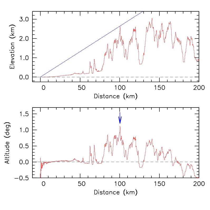
Figure 2: Upper panel: LOSEP along $\varphi$=339^∘ for the Roman town of Aquileia (see Figure 1). Lower panel: the corresponding altitude profile. The blue arrow marks the maximum altitude, corresponding to the natural horizon along the chosen direction.

In this respect, I note that a preliminary version of the data produced by the Advanced Spaceborne Thermal Emission and Reflection Radiometer (ASTER) was recently released. Nominally they have an horizontal resolution of 30 m, which is a factor 3 better than the SRTM90. However, a close look to the data shows that the effective horizontal resolution is actually close to 90 m and the vertical accuracy is not as good as the one of SRTM, at least not in the released version.

5 LOSEP extraction and horizon determination

Having a DEM at hand, one can extract the LOSEP starting from the observer’s position $\vec{P_{0}}$ along a given azimuth $\varphi$ as a function of distance $d$ from the observer. This corresponds to solving the forward geodesic problem, i.e. computing the running end point $\vec{P}$ of a geodesic path on the ellipsoid, given the start point $\vec{P_{0}}$, a path length $d$, and a starting azimuth $\varphi$. As is standard in geodesy, this is done numerically, using the iterative algorithm devised by Vincenty ([1975]). Although the solution is non-analytical, for the sake of clarity I will indicate it as

$$\vec{P}=f(\vec{P_{0}},d,\varphi)\;.$$

Given the discrete nature of the DEM, the LOSEP is extracted at a number of points, which are separated by some constant length. Obviously, the maximum resolution is attained when this length is equal to the DEM resolution $\Delta l$.

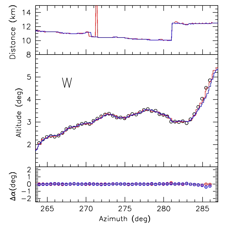
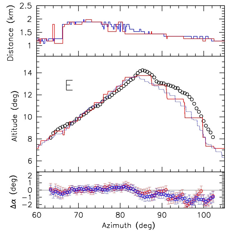
Figure 3: Comparison between the theodolite readings (empty circles) and the synthetic profiles (W to the left and E to the right) computed using SRTM (red) and ASTER (blue) DEMs for the site of St. Martin (Artegna - Italy). Top panel: horizon distance. Middle panel: horizon profiles. Bottom panel: $\Delta\alpha$ residuals (computed$-$measured). The errorbars indicate the 5-$\sigma$ error of the synthetic profile.

With these definitions, the LOSEP extraction is done through the following steps:

1. elevation $z_{0}=g(\vec{P_{0}})$ is extracted from the DEM at ($\lambda_{0},\phi_{0}$);

2. the path length for the $i$-th step along the LOS is updated to $d_{i}=\Delta l\;i$;

3. the coordinates ($\lambda_{i},\phi_{i}$) of the running point $\vec{P}$ are computed as $f(\vec{P_{0}},d_{i},\varphi)$

4. the elevation of the running point is computed as $z_{i}=g(\lambda_{i},\phi_{i})$;

5. the apparent altitude $\alpha_{i}$ of $\vec{P}$ as seen from $\vec{P_{0}}$ is calculated with Equation 7 and corrected for terrestrial refraction;

6. the cycle is repeated from step 2, until $d_{i}$ reaches a maximum value $d_{max}$.

Once this is done, the horizon elevation along azimuth $\varphi$ is determined as $\alpha(\varphi)=\mbox{max}\{\alpha_{i}\}$. I note that in most of the cases it is sufficient to consider distances within $d_{max}\simeq$200 km. The exact value depends on the maximum elevation in the area surrounding the site under study. From Equation 1, one has that the distance at which a mountain peak appears at an altitude $\alpha$=0 is given by $d\approx\sqrt{2R\Delta z}$, where $\Delta z$ is the difference in elevation. For $\Delta z\leq$4.0 km (which is true for most of the sites on the planet), it is $d\leq$225 km. Incidentally, here emerges one of the advantages of horizon synthesis over direct measurements. If the horizon is far away ($d>$50-100 km), it might be very difficult, if not impossible, to have a sufficient atmospheric transparency to be able to actually see it.

An example LOSEP extraction is presented in Figure 1, where I have chosen the Roman town Aquileia (Italy; founded in 181 BCE) as the observing site. For the sake of the example I have traced the LOS along one of the two cardinal directions of the town ($\varphi\simeq$339^∘), in the NW direction. The site is marked with a circle, while the selected line of sight is traced by a solid line. The underlying DEM (from the SRTM90 data set) has been projected to the Universal Transverse Mercator system (see Hager, Behensky & Drew [1989]).

The LOSEP extracted along this direction is shown in Figure 2 (upper panel), and it reaches about 3000 m in the Austrian Alps, at a distance of 140 km from Aquileia. However, the horizon is located at about 100 km, at an elevation of $\sim$2600 m, and it subtends an apparent altitude of $\sim$1^∘.1 (Figure 2, lower panel).

Clearly the whole process can be repeated for $\varphi$ ranging from 0^∘ to 360^∘ with a given step $\Delta\varphi$. This will finally give the full horizon profile $\alpha(\varphi)$.

6 Validation

The simplest way of validating the procedure outlined in the previous section is a comparison between the synthetic profile and direct horizon measurements. The natural horizon altitude can be determined using a theodolite and sun fixes, taking measurements with some azimuth step. The typical accuracy one can achieve with this method is of the order of a tenth of a degree or better, depending on the quality of the instrument used.

In the course of studying the orientation of the ancient church of St. Martin (Artegna - Italy; 13^∘.1528 E, 46^∘.2415 N, 267 m a.s.l.), I had measured the natural horizon altitude in a range around E and W directions. The building is located on top of St. Martin Hill, about 50 m above the surrounding plain. The E horizon is dominated by the presence of Mt. Faet (750 m a.s.l.), whose top is located at less than 2 km from St. Martin. Seen from the site, the top subtends an angle of about 14 degrees. On the contrary, the W§ horizon is located at more than 10 km, and has an altitude around 3 degrees. The different distances to the E and W horizon locations from the observing site make this an ideal test case. The comparison between the theodolite readings and the synthetic profile is presented in Fig. 3.

In the case of the W horizon, the deviations are always smaller than 0.2 degrees, and in most of the cases they are less than 0.1 degrees, i.e. well within the expected rms errors. In general, the SRTM DEM gives a better result than the ASTER one (Fig. 3, left panels). Things are different for the E horizon, for which the match is good only along the smooth declining ridge of Mt. Faet in the azimuth range 68^∘–78^∘, where the horizon is at a distance of about 1.9 km (Fig. 3, right panels). Between 64^∘ and 68^∘, where the distance drops to about 1.2 km, the deviations exceed 0^∘.5. But the largest discrepancies are seen for azimuths larger than 84^∘, where they are larger than 1^∘.5. This very clearly illustrates the effect of a close horizon coupled to a steep slope, where the smoothing intrinsic to the DEM data produces systematically lower elevations and, in turn, altitudes.

These two examples demonstrate that the procedure described here, when used in conjunction to SRTM90 or ASTER DEMs, gives results accurate to $\sim$0.1 degrees only for horizon distances larger than $\sim$10 km. This does not exclude that acceptable results may be achieved also for shorter distances, but this will depend on the horizon morphology, and cannot be assumed a priori.

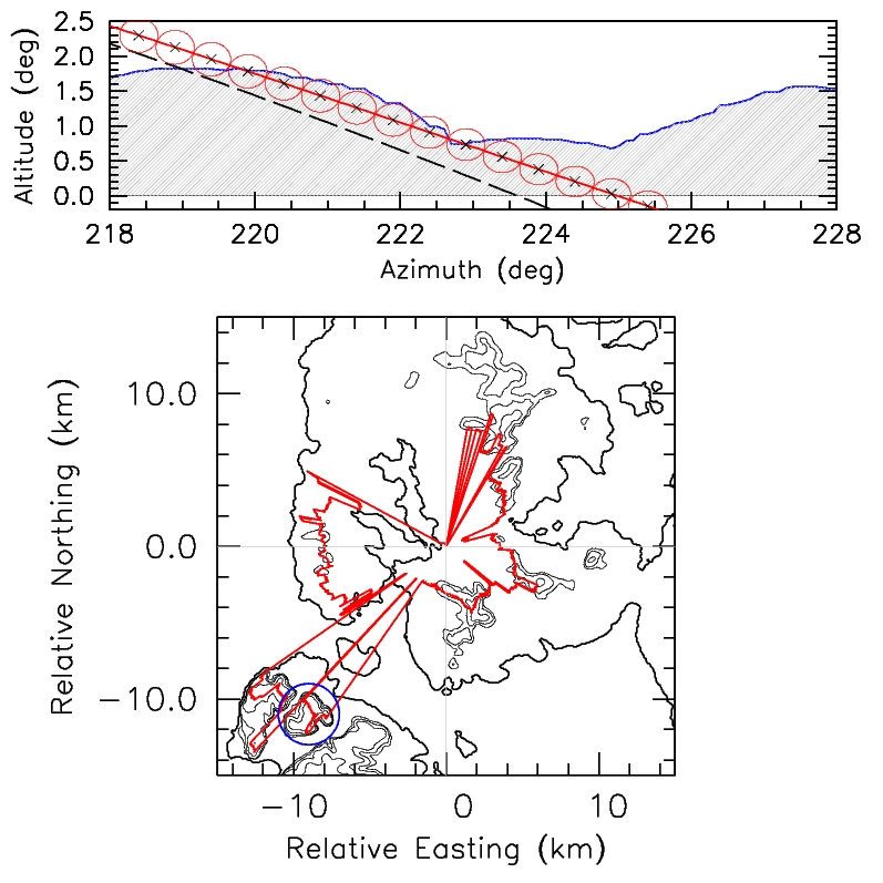
Figure 4: Lower panel: horizon location for Maes Howe. The map is a contour plot of the SRTM DEM. The position of Ward Hill is marked by a blue circle. Upper panel: apparent path of the sun on December 1st ($\delta_{\odot}$=$-$21^∘.9; solid red line). The dashed line traces the real path of the sun (see text). The red circles mark the position of the sun (to scale) with a time interval of 2 minutes. The blue curve is the SRTM synthetic horizon as seen from Maes Howe.

7 Example application: the case of Maes Howe

The method described in this paper can be applied any time there is the need of having a handy description of the natural horizon in an archaeo-astronomical analysis. To show the potential of the technique, I close this article with an application to a famous and well studied case, where the horizon shape is playing a fundamental role: Maes Howe.

Maes Howe is a neolithic site located on Mainland, Orkney, Scotland (3^∘.1879 W, 58^∘.9981 N, 20 m a.s.l.). Besides being the site of a chambered cairn and passage grave, Maes Howe offers a spectacular event. Around twenty days before (and after) the winter solstice, the sun sets below the horizon defined by Ward Hill, placed at about 14 km SW of Maes Howe. However, after 7-8 minutes, it reappears for a couple of minutes, just before definitely setting (Reijs [1998, 2001]. See also Magli [2009], his Figs. 3 and 4). This is due to a combination of the sun apparent path and the morphology of the horizon.

This phenomenon is very well reproduced using the synthetic horizon computed for Maes Howe, once one applies a standard astronomical refraction correction to the position of the sun. This is illustrated in Fig. 4, where I have traced the apparent trajectory of the sun over the horizon. The sun reappears for a couple of minutes at an azimuth around 223^∘, in full agreement with direct measurements (Reijs [1998]), when the sun declination is $\delta_{\odot}$=$-$21^∘.9 (corresponding to December 1st of today’s calendar). An accurate reproduction is obtained also for the sun reappearance in the direction of Kame of Hoy, which takes place for $\delta_{\odot}=-$17^∘.3 (February 1st), at an azimuth of about 235^∘.5. Since in 2700 BCE (the supposed date for the construction of Maes Howe) the obliquity was about 23^∘.8, things were not very much different, and the same phenomenon took place about 22 days before and after winter solstice. Having the synthetic horizon, one can now ask what would be the azimuth of the setting sun on the solstice. This turns out to be 216^∘.8 (disk center), and the horizon altitude is 1^∘.3, but in this case no reappearance is possible. As minimum and maximum azimuths for which the sun can shine on the back of the chamber are approximately 217^∘ and 223^∘ (Reijs [1998]), both the solstice setting and the sun reappearance should be observable from within the chamber itself.

The procedure outlined in this paper could be used, for instance, to test whether the reappearing sun is visible from other sites of archaeological relevance close to Maes Howe. As an example I analyze the case of the Ring of Brodgar (3^∘.2280 W, 59^∘.0014 N). This stone circle, located between the Lochs of Stenness and Harray, has a diameter of about 104 m, and is the third largest in the British Isles (Ruggles [1999]). As the calculations show, around $\pm$20 days from winter solstice the sun sets over the Kame of Hoy, about 10^∘ S of Ward Hill, without re-emerging from behind it (Fig. 5, top panel). At present day’s winter solstice, the sun still sets behind the Kame of Hoy, without re-appearing (Fig. 5, middle panel). Even for the increased obliquity expected for 2700 BCE the apparent sun path does intersect the profile of Ward Hill. On the contrary, the reappearance of the sun is in principle observable from the Ring of Brodgar when $\delta_{\odot}$=$-$20^∘.1 (November 22/January 21), that is about one month before and after winter solstice (Fig. 5, bottom panel).

8 Conclusions

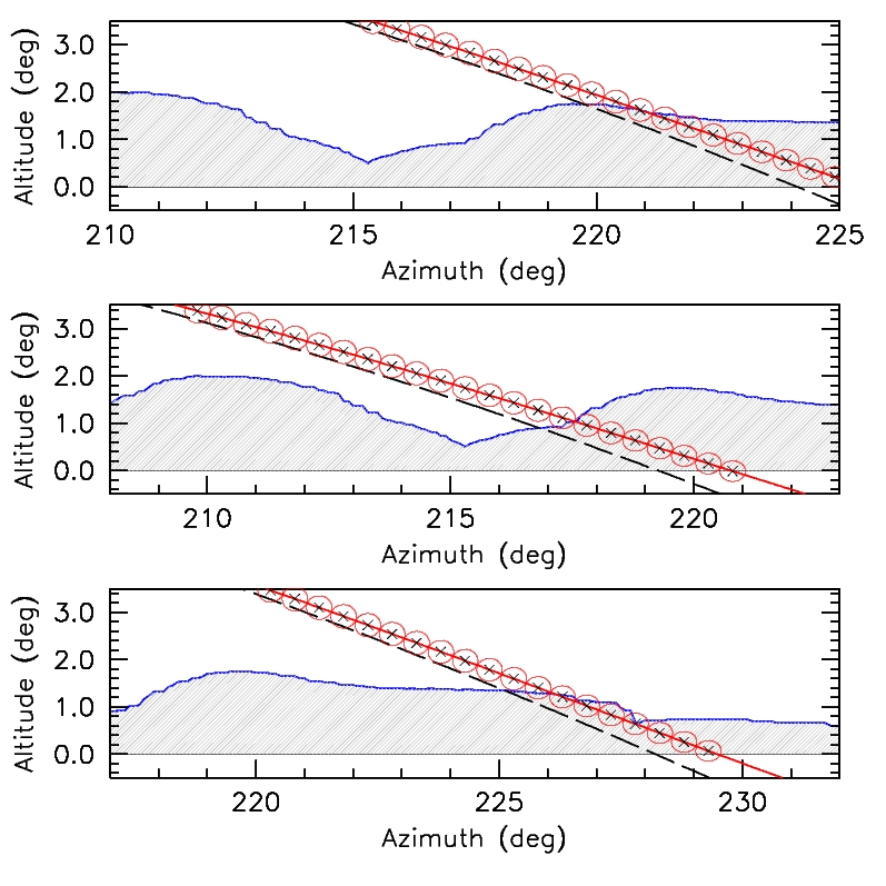
Figure 5: Synthetic horizon computed for the Ring of Brodgar and apparent sun path for $\delta_{\odot}$=$-$21^∘.7 (top), $-$23^∘.5 (middle), and $-$20^∘.1 (bottom).

The procedure I have outlined in this paper allows one to easily compute a synthetic horizon profile for any site. The accuracy in the final product depends on the resolution of the DEM and its vertical accuracy. Rms deviations of $\sim$0^∘.1 degrees are achievable with the SRTM90 data when the horizon is at distances of the order of 10 km. For shorter distances, the deviations are expected to be larger, especially if the horizon is defined by steep mountain profiles. In those cases the morphology of the area surrounding the site of interest needs to be examined more closely, and the synthetic horizon validated with direct theodolite measurements obtained along some critical directions.

The method can be applied during the exploratory phase of an archaeoastronomical site’s study, either to plan direct on-site surveys or to test working hypotheses. When accuracies of a few tenths of a degree are sufficient (as is certainly the case for solar alignments), the results provided by the method can be used directly for the orientation analysis, saving a significant amount of time during the field work.

Appendix A Derivation of Earth’s curvature correction

In the following I will assume Earth can be described by an ellipsoid with semi-axis $a$ and $b$. However, for the sake of simplicity, I will also assume that locally it can be approximated by a sphere having the curvature radius of the ellipsoid at the site under examination. If $\phi$ is the site geodetic latitude, this is given by

$$R(\phi)=\frac{ab}{\sqrt{a^{2}\sin^{2}\phi+b^{2}\cos^{2}\phi}}\;.$$ (4)

Throughout this paper I adopt the WGS84 ellipsoid, which has $a$=6378.1 km and flattening $f$=1.0/298.25722356 ($b$=6356.8 km). If we now imagine to have an observer placed in $A$, at elevation $h_{A}$ above the ellipsoid, looking at a site $B$ placed at elevation $h_{B}$ and with an angular separation on the ellipsoid defined as $\theta$ (see Figure 6), the altitude $\alpha$ of $B$ as seen from $A$ above the local horizontal plane is given by

$$\alpha=\arctan\left(\frac{h^{\prime\prime}}{d^{\prime\prime}}\right)\;,$$ (5)

where $d^{\prime\prime}$ and $h^{\prime\prime}$ are defined as in Figure 6. While $d^{\prime\prime}$ is the distance between $A$ and $B$ projected on the local horizontal plane, $h^{\prime\prime}$ is the elevation of $B$ above the same plane. The whole problem reduces to determining these two lengths.

Looking at Figure 6 we immediately note that:

$$d^{\prime\prime}=\left(R+h_{B}\right)\;\sin\theta\;.$$

If we define $\Delta h=HH^{\prime}$ (see Figure 6), then we have that:

$$h^{\prime\prime}=h_{B}\cos\theta-h_{A}-\Delta h\;.$$

Since $\Delta h=R(1-\cos\theta)$, we finally obtain:

$$h^{\prime\prime}=h_{B}\cos\theta-h_{A}-R(1-\cos\theta).$$

Therefore, the elevation of $B$ as seen from $A$ is given by the following expression:

$$\alpha=\arctan\left[\frac{h_{B}\cos\theta-h_{A}-R(1-\cos\theta)}{(R+h_{B})\sin\theta}\right]\;.$$ (6)

This formula can be approximated considering that in the practical applications $\theta$ is going to be at most a few degrees. In fact, if we consider two points separated by an ellipsoidal distance $d$=300 km, the angular separation is $\theta\approx d/R$=2^∘.7. In these circumstances, one can use the following approximate expressions for the two trigonometric functions: $\cos\theta\approx 1-\frac{1}{2}\theta^{2}$ and $\sin\theta\approx\theta$ (where $\theta$ is expressed in radians).

After substituting them in Equation 6, and considering that in all practical cases $h_{B}/R\ll$1, we finally arrive at the following expression:

$$\alpha\approx\arctan\left[\frac{h_{B}-h_{A}}{d}-\frac{1}{2}\frac{d}{R}\right]\;,$$ (7)

which can be readily used to derive the curvature-corrected altitude.

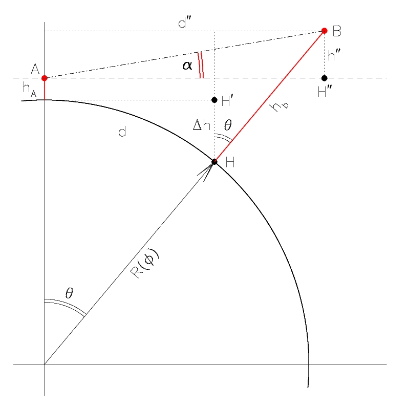
Figure 6: Geometry of the problem.