Utility Optimal Coding for Packet Transmission over Wireless Networks – Part II:
Networks of Packet Erasure Channels

Abstract

We define a class of multi–hop erasure networks that approximates a wireless multi–hop network. The network carries unicast flows for multiple users, and each information packet within a flow is required to be decoded at the flow destination within a specified delay deadline. The allocation of coding rates amongst flows/users is constrained by network capacity. We propose a proportional fair transmission scheme that maximises the sum utility of flow throughputs. This is achieved by jointly optimising the packet coding rates and the allocation of bits of coded packets across transmission slots.

I Introduction

In a communication network, the network capacity is shared by a set of flows. There is a contention for resources among the flows, which leads to many interesting problems. One such problem, is how to allocate the resources optimally across the (competing) flows, when the physical layer is erroneous. Specifically, schedule/transmit time for a flow is a resource that has to be optimally allocated among the competing flows. In this work, we pose a network utility maximisation problem subject to scheduling constraints that solve a resource allocation problem. In another work, we studied the problem of optimal resource allocation in networks [1].

Figure 1: An illustration of a wireless mesh network with 4 cells. Cells $a$, $b$, $c$, and $d$ use orthogonal channels CH₁, CH₂, CH₃, and CH₄ respectively. Nodes 3, 5, and 6 are bridge nodes. The bridge node 3 (resp. 5 and 6) is provided a time slice of each of the channels CH₁ & CH₂ (resp. CH₂ & CH₄ for node 5 and CH₂& CH₃& CH₄ for node 6). Three flows $f_{1},f_{2}$, and $f_{3}$ are considered. In this example, $\mathcal{C}_{f_{1}}=\{a,b\}$, $\mathcal{C}_{f_{2}}=\{d,b,a\}$, and $\mathcal{C}_{f_{3}}=\{c,d\}$.

We define a class of multi–hop erasure networks, and consider packet communication over this class. The network consists of a set of $C\geq 1$ cells $\mathcal{C}=\{1,2,\cdots,C\}$ which define the “interference domains” in the network. We allow intra–cell interference (i.e transmissions by nodes within the same cell interfere) but assume that there is no inter–cell interference. This captures, for example, common network architectures where nodes within a given cell use the same radio channel while neighbouring cells using orthogonal radio channels. Within each cell, any two nodes are within the decoding range of each other, and hence, can communicate with each other. The cells are interconnected using multi–radio bridging nodes to create a multi–hop wireless network. A multi–radio bridging node $i$ connecting the set of cells $\mathcal{B}(i)=\{c_{1},..,c_{n}\}\subset\mathcal{C}$ can be thought of as a set of $n$ single radio nodes, one in each cell, interconnected by a high–speed, loss–free wired backplane (see Figure 1).

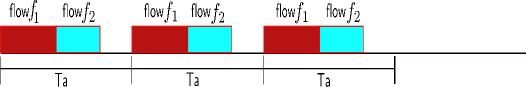
Figure 2: An illustration of transmission scheme in cell $a$ of the network in Figure 1: Every transmission schedule of $T_{a}$ time units is time–shared by nodes 1 and 3. Note that $\phi_{\Delta}(f)N_{f}R_{f}$ symbols of the encoded packet $p$ are transmitted in transmission schedule $p+\Delta$, where $\Delta\in\{0,1,2,\cdots,n_{f}-1\}$. The scheduling or capacity constraint of cell $a$ may not be tight (indicated by empty time slice in the figure), as the rates of flows $f_{1}$ and $f_{2}$ are governed by the whole network.

Data is transmitted across this multi–hop network as a set $\mathcal{F}$ $=$ $\{1,2,\cdots,F\}$, $F\geq 1$ of unicast flows. The route of each flow $f$ $\in\mathcal{F}$ is given by $\mathcal{C}_{f}$ $=$ $\{c_{1}(f),c_{2}(f),\cdots,c_{\ell_{f}}(f)\}$, where the source node $s(f)\in c_{1}(f)$ and the destination node $d(f)\in c_{\ell_{f}}(f)$. We assume loop–free flows (i.e., no two cells in $\mathcal{C}_{f}$ are same). Figures 1 and 2 illustrate this network setup. A scheduler assigns a time slice of duration $T_{f,c}>0$ time units to each flow $f$ that flows through cell $c$, subject to the constraint that $\sum_{f:c\in\mathcal{C}_{f}}T_{f,c}\leq T_{c}$ where $T_{c}$ is the period of the schedule in cell $c$. We consider a periodic scheduling strategy (see Figure 2) in which, in each cell $c$, service is given to the flows in a round robin fashion, and that each flow $f$ in cell $c$ gets a time slice of $T_{f,c}$ units in every schedule.

The scheduled transmit times for flow $f$ in source cell $c_{1}(f)$ define time slots for flow $f$. We assume that a new information packet arrives in each time slot, which allows us to simplify the analysis by ignoring queueing. Information packets of each flow $f$ at the source node $S(f)$ consist of a block of $k_{f}$ symbols. Each packet of flow $f$ is encoded into codewords of length $n_{f}=k_{f}/r_{f}$ symbols, with coding rate $0<{r_{f}}\leq 1$. The code employed for encoding is discussed in Section II. We require sufficient transmit times at each cell along route $\mathcal{C}_{f}$ to allow $n_{f}$ coded symbols to be transmitted in every schedule period. Hence there is no queueing at the cells along the route of a flow. It is not apparent at this point whether it is optimal for flow $f$ to transmit a single code–word of $n_{f}$ symbols or transmit a block of $n_{f}$ symbols where each block carries some portions of each of a set of coded packets.

Channel Model: The channel in cell $c$ for flow $f$ is considered to be a packet erasure channel with the probability of packet erasure being $\beta_{f,c}\in[0,1]$. Thus, the end–to–end channel for flow $f$ is a packet erasure channel with the probability of packet erasure being

$$\beta_{f}=1-\prod_{c\in\mathcal{C}_{f}}\left[1-\beta_{f,c}\right]$$

Let the Bernoulli random variable $E_{f}[i]$ indicate the end–to–end erasure seen by the $i$th block of flow $f$ (independent of the erasure seen by other blocks) of flow $f$. Note that $E_{f}[i]=1$ means that the $i$th block is erased, and $E_{f}[i]=0$ means that the $i$th block is received successfully. Note that ${\sf P}\{E_{f}[i]=1\}=\beta_{f}=1-{\sf P}\{E_{f}[i]=0\}$.

Each packet has a deadline of $D_{f}$ slots, by which time it must be decoded. Such a delay constraint is natural in applications such as video streaming. A packet is in error if the destination fails to decode the packet by the deadline. Letting $e_{f}(r_{f})$ denote the error probability that a packet fails to be decoded before its deadline, the expected number of information symbols successfully received is $S_{f}(r_{f})=k_{f}(1-e_{f}(r_{f}))$. Other things being equal, we expect that decreasing $r_{f}$ (i.e., increasing the number of coded symbols $n_{f}=k_{f}/r_{f}$ sent) decreases error probability $e_{f}$ and so increases $S_{f}$. However, since the network capacity is limited, and is shared by multiple flows, increasing the coded packet size $n_{f_{1}}$ of flow $f_{1}$ generally requires decreasing the packet size $n_{f_{2}}$ for some other flow $f_{2}$. That is, increasing $S_{f_{1}}$ comes at the cost of decreasing $S_{f_{2}}$. We are interested in understanding this trade–off, and in analysing the optimal fair allocation of coding rates amongst users/flows.

Our main contribution is the analysis of fairness in the allocation of coding rates between users/flows competing for limited network capacity. In particular, we adopt a utility–fair framework, and propose a scheme for obtaining the proportional fair allocation of coding rates, i.e. the allocation of coding rates that maximises $\sum_{f\in\mathcal{F}}\log S_{f}(r_{f})$ subject to network capacity constraints. This problem, which we show in Section III, requires solving a non–convex optimisation problem. Specifically, at the physical layer, the (channel) coding rate of a flow can be lowered (to alleviate its channel errors) only at the expense of increasing the coding rates of other flows. Also, at the network layer, the length of schedules of each flow should be chosen in such a way that it maximises the network utility. Interestingly, we show in our problem formulation that the coding rate and the scheduling are tightly coupled. Also, we show that for a $\log$ (network) utility function (which typically gives proportional fair allocation of resources) the optimum rate allocation (in general) gives unequal air–times which is quite different from the previously known result of proportional fair allocation being the same as that of equal air–time allocation ([2]). This problem, which we show in Section III, requires solving a non–convex optimisation problem. Our work differs from the previous work on network utility maximisation (see [3] and the references therein) in the following manner. To the best of our knowledge, this is the first work that computes the optimal coding rate for a given scheduling (or capacity) constraints in the utility–optimal framework.

The rest of the paper is organised as follows. In Section II, we obtain a measure for the end–to–end packet erasure, and describe the throughput of the network. We then formulate a network utility maximisation problem subject to constraints on the transmission schedule lengths. In Section III, we obtain the optimum transmission strategy and the optimum packet–level coding rates for each flow in the network. In Section V, we provide some simple examples to illustrate our results. Due to lack of space, the proofs of various Lemmas are omitted.

II Problem Formulation

The encoding has two stages. The first stage is the encoding of each information packet using a standard generator matrix such as a Reed–Solomon code or a fountain code [4]. Let $P_{f}[t]$ denote the information packet that arrives at the source of flow $f$ in slot $t$. A packet $P_{f}[t]$ of flow $f$ has $k_{f}$ symbols, the encoded packet $C_{f}[t]$ of which is of size $n_{f}=k_{f}/r_{f}$ with $0<r_{f}\leq 1$, and we assume that the code is such that the packet $P_{f}[t]$ can be reconstructed from any of its $k_{f}$ encoded symbols (this is possible, for example, by Reed–Solomon codes).

The second stage allocates the content of the encoded packet $C_{t}$ of the first stage across the transmitted packets. Each encoded packet is segmented into $D_{f}$ portions (where we recall that $D_{f}$ is the decoding deadline requirement for each packet of flow $f$), the size of the $\Delta$th portion being $\phi_{f}(\Delta)n_{f}$, where $\Delta\in\{0,1,\cdots,D_{f}-1\}$ and $0\leqslant\phi_{f}(\Delta)\leqslant 1$. At transmission slot $t$, a transmitted packet is assembled from the $\phi_{f}(0)$ portion of $C_{f}[t]$, the $\phi_{f}(1)$ portion of $C_{f}[t-1]$, and so on until the $\phi_{f}(D_{f}-1)$th portion of packet $C_{f}[t-D_{f}+1]$. This procedure is illustrated in Figure 3 for $n_{f}=3$. Note that the transmitted packet is of size $n_{f}$ symbols. To decode a packet $P_{f}[t]$ of flow $f$, we use the transmitted packets that are received during the transmission slots $t,t+1,\cdots,t+D_{f}-1$. Note that the conventional strategy of transmitting an encoded packet every transmission slot corresponds to the special case: $\phi_{f}(0)=1$ and $\phi_{f}(1)=\phi_{f}(2)=\cdots=\phi_{f}({D_{f}-1})=0$. We call the transmission scheme outlined above with general $\phi_{\cdot}(\Delta)$s a generalised block transmission scheme.

Figure 3: Two stage encoding (example of $D_{f}=3)$: information packet $P_{f}[1]$ of size $k_{f}$ is encoded to $C_{f}[1]$ of size $n_{f}=k_{f}/r_{f}$, the contents of which are allocated across subpackets $\phi_{0}C_{f}[1],\phi_{1}C_{f}[1],\phi_{2}C_{f}[1]$ across $3$ timeslots.

II-A Network Constraints on Coding Rate

Let $w_{f,c}$ be the PHY rate of transmission of flow $f$ in cell $c$. For each transmitted packet of flow $f$, each cell $c\in\mathcal{C}_{f}$ along its route must allocate at least $\frac{n_{f}}{w_{f,c}}$ units of time to transmit the packet (or encoded block). Let $\mathcal{F}_{c}:=\{f\in\mathcal{F}:c\in\mathcal{C}_{f}\}$ be the set of flows that are routed through cell $c$. We recall that the transmissions in any cell $c$ are scheduled in a TDMA fashion, and hence, the total time required for transmitting packets for all flows in cell $c$ is given by $\sum_{f\in\mathcal{F}_{c}}\frac{n_{f}}{w_{f,c}}$. Since, for cell $c$, the transmission schedule interval is $T_{c}$ units of time, the coding rates $r_{f}$ must satisfy the schedulability constraint $\sum_{f\in\mathcal{F}_{c}}\frac{n_{f}}{w_{f,c}}\leqslant T_{c}$.

II-B Error Probability – Upper bound

Lemma 1.

The end–to–end probability of a packet erasure for flow $f$ is bounded by

$$\hskip 19.91692pt\widetilde{e}_{f}$$

$$=\ \mathsf{P}\left\{\sum_{\Delta=0}^{D_{f}-1}\phi_{f}(\Delta)\frac{k_{f}}{r_{f}}E_{f}[\Delta]>n_{f}-k_{f}\right\}$$

$$\leq\ \exp\left(-\left[\theta_{f}(1-r_{f})-\sum_{\Delta=0}^{D_{f}-1}\ln\left(1-\beta_{f}+\beta_{f}e^{\theta_{f}\cdot\phi_{f}(\Delta)}\right)\right]\right)$$

$$=:\ e_{f}.$$

where $\theta_{f}>0$ is the Chernoff–bound parameter.

Let the random variable $\alpha_{f}[t]$ indicate whether packet $P_{f}[t]$ is successfully decoded or not, i.e.,

$$\alpha_{f}[t] = \left\{\begin{array}[]{ll}1,&\text{if packet $P_{f}[t]$ is decoded successfully}\\ 0,&\text{otherwise}.\end{array}\right.$$

We note here that the decoding errors for the successive packets are correlated, as each encoded packet overlaps with the transmission of previous $D_{f}-1$ packets and the successive $D_{f}-1$ packets. Hence, the sequence of random variables $\alpha_{f}[1],\alpha_{f}[2],\alpha_{f}[3],\cdots$ are correlated. But, the probability of any $\alpha_{f}[t]=0$ is upper bounded by Lemma 1.

III Network Utility Maximisation

For flow $f$, the total expected throughput as a result of transmitting $T\geq 1$ packets is given by

$$S_{f}(T)$$

$$= \sum_{(x_{1},x_{2},\cdots,x_{T})\in\{0,1\}^{T}}\left(\sum_{t=1}^{T}k_{f}x_{t}\right){\sf P}\left\{\alpha_{f}[t]=x_{t},t=1,2,\cdots,T\right\}$$

Note that the joint probability mass function ${\sf P}\left\{\alpha_{f}[t]=x_{t},t=1,2,\cdots,T\right\}$ is not a product–form distribution as the packet erasures $\alpha_{f}[t]$s are correlated. However, the above expectation can be written as

$$S_{f}(T) =\sum_{t=1}^{T}\ \sum_{x_{t}\in\{0,1\}}k_{f}x_{t}{\sf P}\left\{\alpha_{f}[t]=x_{t}\right\}$$

$$=T\cdot k_{f}\cdot(1-e_{f})$$

Thus, the (average expected) flow throughput is defined as

$$S_{f} =\lim_{T\to\infty}\frac{S_{f}(T)}{T}$$

$$=k_{f}\cdot(1-e_{f}).$$

We are interested in maximising the utility of the network which is defined as the sum utility of flow throughputs. We consider the log of throughput as the candidate for the utility function being motivated by the desirable properties like proportional fairness that it possesses.

We define the following notations: the Chernoff–bound parameters ${\bm{\theta}}:=[\theta_{f}]_{f\in\mathcal{F}}$, coding rates ${\bm{r}}:=[r_{f}]_{f\in\mathcal{F}}$, and the allocation of coded bits across transmission slots ${\bm{\Phi}}:=[{\bm{\phi}}_{f}]_{f\in\mathcal{F}}$ where ${\bm{\phi}}_{f}:=[\phi_{f}(0),\phi_{f}(1),\cdots,\phi_{f}(D_{f}-1)]$. Thus, we define the network utility as

$$\widetilde{U}\left({\bm{\Phi}},{\bm{\theta}},{\bm{r}}\right) := \sum_{f\in\mathcal{F}}\ln\left(k_{f}\left(1-e_{f}({\bm{\phi}}_{f},\theta_{f},r_{f})\right)\right)$$ (2)

$$=: \sum_{f\in\mathcal{F}}\ln\left(k_{f}\right)+U\left({\bm{\Phi}},{\bm{\theta}},{\bm{r}}\right)$$

The problem is to obtain the optimum coded bit allocation ${\bm{\Phi}}^{*}$, the optimum Chernoff–bound parameter ${\bm{\theta}}^{*}$, and the optimum coding rate ${\bm{r}}^{*}$ that maximises the network utility. Since, $k_{f}$, the size of information packets of each flow $f$ is given, maximising the network utility is equivalent to maximising $U({\bm{\Phi}},{\bm{\theta}},{\bm{r}}):=\sum_{f\in\mathcal{F}}\ln\left(1-e_{f}\right)$. Thus, we define the following problem

P1:
$\displaystyle\max_{{\bm{\Phi}},{\bm{\theta}},{\bm{r}}}\ \ \$ $\displaystyle U({\bm{\Phi}},{\bm{\theta}},{\bm{r}})$ subject to $\displaystyle\underset{f:c\in\mathcal{C}_{f}}{\sum}\frac{k_{f}}{r_{f}w_{f,c}}\leq T_{c},$ $\displaystyle\forall c\in\mathcal{C}$ (3) $\displaystyle\underset{\Delta=0}{\overset{D_{f}-1}{\sum}}\phi_{f}(\Delta)=1,$ $\displaystyle\forall f\in\mathcal{F}$ (4) $\displaystyle\phi_{f}(\Delta)\geq 0,$ $\displaystyle\forall f\in\mathcal{F},0\leq\Delta\leq D_{f}-1$ $\displaystyle\theta_{f}>0,$ $\displaystyle\forall f\in\mathcal{F}$ $\displaystyle r_{f}\leq\overline{\lambda}_{f}\,$ $\displaystyle\forall f\in\mathcal{F}$ $\displaystyle r_{f}\geq\underline{\lambda}_{f}\,$ $\displaystyle\forall f\in\mathcal{F}$

We note that the Eqn. (3) enforces the network capacity (or the network schedulability) constraint. The objective function $U({\bm{\Phi}},{\bm{\theta}},{\bf r})$ is separable in $({\bm{\phi}}_{f},\theta_{f},r_{f})$ for each flow $f$. Importantly, the component of utility function for each flow $f$ given by $\ln\left(1-e_{f}({\bm{\phi}}_{f},\theta_{f},r_{f})\right)$ is not jointly concave in $({\bm{\phi}}_{f},\theta_{f},r_{f})$. However, $\ln\left(1-e_{f}({\bm{\phi}}_{f},\theta_{f},r_{f})\right)$ is concave in each of $\phi_{f}(\cdot)$, $\theta_{f}$, and $r_{f}$. Hence, the network utility maximisation problem ${\bf P1}$ is not in the standard convex optimisation framework. Instead, we pose the following problem,

P2:
$\displaystyle\max_{{\bm{\Phi}}}\max_{\bm{\theta}}\max_{\bm{r}}$ $\displaystyle\sum_{f\in\mathcal{F}}\ln\left(1-e_{f}({\bm{\phi}}_{f},\theta_{f},r_{f})\right)$ (5) subject to $\displaystyle\underset{f:c\in\mathcal{C}_{f}}{\sum}\frac{k_{f}}{r_{f}w_{f,c}}\leq T_{c},$ $\displaystyle\forall c\in\mathcal{C}$ $\displaystyle\underset{\Delta=0}{\overset{D_{f}-1}{\sum}}\phi_{f}(\Delta)=1,$ $\displaystyle\forall f\in\mathcal{F}$ $\displaystyle\phi_{f}(\Delta)\geq 0,$ $\displaystyle\forall f\in\mathcal{F},0\leq\Delta\leq D_{f}-1$ $\displaystyle\theta_{f}>0,$ $\displaystyle\forall f\in\mathcal{F}$ $\displaystyle r_{f}\leq\overline{\lambda}_{f}\,$ $\displaystyle\forall f\in\mathcal{F}$ $\displaystyle r_{f}\geq\underline{\lambda}_{f}\,$ $\displaystyle\forall f\in\mathcal{F}$

In general, the solution to ${\bf P2}$ need not be the solution to ${\bf P1}$. However, in our problem, we show that ${\bf P2}$ achieves the solution of ${\bf P1}$.

Lemma 2.

. For a function $f:{\cal Y}\times{\cal Z}\to{\mathbb{R}}$ that is concave in $y$ and in $z$, but not jointly in $(y,z)$, the solution to the joint optimisation problem for convex sets ${\cal Y}$ and ${\cal Z}$
$\displaystyle\max_{y\in{\cal Y},z\in{\cal Z}}f(y,z)$ (6) is the same as
$\displaystyle\max_{z\in{\cal Z}}\max_{y\in{\cal Y}}f(y,z),$ (7)
if $f(y^{*}(z),z)$ is a concave function of $z$, where for each $z\in{\cal Z}$, $y^{*}(z):=\underset{y\in{\cal Y}}{\arg\max}f(y,z)$.

We note that for each $r_{f}$ and $\theta_{f}$, the probability of error $e_{f}$ is convex in ${{\bm{\phi}}_{f}}$, and hence, $\ln(1-e_{f})$ is concave in ${\bm{\phi}}_{f}$. Thus, we first solve for the optimum code bit allocation ${\bm{\phi}}^{*}_{f}$ in Section IV-A. Then, using the optimum code bit allocation, we solve for the optimum Chernoff bound parameter ${\bm{\theta}}^{*}$ which we describe in subsection IV-B. After having solved for the optimum ${\bm{\theta}}^{*}$, we show in Section IV-C that $U({\bm{\Phi}}^{*},{\bm{\theta}}^{*}({\bm{r}}),{\bm{r}})$ is a concave function of ${\bm{r}}$. Hence, from Lemma 2, the solution to problem $({\bf P2})$ (the maximisation problem that separately obtains the optimum ${\bm{\theta}}^{*}$ and optimum ${\bm{r}}^{*}$) is globally optimum. We study the rate optimisation problem that obtains ${\bm{r}}^{*}$ in subsection IV-D.

IV Utility Optimum Rate Allocation

IV-A Optimal Code Bit Allocation $\boldmath{\Phi}$

We consider the maximisation problem defined in Eqn. 5 for a given coding rate vector ${\bm{r}}$ and Chernoff–bound parameter vector ${\bm{\theta}}$, and obtain the optimum ${\bm{\phi}}_{f}$ for each flow $f\in\mathcal{F}$. The sub–problem is given by

$$\max_{{\bm{\phi}}_{f}} \sum_{f\in\mathcal{F}}\ln\left(1-e_{f}({\bm{\phi}}_{f},\theta_{f},r_{f})\right)$$

subject to $$\begin{array}[]{lllll}\underset{\Delta=0}{\overset{D_{f}-1}{\sum}}\phi_{f}(\Delta)&=&1,&\forall f\in\mathcal{F}&\\ \phi_{f}(\Delta)&\geq&0,&\forall f\in\mathcal{F},\forall\Delta\leq D_{f}-1.&\end{array}$$

This is a separable convex optimisation problem, and hence can be solved by Lagrangian method. Let $\mu_{f}$ be a Lagrangian multiplier for the constraint $\underset{\Delta=0}{\overset{D_{f}-1}{\sum}}\phi_{f}(\Delta)=1$, and define ${\bm{\mu}}=[\mu_{f}]_{f\in\mathcal{F}}$. The Lagrangian function is given by

$$L({\bf\Phi},\bm{\mu})=\sum_{f\in\mathcal{F}}\ln\left(1-e_{f}\right)-\sum_{f\in\mathcal{F}}\mu_{f}\bigg{(}1-\sum_{\Delta=0}^{D_{f}-1}\phi_{f}(\Delta)\bigg{)}$$

Applying KKT condition,

$$\frac{\partial L\hskip 11.38109pt}{\partial\phi_{f}(i)}\mid_{\phi_{f}(i)^{*}} = 0,$$

we get

$$0 = \frac{-e_{f}}{1-e_{f}}\cdot\frac{\beta_{f}\theta_{f}e^{\theta_{f}{\phi^{*}_{f}(i)}}}{1-\beta_{f}+\beta_{f}e^{\theta_{f}\phi^{*}_{f}(i)}}+\mu_{f}$$

$$\text{or},\ e^{\theta_{f}{\phi^{*}_{f}(i)}} = \frac{1-\beta_{f}}{\beta_{f}}\frac{(1-e_{f})\mu_{f}}{\theta_{f}e_{f}-\mu_{f}(1-e_{f})}$$ (9)

for $i=0,1,2,\cdots,n_{f}-1$. Since, the RHS of Eqn. IV-A is the same for all $i$, we get $\phi^{*}_{f}(i)=\phi^{*}_{f}(j)$, and hence

$$\phi^{*}_{f}(\Delta)=\frac{1}{D_{f}},\ \forall\Delta=0,1,\cdots,D_{f}-1.$$

Thus, ${\bf\Phi}^{*}$ allocates equal portions of an encoded packet across transmission schedules with a delay of $0,1,\cdots,D_{f}-1$, unlike the conventional transmission scheme which transmits all the coded bits of a packet in one shot. Hence, $e_{f}({\bm{\phi}}_{f}^{*},\theta_{f},r_{f})$ is

$$e_{f} =\exp\left(-\left[\theta_{f}(1-r_{f})-D_{f}\ln\left(1-\beta_{f}+\beta_{f}e^{\frac{\theta_{f}}{D_{f}}}\right)\right]\right).$$ (10)

IV-B Optimal $\boldmath{\theta}^{*}$

We now consider the optimum Chernoff–bound parameter problem with the optimum coded bits allocation ${\bm{\Phi}}^{*}$, and for any given coding rate vector ${\bm{r}}\in[\underline{\lambda}_{f},\overline{\lambda}_{f}]^{F}$.

$$\max_{\bm{\theta}} \sum_{f\in\mathcal{F}}\ln\left(1-e_{f}({\bm{\phi}}_{f}^{*},\theta_{f},r_{f})\right)$$ (11)

subject to $$\theta_{f}>0,\ \ \ \ \ \forall f\in\mathcal{F}$$

We note that the objective function is separable in $\theta_{f}$s, and that $e_{f}$ is convex in $\theta_{f}$. Hence, the problem defined in Eqn. (11), is a concave maximisation problem. The partial derivative of $e_{f}$ with respect to $\theta_{f}$ is given by

$$\frac{\partial e_{f}}{\partial\theta_{f}} =-e_{f}\cdot\left[(1-r_{f})-\frac{\beta_{f}e^{\theta_{f}/D_{f}}}{1-\beta_{f}+\beta_{f}e^{\theta_{f}/D_{f}}}\right].$$

Observe that $\frac{\beta_{f}e^{\theta_{f}/D_{f}}}{1-\beta_{f}+\beta_{f}e^{\theta_{f}/D_{f}}}$ is an increasing function of $\theta_{f}$. Thus, if, for $\theta_{f}=0$, $1-r_{f}-\frac{\beta_{f}}{1-\beta_{f}+\beta_{f}}<0$ or $r_{f}>1-\beta_{f}$, the derivative is positive for all $\theta_{f}>0$, or $e_{f}$ is an increasing function of $\theta_{f}$. Hence, for $r_{f}>1-\beta_{f}$, the optimum $\theta_{f}^{*}$ is arbitrarily close to $0$ which yields $e_{f}$ arbitrarily close to $1$. Thus, for error recovery, for any end–to–end error probability $\beta_{f}$, the coding rate should be smaller than $1-\beta_{f}$, in which case, we obtain the optimum $\theta_{f}^{*}$ by equating the partial derivative of $e_{f}$ with respect to $\theta_{f}$ to zero.

$$\begin{array}[]{lrcl}\text{i.e.,}&\frac{\beta_{f}e^{\theta_{f}^{*}/D_{f}}}{1-\beta_{f}+\beta_{f}e^{\theta_{f}^{*}/D_{f}}}&=&1-r_{f}\\ \text{or},&e^{\theta_{f}^{*}/D_{f}}&=&\frac{1-r_{f}}{\beta_{f}}\frac{1-\beta_{f}}{r_{f}}\\ \text{or},&\theta_{f}^{*}&=&D_{f}\left[\ln\left(\frac{1-r_{f}}{\beta_{f}}\right)-\ln\left(\frac{r_{f}}{1-\beta_{f}}\right)\right].\end{array}$$

Thus, the probability of a packet decoding error for a given $r_{f}$ with the optimum allocation of coded bits ${\bm{\Phi}}^{*}$, and the optimum Chernoff–bound parameter $\theta_{f}^{*}$, is

$$\ \ \ \ e_{f}$$

$$=\exp\left(-D_{f}\left[(1-r_{f})\ln\left(\frac{1-r_{f}}{\beta_{f}}\right)+r_{f}\ln\left(\frac{r_{f}}{1-\beta_{f}}\right)\right]\right)$$

$$=\exp\left(-D_{f}\cdot\text{KL}(\mathcal{B}(1-r_{f})||\mathcal{B}(\beta_{f})\right)$$

where KL$(f_{1},f_{2})$ is the Kullback–Leibler divergence between the probability mass functions (pmfs) $f_{1}$ and $f_{2}$.

IV-C A convex optimisation framework to obtain optimal $r_{f}^{*}$

If $\ln(1-e_{f}({\bm{\phi}}^{*}_{f},\theta_{f}^{*},r_{f}))$ is concave in $r_{f}$, then one can obtain the optimum $r_{f}^{*}$ using convex optimisation framework. To show the concavity of $\ln(1-e_{f}({\bm{\phi}}^{*}_{f},\theta_{f}^{*},r_{f}))$ it is sufficient to show that $e_{f}({\bm{\phi}}^{*}_{f},\theta_{f}^{*},r_{f})$ is convex in $r_{f}$. Note that

$$\frac{\partial e_{f}}{\partial r_{f}} =e_{f}\cdot\theta_{f}^{*}(r_{f})$$

$$\frac{\partial^{2}e_{f}}{\partial r_{f}^{2}} ={e_{f}}\left[\theta_{f}^{*2}-\frac{D_{f}}{r_{f}(1-r_{f})}\right]$$

$e_{f}$ is convex if

$$\left[\ln\left(\frac{1-r_{f}}{\beta_{f}}\right)-\ln\left(\frac{r_{f}}{1-\beta_{f}}\right)\right]^{2} \geq\frac{D_{f}}{r_{f}(1-r_{f})},$$

or,

$$\ln\left(\frac{1-r_{f}}{r_{f}}\frac{1-\beta_{f}}{\beta_{f}}\right) \geq\frac{\sqrt{D_{f}}}{\sqrt{r_{f}(1-r_{f})}}$$

$$\text{or},\ \frac{\sqrt{D_{f}}}{\sqrt{r_{f}(1-r_{f})}}-\ln\left(\frac{1-r_{f}}{r_{f}}\frac{1-\beta_{f}}{\beta_{f}}\right) \leq 0$$

The function $\frac{1}{\sqrt{r_{f}(1-r_{f})}}$ is convex in $r_{f}$. Also, $\ln\left(\frac{1-r_{f}}{r_{f}}\right)$ is decreasing with $r_{f}$, and hence, $-\ln\left(\frac{1-r_{f}}{r_{f}}\frac{1-\beta_{f}}{\beta_{f}}\right)\leq-\ln\left(\frac{1-\overline{\lambda}_{f}}{\overline{\lambda}_{f}}\frac{1-\beta_{f}}{\beta_{f}}\right)$. Thus, we have a sufficient condition

$$\frac{\sqrt{D}_{f}}{\sqrt{r_{f}(1-r_{f})}}-\ln\left(\frac{1-\overline{\lambda}_{f}}{\overline{\lambda}_{f}}\frac{1-\beta_{f}}{\beta_{f}}\right) \leq 0$$ (12)

The above condition requires the delay deadline $D_{f}$ to be smaller than some $\overline{D}_{f}(r_{f})$. We consider $D_{f}$s to satisfy this condition, and hence, the rate optimisation problem is a concave maximisation problem. For the sake of completeness, we include this as a constraint in the problem formulation. However, this condition is not an active constraint.

IV-D Optimal Coding Rate $\boldmath{r}$

From the previous subsection, we observe under the delay constraint Eqn. (12) that $e_{f}({\bm{\phi}}^{*}_{f},\theta_{f}^{*}(r_{f}),r_{f})$ is convex in $r_{f}$, and hence, we obtain the optimum coding rate $r_{f}^{*}$ using convex optimisation method. Also, from Lemma 2, it is clear that $r_{f}^{*}$ is the unique globally optimum rate. Thus, we solve the following network utility maximisation problem
$\displaystyle\max_{\bm{r}}$ $\displaystyle\sum_{f\in\mathcal{F}}\ln\left(1-e_{f}({\bm{\phi}}^{*}_{f},\theta_{f}^{*}(r_{f}),r_{f})\right)$ (13) subject to $\displaystyle\underset{f:c\in\mathcal{C}_{f}}{\sum}\frac{k_{f}}{r_{f}w_{f,c}}\leq T_{c},$ $\displaystyle\forall c\in\mathcal{C}$ $\displaystyle r_{f}\leq\overline{\lambda}_{f}\,$ $\displaystyle\forall f\in\mathcal{F}$ $\displaystyle r_{f}\geq\underline{\lambda}_{f}\,$ $\displaystyle\forall f\in\mathcal{F}$ $\displaystyle\frac{\sqrt{D_{f}}}{\sqrt{r_{f}(1-r_{f})}}-a\leq 0\,$ $\displaystyle\forall f\in\mathcal{F}$ (14)
where $a=\ln\left(\frac{1-\overline{\lambda}_{f}}{\overline{\lambda}_{f}}\frac{1-\beta_{f}}{\beta_{f}}\right)$. It is clear that the objective function is separable and concave, and hence, can be solved using Lagrangian relaxation method. Also, we note here that the constraint represented by Eqn. (14) is not an active constraint, and hence, there is no Lagrangian cost to this constraint. We note here that the coding rate should be such that $k_{f}/r_{f}$ is an integer, and hence, obtaining $r_{f}^{*}$ is a discrete optimisation problem. This is, in general, an NP hard problem. Hence, we relax this constraint, and allow $r_{f}$ to take any real value in $[\underline{\lambda}_{f},\overline{\lambda}_{f}]$. The Lagrangian function for the rate optimisation problem is thus

$$\ \ \ \ L({\bm{r}},{\bm{p}},{\bm{u}},{\bm{v}})$$

$$=\sum_{f\in\mathcal{F}}\ln\left(1-e_{f}\right)-\sum_{c\in\mathcal{C}}p_{c}\left(\sum_{f\in\mathcal{F}_{c}}\frac{k_{f}}{r_{f}w_{f,c}}-T_{c}\right)$$

$$+\sum_{f\in\mathcal{F}}u_{f}\left(r_{f}-\underline{\lambda}_{f}\right)-\sum_{f\in\mathcal{F}}v_{f}\left(r_{f}-\overline{\lambda}_{f}\right)$$

Applying KKT condition, $\frac{\partial L}{\partial r_{f}}\mid_{r_{f}^{*}}=0$, we have

$$\frac{-1}{1-e_{f}}\frac{\partial e_{f}}{\partial r_{f}}\mid_{r_{f}^{*}} =\sum_{c\in\mathcal{C}_{f}}p_{c}\frac{-k_{f}}{r_{f}^{*2}w_{f,c}}+v_{f}-u_{f}$$

$$=\frac{-k_{f}}{r_{f}^{*2}}\left(\sum_{c\in\mathcal{C}_{f}}\frac{p_{c}}{w_{f,c}}\right)+v_{f}-u_{f}$$

$$\frac{e_{f}}{1-e_{f}}\cdot\theta_{f}^{*} =\frac{k_{f}}{r_{f}^{*2}}\left(\sum_{c\in\mathcal{C}_{f}}\frac{p_{c}}{w_{f,c}}\right)+v_{f}-u_{f}.$$

If the optimum $r_{f}^{*}$ is either $\underline{\lambda}_{f}$ or $\overline{\lambda}_{f}$, then it is unique. If $r_{f}^{*}\in(\underline{\lambda}_{f},\overline{\lambda}_{f})$, then $u_{f}=v_{f}=0$, which is the most interesting case, and we consider only this case for the rest of the paper. Let $\lambda_{f}:=\sum_{c\in\mathcal{C}_{f}}\frac{p_{c}}{w_{f,c}}$. The above equation becomes

$$\frac{e_{f}}{1-e_{f}}\cdot\theta_{f}^{*} =\frac{\lambda_{f}k_{f}}{r_{f}^{*2}}$$ (15)

$$e_{f} =\frac{\lambda_{f}k_{f}}{\lambda_{f}k_{f}+\theta_{f}^{*}r_{f}^{*2}}$$ (16)

$$\exp\left(-D_{f}D({\cal B}(1-r^{*}_{f})\|{\cal B}(\beta_{f}))\right) =\frac{\lambda_{f}k_{f}}{\lambda_{f}k_{f}+\theta_{f}^{*}r_{f}^{*2}}$$

$$D_{f}D({\cal B}(1-r_{f}^{*})\|{\cal B}(\beta_{f})) =\ln\left(\frac{\lambda_{f}k_{f}+\theta_{f}^{*}r_{f}^{*2}}{\lambda_{f}k_{f}}\right)$$ (17)

In the above equation, the LHS is a strictly convex decreasing function of $r_{f}^{*}$. Since, the utility maximisation problem is a concave maximisation problem, the optimum rate $r_{f}^{*}\in(0,1-\beta_{f})$ exists and is unique.

IV-E Sub–gradient Approach to Compute optimum ${p}_{c}^{*}$

In this section, we discuss the procedure to obtain the Shadow costs or the Lagrange variables ${\bm{p}}^{*}$. The dual problem for the primal problem defined in Eqn. (13) is given by

$$\min_{{\bm{p}}\geq 0} D(\bm{p}),$$

where the dual function $D(\bm{p})$ is given by

$$\hskip 14.22636ptD(\bm{p})$$

$$=\max_{{\bm{r}}}\underset{f\in\mathcal{F}}{\sum}\ln(1-e_{f}(r_{f}))+\underset{c\in\mathcal{C}}{\sum}p_{c}\left(T_{c}-\underset{f\in\mathcal{F}_{c}}{\sum}\frac{k_{f}}{r_{f}w_{f,c}}\right)$$ (18)

$$=\underset{f\in\mathcal{F}}{\sum}\ln(1-e_{f}(r_{f}^{*}({\bm{p}})))+\underset{c\in\mathcal{C}}{\sum}p_{c}\left(T_{c}-\underset{f\in\mathcal{F}_{c}}{\sum}\frac{k_{f}}{r_{f}^{*}({\bm{p}})w_{f,c}}\right).$$ (19)

In the above equation, $e_{f}(r_{f})$ denotes $e_{f}({\bm{\phi}}^{*}_{f},\theta_{f}^{*}(r_{f}),r_{f})$. Since the dual function (of a primal problem) is convex, $D$ is convex in ${\bm{p}}$. Hence, we use a sub–gradient method to obtain the optimum $\bm{p}^{*}$. From Eqn. (18), it is clear that for any ${\bm{r}}$,

$$D(\bm{p}) \geq\underset{f\in\mathcal{F}}{\sum}\ln(1-e_{f}(r_{f}))+\underset{c\in\mathcal{C}}{\sum}p_{c}\left(T_{c}-\underset{f\in\mathcal{F}_{c}}{\sum}\frac{k_{f}}{r_{f}w_{f,c}}\right),$$

and in particular, $D({\bm{p}})$ is greater than that for $r=r_{f}^{*}({\widetilde{\bm{p}}})$, i.e.,

$$\hskip 14.22636ptD(\bm{p})$$

$$\geq\underset{f\in\mathcal{F}}{\sum}\ln(1-e_{f}(r_{f}^{*}({\widetilde{\bm{p}}})))+\underset{c\in\mathcal{C}}{\sum}p_{c}\left(T_{c}-\underset{f\in\mathcal{F}_{c}}{\sum}\frac{k_{f}}{r_{f}^{*}({\widetilde{\bm{p}}})w_{f,c}}\right)$$

$$=D(\widetilde{\bm{p}})+\underset{c\in\mathcal{C}}{\sum}\left(p_{c}-\widetilde{p}_{c}\right)\left(T_{c}-\underset{f\in\mathcal{F}_{c}}{\sum}\frac{k_{f}}{r_{f}^{*}({\widetilde{\bm{p}}})w_{f,c}}\right)$$ (20)

Thus, a sub–gradient of $D(\cdot)$ at any $\widetilde{\bm{p}}$ is given by the vector

$$\left[T_{c}-\underset{f\in\mathcal{F}_{c}}{\sum}\frac{k_{f}}{r_{f}^{*}({\widetilde{\bm{p}}})w_{f,c}}\right]_{c\in\mathcal{C}}.$$ (21)

We obtain an iterative algorithm based on sub–gradient method that yields $\bm{p}^{*}$, with ${\bm{p}}(i)$ being the Lagrangians at the $i$th iteration.

$$p_{c}(i+1)=\left[p_{c}(i)-\gamma\cdot\left(T_{c}-\underset{f\in\mathcal{F}_{c}}{\sum}\frac{k_{f}}{r_{f}^{*}({\bm{p}}(i))w_{f,c}}\right)\right]^{+}.$$

where $\gamma>0$ is a sufficiently small stepsize, and $[f(x)]^{+}:=\max\{f(x),0\}$ ensures that the Lagrange multiplier never goes negative. Note that the Lagrangian updates can be locally done, as each cell $c$ is required to know only the rates $r_{f}^{*}({\bm{p}}(i))$ of flows $f\in\mathcal{F}_{c}$. Thus, at the beginning of each iteration $i$, the flows choose their coding rates to $r_{f}^{*}({\bm{p}}(i))$, and each cell computes its cost based on the rates of flows through it. The updated costs along the route of each flow are then fed back to the source node to compute the rate for the next iteration.

The Lagrange multiplier $p_{c}$ can be viewed as the cost of transmitting traffic through cell $c$. The amount of service time that is available is given by $\delta=T_{c}-\underset{f\in\mathcal{F}_{c}}{\sum}\frac{k_{f}}{r_{f}^{*}({\bm{p}}(i))w_{f,c}}$. When $\delta$ is positive and large, then the Lagrangian cost $p_{c}$ decreases rapidly (because $D$ is convex), and when $\delta$ is negative, then the Lagrangian cost $p_{c}$ increases rapidly to make $\delta\geq 0$. We note that the increase or decrease of $p_{c}$ between successive iterations is proportional to $\delta$, the amount of service time available. Thus, the sub–gradient procedure provides a dynamic control scheme to balance the network loads.

We explore the properties of the optimum rate parameter $r_{f}^{*}$ in Section IV-F. In Section V, we provide some examples that illustrate the optimum utility–fair resource allocation.

IV-F Properties of $r_{f}^{*}$

Lemma 3.

$r_{f}^{*}(D_{f})$ is an increasing function of $D_{f}$.

Lemma 3 is quite intuitive. For any given channel error $\beta_{f}$, as the deadline become less stringent, it is optimal to go for a high rate code. In other words, it is optimal for a flow to use as much scheduling time as possible (for a large $D_{f}$, and hence, use a high rate code); however, the resources are shared among multiple flows, and hence, we ask the following question: “what is the optimal share of the scheduling time” that each flow should have. Interestingly, in our problem formulation, the code rate $r_{f}$ also solves this optimal scheduling times for each flows.

V Examples

V-A Example 1: Two cells with equal traffic load

We begin by considering the example shown in Figure 4 consisting of two cells $a$ and $b$ having three nodes 1, 2, and 3. Each cell has the same packet erasure probability $\beta$ and the schedule length $T$. There are three flows $f_{1},f_{2}$, and $f_{3}$, with two of the flows $f_{1}$ and $f_{3}$ having one–hop routes $\mathcal{C}_{f_{1}}=\{b\}$ and $\mathcal{C}_{f_{3}}=\{a\}$, and one flow $f_{2}$ having a two–hop route $\mathcal{C}_{f_{2}}=\{a,b\}$. Each flow has the same information packet size $k$, decoding deadline $D$ and PHY transmit rate, i.e. $w_{f,c}=w$. This is analogous to the so–called parking–lot topology often used to explore fairness issues.

The end–to–end erasure probability experienced by the two–hop flow $f_{2}$ is greater than that experienced by the one hop flows $f_{1}$ and $f_{3}$, since each hop has the same fixed erasure probability. Hence, we need to assign a lesser coding rate $r_{f_{2}}$ to flow $f_{2}$ than to flows $f_{1}$ and $f_{3}$ in order to obtain the same error probability (after decoding) across flows. However, when operating at the boundary of the network capacity region (thereby maximising throughput), decreasing the coding rate $r_{f_{2}}$ of the two–hop flow $f_{2}$ requires that the coding rate of both one–hop flows $f_{1}$ and $f_{3}$ be increased in order to remain within the available network capacity. In this sense, allocating coding rate to the two–hop flow $f_{2}$ imposes a greater marginal cost on the network (in terms of the sum–utility) than the one–hop flows, and we expect that a fair allocation will therefore assign higher coding rate to the two–hop flow $f_{2}$. The solution optimising this trade–off in a proportional fair manner can be understood using the analysis in the previous section.

In this example, both the cells are equally loaded and, by symmetry, the Lagrange multipliers $p_{a}=p_{b}$. Hence, $\lambda_{f_{1}}=\frac{\lambda_{f_{2}}}{2}=\lambda_{f_{3}}$. For the Chernoff–bound parameter ${\bm{\theta}}=[\theta,\theta]$, we find from Eqn. (15),

$$\frac{e_{f_{2}}}{1-e_{f_{2}}}\cdot\frac{1-e_{f_{1}}}{e_{f_{1}}} = \frac{\lambda_{f_{2}}}{\lambda_{f_{1}}}\cdot\frac{r_{f_{1}}^{*2}}{r_{f_{2}}^{*2}}$$

$$= 2\cdot\frac{r_{f_{1}}^{*2}}{r_{f_{2}}^{*2}}.$$

For sufficiently small erasure probabilities, we have

$$\frac{e_{f_{2}}}{e_{f_{1}}} \approx 2\cdot\frac{r_{f_{1}}^{*2}}{r_{f_{2}}^{*2}}$$

$$\approx 2$$

Thus the proportional fair allocation is $e_{f_{1}}=e_{f_{3}}\approx 1/2\cdot e_{f_{2}}$. That is, the coding rates are allocated such that the one–hop flows have approximately half the error probability of the two–hop flow.

Figure 4: Cells with equal traffic load

V-B Example 2: Two cells with unequal traffic load

We consider the same network as in the previous example, but now with only the flows $f_{1}$ and $f_{2}$ (i.e., the flow $f_{3}$ is not present) in the network. In this example, cell b carries two flows while cell a carries only one flow. The encoding rate constraints are given by

$$\frac{1}{r_{f_{2}}} \leq \frac{wT}{k},\ \text{(from cell 1)},$$

$$\frac{1}{r_{f_{1}}}+\frac{1}{r_{f_{2}}} \leq \frac{wT}{k},\ \text{(from cell 2)}.$$

Since, both $r_{f_{1}}$ and $r_{f_{2}}$ are at most 1, it is clear that at the optimal point, the rate constraint of cell a is not tight while the constraint of cell b is tight. Thus, the shadow prices (Lagrange multipliers) $p_{a}=0$ and $p_{b}>0$. That is, at the first hop the cell is not operating at capacity, and so the “price” for using this cell is zero. In this example, $\lambda_{f_{1}}=\lambda_{f_{2}}$, and hence, from Eqn. (15), we deduce that for sufficiently low cell erasure probability $\beta$, $e_{f_{1}}\approx e_{f_{2}}$. Alternatively, as the delay deadline $D\to\infty$, from Eqn. (15) we have $e_{f_{1}}=e_{f_{2}}$. These proportional fair allocations make sense intuitively since although flow $f_{2}$ crosses two hops, it is only constrained at the second hop and so it is natural to share the available capacity of this second hop approximately equally between the flows. When the erasure probability is sufficiently small, this yields approximately the same error probabilities for both flows. For larger erasure probabilities, it leads to the two–hop flow having higher error probability, in proportion to the per–hop erasure probability $\beta$.

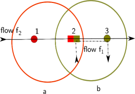
Figure 5: Cells with unequal traffic load

References

• [1] K. Premkumar, X. Chen, and D. J. Leith, “Utility optimal coding for packet transmission over wireless networks – Part I: Networks of binary synchronous channels,” in submitted, 2011.
• [2] A. Checco and D. J. Leith, “Proportional fairness in 802.11 wireless lans,” to appear in IEEE Comm. Letters, 2011.
• [3] S. Shakkottai and R. Srikant, Network Optimization and Control.   Now Publishers Inc., Boston - Delft, 2008.
• [4] A. Shokrollahi, “Raptor codes,” Information Theory, IEEE Transactions on, vol. 52, no. 6, pp. 2551 –2567, Jun. 2006.