The Next Generation Atlas of Quasar Spectral Energy Distributions from Radio to X-rays

Abstract

We have produced the next generation of quasar spectral energy distributions (SEDs), essentially updating the work of Elvis et al. (1994) by using high-quality data obtained with several space and ground-based telescopes, including NASA’s Great Observatories. We present an atlas of SEDs of 85 optically bright, non-blazar quasars over the electromagnetic spectrum from radio to X-rays. The heterogeneous sample includes 27 radio-quiet and 58 radio-loud quasars. Most objects have quasi-simultaneous ultraviolet-optical spectroscopic data, supplemented with some far-ultraviolet spectra, and more than half also have Spitzer mid-infrared IRS spectra. The X-ray spectral parameters are collected from the literature where available. The radio, far-infrared, and near-infrared photometric data are also obtained from either the literature or new observations. We construct composite spectral energy distributions for radio-loud and radio-quiet objects and compare these to those of Elvis et al., finding that ours have similar overall shapes, but our improved spectral resolution reveals more detailed features, especially in the mid and near-infrared.

1 INTRODUCTION

The supermassive black holes powering quasars (or active galactic nuclei (AGN)) do not themselves shine. It is the heated material surrounding the black holes that emits the radiation signatures of quasars. These signatures include broad emission lines characteristic of high-velocity gas moving at thousands of kilometers per second, and extremely high continuum luminosity in excess of that of entire galaxies. Continuum emission is seen in all parts of the electromagnetic spectrum from the highest energies (gamma rays and X-rays) to the lowest (radio waves). The power emitted is similarly high, within an order of magnitude or so, over much of this range, although there can be significant variation from quasar to quasar.

There are no single states of matter or single processes capable of reproducing the spectral energy distribution (SED) of a quasar. A combination of both thermal and non-thermal processes has been invoked to explain, at different parts of the SED, the emission from gas in a variety of states, at a variety of temperatures, at a variety of distances, and experiencing a variety of environments. Quasars seem to have many different components that are expressed in different parts of the electromagnetic spectrum.

So what are the components of the quasar? The central supermassive black hole is the ultimate engine, allowing the liberation of gravitational potential energy. The primary source of electromagnetic emission is likely an accretion disk formed of hot gas spiraling into the black hole and shining in the optical through ultraviolet (UV). A hot atmosphere upscatters the disk photons to X-ray energies. A jet shooting out from the inner accretion disk emits synchrotron radiation, dominating radio emission and sometimes higher energies. An obscuring torus of relatively cool gas and dust, heated by photons from the accretion disk, thermally radiates in the near-infrared (NIR) and mid-infrared (MIR). The far-infrared (FIR) part of the SED comes from cooler dust, perhaps distributed throughout the host galaxy, that may be heated by stars rather than the quasar itself. Other regions in and among these continuum-emitting parts are responsible for the prominent emission lines present in quasar spectra. The details of all these parts, mechanisms, and their relationships are not yet completely understood, because multi-wavelength data to further our understanding have been difficult to gather.

Multiwavelength astronomy is challenging. No single telescope can observe at all wavelengths. Many parts of the electromagnetic spectrum cannot penetrate the Earth’s atmosphere and require space-based observations. Quasars are variable and this means that simultaneous or nearly simultaneous observations are desirable, at least in some parts of the spectrum. Different technologies have different sensitivity levels and what may be an easily observed target at one wavelength may be difficult to detect at another.

There were a number of pioneering works on quasar SEDs in the 1980s (e.g., Edelson & Malkan, 1986; Ward et al., 1987; Kriss, 1988; Sanders et al., 1989; Sun & Malkan, 1989). In the 1990s, Elvis et al. (1994, hereafter E94) established the first large, high-quality atlas of quasar SEDs. The timing of their work was predicated on the launch of several space-based telescopes, notably IRAS in the mid to far infrared, IUE in the UV, and Einstein in the X-rays, that for the first time provided observations of large numbers of quasars in these wavebands. They established the differences between the SEDs of radio-loud (RL) and radio-quiet (RQ) quasars. They also characterized the variance of quasar SEDs, which is rather substantial, and explored the problem of bolometric corrections.

Since the work of E94, there have been several significant investigations of quasar SEDs (e.g., Kuraszkiewicz et al., 2003; Risaliti & Elvis, 2004). Richards et al. (2006) is the largest that covers the entire electromagnetic spectrum, including data from the Sloan Digital Sky Survey and Spitzer, supplemented by near-IR, GALEX ultraviolet, VLA radio, and ROSAT X-ray data, where available. One of their key findings was again the wide range of SED shapes, and how assuming a mean SED can potentially lead to errors in bolometric luminosities as high as 50%.

Other investigations of SEDs have focused on subclasses, like broad absorption line (BAL) quasars (e.g., Gallagher et al., 2007), 2MASS red quasars (Kuraszkiewicz et al., 2009), hard X-ray selected quasars (Polletta et al., 2000, 2007), or on individual objects (e.g., Zheng et al., 2001). More detailed SED work has been done on limited portions of the entire electromagnetic spectrum, such as the optical-X-ray (e.g., Laor et al., 1997), the FIR to optical (e.g., Netzer et al., 2007), or optical/UV to X-ray (Grupe et al., 2010).

There has also been work looking for relationships among more detailed spectral features, like emission lines and SEDs. Wilkes et al. (1999), examining 41 quasars with SED information, for instance, found a variety of Baldwin effects (Baldwin 1977), anticorrelations between emission-line equivalent width and UV luminosity, as well as some correlations between properties of Fe II and C IV emission lines and the ratio of the optical to X-ray luminosity. Schweitzer et al. (2006) and Netzer et al. (2007) studied Palomar-Green quasars with FIR to optical data and confirmed that most FIR radiation is due to star-forming activity. However, Netzer et al. (2007) also argue, based on a correlation between $L(5100\mbox{\AA})$ and $L(60\micron)$, an alternative view that a large fraction of FIR radiation could result from direct AGN heating.

Ideally what one would like in studying quasars is a complete inventory over all time and all directions of all photons emitted. The best we can do now is to obtain spectrophotometric snapshots, close in time, of some spectral regions, supplemented by photometry in other accessible wavebands, from our particular line of sight toward a quasar. The technology has improved since the 1990s, with spacecraft such as HST, Chandra and XMM, and Spitzer replacing IUE, Einstein and ROSAT, and IRAS, respectively.

This atlas is meant to update the last decade’s work with a modern set of quasar SEDs using the next generation of telescopes and instruments. Whenever possible we have striven to use high-quality spectrophotometry in addition to photometry, which will enable investigations like those of Wilkes et al. (1999). One hope is that spectral features will be found that correlate with SEDs and allow their shapes to be determined without the need for complete multi-wavelength observations. Any correlations found should provide deeper insight into quasars. We plan additional papers based on this data set performing various types of investigations, as well as addressing both observational and theoretical aspects of bolometric corrections.

In the next section (§2), we describe our sample, which is composed of three subsamples that have excellent quasi-simultaneous optical through UV or far-UV (FUV) spectrophotometry serving as a starting point for SED construction. We then describe the sample properties. Subsequent sections describe the data (§3), starting with about 100 MHz radio and moving to higher energies to about 10 keV X-ray. We then discuss corrections to the SEDs, such as Galactic dereddening and host galaxy removal (§4). In §5, we present the SEDs for our quasars individually, then as composites for radio-loud and radio-quiet subsamples, which are known to differ significantly. We then discuss the properties of the SEDs, and compare our composites with those of E94. We finish this paper with a summary of these results, future plans, and some concluding remarks (§6).

2 SAMPLE

In the past, in order to study the optical and ultraviolet properties of quasars, we embarked on several programs of obtaining quasi-simultaneous spectrophotometry utilizing various ground and space-based telescopes. As this is a challenging endeavor, and the data we obtained were of high quality, we began the construction of SEDs with these samples, adding data at longer and shorter wavelengths. For convenience, we refer to our three subsamples by the abbreviations PGX, FUSE-HST, and RLQ. These subsamples are described below, and Table The Next Generation Atlas of Quasar Spectral Energy Distributions from Radio to X-rays provides our combined SED sample of 85 objects and their basic properties.

Several objects in the FUSE-HST subsample are also in the other two subsamples and there may be repeated observations in UV and/or optical. We choose to analyze the data with the FUSE-HST subsample because of their higher quality.

2.1 PGX

The “PGX” sample consists of 22 of 23 Palomar-Green quasars in the complete sample selected by Laor et al. (1994, 1997) from the Bright Quasar Survey (BQS; Schmidt & Green, 1983). Interested in observing the soft-X-ray regime using bright quasars, Laor et al. (1994, 1997) started with the ultraviolet-excess selected BQS and added the restrictions that $z\leq 0.4$ and Galactic H i column density $N_{\rm HI}<1.9\times 10^{20}{\rm cm}^{-2}$. We obtained low-resolution ultraviolet spectra with HST and conducted quasi-simultaneous ground-based observations at McDonald Observatory, usually within a month. Shang et al. (2007) provide additional details and constructed the UV-optical SEDs for this sample.

2.2 FUSE-HST

The “FUSE-HST” sample originates with the FUSE AGN program (Kriss, 2000), which surveyed more than 100 of the UV-brightest AGNs. About 20 of these were also observed in an HST spectral snapshot survey with sufficient signal-to-noise ratio during 1999–2000. The FUSE observations were scheduled as close in time as possible with the HST snapshot observations, and ground-based optical spectra were also obtained during the same period at Kitt Peak National Observatory (KPNO). We exclude a few objects because of the lack of an optical spectrum (NGC 3783, low declination), very strong host galaxy contamination (NGC 3516), or strong variability (NGC 5548, also no simultaneous HST spectrum). Our final FUSE-HST sample includes 17 objects with quasi-simultaneous spectrophotometry extending to the FUV and covering rest wavelength from 900–9000 Å. This is a heterogeneous sample with low redshift ($z<0.5$). Shang et al. (2005) provides additional details.

2.3 RLQ

The “RLQ” sample originates with an early HST program to observe a large sample of radio-loud quasars selected to have a small range in extended radio luminosity, a property thought to be isotropic. Limitations of HST discovered after launch required adjustments to the sample and brighter objects were substituted for fainter ones. Over the course of four cycles, HST targeted nearly 50 quasars. Quasi-simultaneous optical spectrophotometry was obtained at several observatories, primarily McDonald Observatory and KPNO. Wills et al. (1995) and Netzer et al. (1995) provide additional details of the sample. A number of the radio-core dominant quasars are blazars, with optically violent variability due to synchrotron emission from a beamed jet. We have excluded these blazars from the sample based on rapid optical variability as we regard this component as a major complication in determining intrinsic and uniform SEDs for comparison.

2.4 Sample Properties

In order to summarize the properties of the combined sample, we have plotted some histograms (Fig. 1). We have distinguished radio-loud and radio-quiet quasars using radio-loudness calculated with our data. We have also measured the redshift and 3000 Å rest-frame continuum luminosity of the sample. Details are provided in §4.3.

Of the 85 objects in the final sample, there are 27 RQ and 58 RL quasars. All RQ quasars are from either PGX or FUSE-HST subsamples, having redshift less than 0.5. Most RL quasars are from the RLQ subsample and more than half of the RL quasars have redshift larger than 0.5.

Both RL and RQ samples span about 2 orders of magnitude in luminosity. The RL sample has an average luminosity about 6 times higher. These properties reflect the original selections of the subsamples.

We emphasize that as a whole, this sample is representative of UV/optical-bright quasars, both radio-loud and radio-quiet, but is not statistically complete or well-matched. Particular subsamples may be appropriate for general statistical studies and comparisons only if care is taken in their selection.

3 DATA

We collected both photometry and spectroscopy data for this work. Many data were obtained with space telescopes, including HST, FUSE, Spitzer, Chandra, and XMM. This ensures the unprecedented quality of the SEDs. Figure 2 shows two examples of our objects, marked with wavebands and instruments used to obtain the data. These will be discussed in detail in the following sections.

Most of the data were obtained between 1991 and 2007 except for some archival radio data which were obtained much earlier (see Table The Next Generation Atlas of Quasar Spectral Energy Distributions from Radio to X-rays for details). However, the problem of AGN intrinsic variability can be neglected statistically for the SED work, especially with regard to some portions (e.g., infrared) which have only very long timescale variation. Moreover, the FUV-UV-optical spectra of our sample were mostly obtained quasi-simultaneously, within weeks, specifically minimizing this problem.

Before we combine data from different bands to construct the SEDs, we applied two corrections: host galaxy correction in the near-IR (§4.1) and Galactic reddening in the FUV-UV-optical spectra (§4.2). We also derived some sample properties from the data set (§4.3).

3.1 Radio

We collect radio data for the sample from archives of high-quality surveys and some data from the literature. Table The Next Generation Atlas of Quasar Spectral Energy Distributions from Radio to X-rays lists all the references. We choose the frequency range from 74 MHz to about 15 GHz, where most objects have observations. We include surveys of similar frequencies (e.g., 325 and 365 MHz; 4850, 4890, 4990, and 5000 MHz) in order to maximize the number of objects with available observations in a similar frequency range.

The total fluxes at each frequency are listed in Table 3 and used in the SED construction and analysis. When a survey or an observation resolves the core and lobes, we make sure to get the total flux by including all the components. In doing so, we check the positions of each component and take advantage of the higher resolution map (5″) of FIRST survey for comparison. At 1400 MHz, we use the total flux density from NVSS in preference to that from FIRST for all but three objects (IRAS F07546+3928, Mrk 506, and PG 1115+407) that are not included in the NVSS catalog. NVSS has a spatial resolution comparable to other major radio surveys we use, and generally includes all the radio flux, while FIRST resolves many sources into multiple regions of emission. We did check the FIRST images and collected the measurements for each object, which, when the pieces are summed, give results consistent with those from NVSS.

Most radio-quiet objects are not detected in the radio surveys, which can provide only an upper limit. We therefore search the literature to obtain at least one detection from individual studies.

3.2 Far-IR

Far-infrared photometry at 24, 70, and 160 µm from Multiband Imaging Photometer for Spitzer (MIPS, Rieke et al., 2004) is available for 50 objects in our sample (Table 4). In addition to archive data, we obtained new data explicitly for this study. All these observations were made with MIPS photometry mode.

We perform aperture photometry on each object (point source) in all three bands and apply corresponding aperture corrections based on the aperture radius and sky annulus sizes listed in the MIPS Instrument Handbook. Although the MIPS handbook quotes a 10% flux calibration uncertainty for bright sources, the photometry uncertainties can be up to 16% for 24µm, 40% for 70µm, and 60% for 160µm for the faint objects in our sample. Moreover, several objects are not detected at the 160 µm and we estimated a 3$\sigma$ upper limit for them, where $\sigma$ is the standard deviation of the sky background around the source position.

3.3 Mid-IR

The mid-infrared spectroscopy from the Spitzer Infrared Spectrograph (IRS, Houck et al., 2004; Werner et al., 2004) were obtained for 46 objects from both archival observations and new observations made for this study. We use data from 4 low-resolution modules covering observed wavelengths from 5–40µm.

Since all our objects are essentially point sources, we obtained the spectra from standard post-basic calibrated data (PBCD) products. Before we combined individual segments from different wavebands, we removed flagged data points and obvious spurious points at the edges of detectors. The final spectra are shown in Figure 3, covering rest wavelength from about $\sim 3-35$µm for the redshifts of our sample. The spectrophotometric calibration uncertainty is within 15%, and this is also verified with our 24µm photometry of MIPS.

MIR spectra show clear broad silicate emission features around 10 and 18µm, and narrow emission lines such as [S IV]$\lambda 10.5\micron$, [Ne V]$\lambda 14.3\micron$, [Ne III]$\lambda 15.6\micron$, and [O IV]$\lambda 25.9\micron$. These features have been investigated in detail in previous studies (e.g., Hao et al., 2005; Weedman et al., 2005; Dale et al., 2009; Goulding & Alexander, 2009; Diamond-Stanic et al., 2009; Pereira-Santaella et al., 2010; Tommasin et al., 2010), and have been kept in our analyses.

3.4 Near-IR

We rely on 2MASS photometry in the near-infrared (Skrutskie et al., 2006), supplemented by our own observations with NASA’s IRTF and the Hubble Space Telescope. The 2MASS point-source catalog has 79 members of our sample. Table The Next Generation Atlas of Quasar Spectral Energy Distributions from Radio to X-rays provides magnitudes derived from both point-source profile fitting and aperture photometry from 2MASS, along with a flag (ext) that indicates the source is also listed in the 2MASS extended source catalog and then the aperture magnitudes are obtained from there instead. For objects only in the 2MASS point source catalog, the apertures are 4″ in radius, while for objects in the extended source catalog the apertures are 14″ in radius.

In the absence of additional information, we use the 2MASS point source profile fitting magnitudes as the AGN magnitudes, but in many cases we can do better than this. Using host galaxy measurements, we estimated and subtracted the host galaxy contribution to obtain AGN magnitudes as described in § 4.1.

3.5 Near-UV – Optical

We have UV-optical spectrophotometry for all the objects from our previous studies (Wills et al., 1995; Netzer et al., 1995; Shang et al., 2005, 2007). We follow the general observing and data reduction procedures to obtain the spectra. We give a brief summary here.

The optical spectra were obtained from ground-based telescopes in long-slit mode. They were re-analyzed in a consistent way for all the three subsamples. The host galaxy contribution was checked carefully and removed as much as possible when extracting the spectra. The host contribution can only significantly affect the red part of the optical spectra and we used different aperture sizes to verify that the host galaxy contamination in the final spectra is undetectable. For several higher redshift objects in the RLQ sample, we also obtained near-IR spectra from UKIRT to cover the important rest-frame ${\rm H}{\alpha}$ regions.

The near-UV spectra are from HST Faint Object Spectrograph (FOS) for the RLQ and PGX subsamples over several cycles. For the FUSE-HST sample, the spectra are from Space Telescope Imaging Spectrograph (STIS) Snap programs (Kriss, 2000). Most of these UV spectra were obtained quasi-simultaneously (within weeks) with our optical spectra to reduce the uncertainty caused by their intrinsic variability. The standard flux calibration are very good and are usually consistent with our optical data (Shang et al., 2005, 2007). The typical flux density uncertainty is less than 5%.

3.6 Far UV

While the far-ultraviolet (FUV) portion of the SED is relatively narrow, it is of great interest for several reasons. The turnover and energy peak of the optical-UV “big blue bump” is in or near the FUV. This portion of the SED is the part we can observe in most quasars that is closest to the peak of the ionizing continuum. The ionizing continuum powers emission lines that have been used to estimate black hole masses and probably also drives high-velocity outflows that interact with the environment.

We provide FUV data when available. High-resolution observed-frame FUV spectra, from 905-1187 Å, is available from FUSE (Moos et al., 2000) for a fraction of our sample, primarily the FUSE-HST subsample (17 objects). Shang et al. (2005) provide details about the FUSE data of this subsample and cite additional related technical material about FUSE.

There was also a FUSE program specifically targeting the PGX sample but most of these objects turned out to be too faint for FUSE. In addition to the FUSE-HST sample, the FUSE archive does have observations of several additional quasars in our sample, good enough for SED purposes: 3C 263, PG 1116+215, PG 1216+069, PG 1402+261, PG 1415+451, PG 1440+356, PG 1626+554, and these data are included in the same way as in Shang et al. (2005). All 24 objects with FUSE data and their rest-frame wavelength coverage in FUSE are listed in Table 8.

Our sample with FUSE data will be biased to lower luminosity, lower redshift objects, typically bright Seyfert 1 galaxies. Higher redshift quasars will fortunately have the rest-frame FUV redshifted to longer wavelengths observable with HST, so this bias is not very significant.

3.7 X-ray

The X-ray data are collected from Chandra, XMM and ROSAT sources reported in the literature. Because of their higher sensitivity and broader energy coverage, we always choose Chandra and XMM data when available; otherwise, we resort to ROSAT. We have a total 71 objects with X-ray information, 34 from ROSAT data.

For individual X-ray studies of AGNs, the data are usually fitted with different models and components to reveal detailed X-ray properties. Sometimes the models are very complicated, but for the purpose of SED work, we focus on the overall shape of the energy distribution in this region, therefore, we try to choose the simplest, best fitting models. This includes either a single power-law or a broken power-law. In addition to individual studies, we also obtained the results of 3 objects from the Chandra Source Catalog (CSC, Evans et al., 2010).

The spectral indices and flux densities from different studies have been converted to a uniform system for consistency, $f_{\nu}=f_{0}E^{\alpha}$, where $f_{0}$ is the flux density at 1 keV, in units of erg s^-1 cm^-2 Hz^-1, E in keV, and $\alpha$ is the power-law (or broken power-law) spectral index. The results are listed in Table The Next Generation Atlas of Quasar Spectral Energy Distributions from Radio to X-rays along with the references.

In order to obtain the SED in the X-ray domain, we re-build the power-law or broken power-law “spectra” using the spectral index $\alpha$ and $f_{0}$ within the instrument-related energy ranges in the observed-frame. A sampling of 0.1 keV is enough to show the X-ray SED shape. We also use the errors of $\alpha$ to estimate the uncertainty of the X-ray SEDs.

4 CORRECTIONS AND MEASUREMENTS

4.1 Near-Infrared Host Galaxy Corrections

Most of our objects are UV-optical bright quasars and the host galaxy contamination to the AGN light is not large. When possible, we have tried to estimate the host galaxy contribution using photometry at H-band, where, due to typical SED shapes of galaxies and quasars, the fraction of host galaxy contribution may be maximized in contrast to AGN light at the redshifts around 0.5 (see Fig. 1 in McLeod & Rieke, 1995) and is easier to detect.

For 33 sample members we have made our own observations, or used those from the literature, in order to determine the H-band host galaxy fractions. These are given in Table The Next Generation Atlas of Quasar Spectral Energy Distributions from Radio to X-rays.

Our IRTF observations (5 objects), as well as those of McLeod & Rieke (1994a, b, 17 objects) used ground-based telescopes, long exposure times, and were obtained with seeing of 1-2 arcseconds. In general, infrared imaging is done by mosaicking together large numbers of short exposure time images of the object on different positions on the chip. We reduced our data, generally 30 minute exposures on target, using the DIMSUM task inside IRAF. We determined our host-galaxy fractions using a similar one-dimensional analysis procedure to that of McLeod & Rieke (1994a). This includes fitting a standard star observed just before or after the target to the one-dimensional surface brightness profile. Minimal and maximal subtraction of standard star PSFs indicates an uncertainty in this part of the procedure of just a few percent, which is small compared with other systematic uncertainties.

We observed an additional 7 higher redshift sample members with NICMOS on HST with H-band, and supplement these with 4 more similar observations by McLeod & McLeod (2001, two of these superseding results from McLeod & Rieke 1994b). For the sharper and more regular HST images, two-dimensional PSF fitting is possible. Our observations of the targets were for one orbit each and we also observed a standard star for each target. We used GALFIT (Peng et al., 2002) to fit the PSF to each image, along with several galaxy models (e.g., exponential disks and appropriately constrained Sersic profiles), and took the results from the best fit. The different methods provided host galaxy fractions consistent to a few percent or better, again more than adequate for SED work.

We choose the 2MASS aperture magnitude (Table The Next Generation Atlas of Quasar Spectral Energy Distributions from Radio to X-rays) as the total magnitude of an AGN and its host. It is straightforward to correct the H-band host galaxy contamination once we have the measured host fraction in H-band. To correct J and K band magnitudes for host galaxy contamination, we subtracted an appropriately scaled and redshifted elliptical galaxy template (NGC 584 from Dale et al. 2007) from the 2MASS aperture photometry.

Table The Next Generation Atlas of Quasar Spectral Energy Distributions from Radio to X-rays gives the final AGN J, H, and K magnitudes used for the SEDs. For the 33 objects with detailed host galaxy corrections, the corrected magnitudes are listed. For the rest of the objects, the 2MASS PSF magnitudes (profile fitting magnitudes) are used.

The red part of the optical spectra may also be affected by the host contamination, although not as much as in the NIR. We also tried to remove the host contribution when extracting the spectra as described in §3.5.

4.2 Galactic Reddening Correction

The FUV-to–optical spectra suffer from Galactic dust extinction. We corrected this with an empirical mean extinction law (Cardelli et al., 1989), assuming $R_{v}=A_{V}/E(B-V)=3.1$, a typical value for the diffuse interstellar medium. $E(B-V)$ is obtained from NED based on the dust map created by Schlegel et al. (1998).

The FUV-UV-optical spectra are combined first before applying the Galactic reddening correction. The FUV spectra from FUSE extend below 1000 Å, which the Cardelli et al. (1989) extinction curve does not cover. Shang et al. (2005) has shown a short extrapolation of the extinction curve below 1000 Å is acceptable, and we use the same technique here.

4.3 Measurements

We have made detailed measurements of all the spectral properties (continua and emission lines), which need further analyses and will be presented in a separate paper. Here, we briefly describe the measurements and derived quantities related to this work. These quantities are listed in Table The Next Generation Atlas of Quasar Spectral Energy Distributions from Radio to X-rays.

4.3.1 Redshift

Since all our objects have high-quality UV-optical spectra, we used the optical narrow line [O iii] $\lambda$5007 to define the rest frame of each object, and double-checked against other strong narrow emission lines. The centroid of [O iii] $\lambda$5007 is obtained by fitting this spectral region with a power-law for the local continuum and Gaussian components for different emission lines simultaneously (see Shang et al., 2005, 2007, for details). We can reach a redshift accuracy of 0.0002 for most objects.

When [O iii] $\lambda$5007 is weak or missing from our spectral coverage for some objects, we have obtained the redshift from NED as an initial guess in our spectral fitting, checked against the fitted centroids of other available strong emission lines, and made corrections when needed. The redshift uncertainty in this case is about 0.001, sufficient for SED work.

4.3.2 Radio Loudness

The traditional definition of radio loudness R is the ratio of rest-frame flux density at radio 5 GHz to that at optical 4400 Å, $R=f(5GHz)/f(4400\mbox{\AA})$, and $R=10$ separates RL and RQ objects. We use $f(4215\mbox{\AA})$, instead of $f(4400\mbox{\AA})$, because this local continuum is well defined (see §5.2) in our spectra and it makes little difference in calculating R. To obtain $f(5GHz)$, we have interpolated for most objects using two radio measurements embracing 5 GHz (rest-frame) in frequency. For radio-quiet objects, there is usually only one measurement around 5 GHz in observed-frame, we therefore assume a flat spectral index (in $f_{\nu}$) and take the value as rest-frame $f(5GHz)$ as well. Since all RQ objects have $z<0.5$, this will not cause a big error, especially when using R to distinguish RL and RQ quasars.

4.3.3 Luminosity

The continuum luminosity is given as $\lambda L_{\lambda}(3000\mbox{\AA})$, measured at 3000 Årest frame wavelength, and assuming a flat $\Lambda$CDM cosmology with $H_{0}=70$ km s^-1 Mpc^-1, $\Omega_{m}=0.3$ and $\Omega_{\Lambda}=0.7$. If desired, an average multiplicative correction factor of 5, taken from Richards et al. (2006, Fig. 12), can be applied to $\lambda L_{\lambda}(3000\mbox{\AA})$, to estimate the bolometric luminosity. Other more refined theoretical bolometric corrections can also be adopted from Nemmen & Brotherton (2010).

We measure the bolometric luminosity for our individual quasars in various ways and report the results in a forthcoming paper (Runnoe et al. 2011). On average, the bolometric luminosities are very similar to 5$\lambda L_{\lambda 3000}$. There are a number of issues to consider in making bolometric corrections and caution is advised.

5 SEDs

5.1 SEDs for Individual Objects

With multi-wavelength data in hand, it is very straightforward to combine the data to build the SEDs for individual objects (Fig. 4). FUV-to-optical spectra are rebinned in the observed-frame to a lower resolution, but not so much that the emission-line features are degraded too much. The bin size is 10 Å, corresponding to 1000${\rm km~{}s}^{-1}$  at 1000 Å, and 500${\rm km~{}s}^{-1}$  at 6000 Å. Our Spitzer IRS mid-IR spectra have low resolution and sampling of $\gtrsim 0.02\micron$, so we retain this sampling in the SEDs without invoking further rebinning. The re-built X-ray spectra have a sampling of 0.1keV(§3.7).

When we combined FUV-UV-optical spectra, we scaled data to photometric nights or HST observations (Shang et al., 2005, 2007). When photometric spectra overlapped, the agreement was better than 5% (e.g. between ground-based and HST spectra, as well as inter-compared optical spectra).

We present the data in $f_{\nu}$ vs. frequency (Hertz) and convert the flux density in each waveband to the same units of mJy ($10^{-26}$ erg s^-1 cm^-2 Hz^-1). After combining all the data, we apply a redshift correction to obtain the rest-frame SEDs. Only wavelength and frequency are shifted to the rest-frame and the flux densities are left unchanged from the observed-frame.

As shown in Figure 4, while we try to collect a uniform data set as much as possible, not all objects have data in all wavelength bands except for the UV-to-optical. Table 3–The Next Generation Atlas of Quasar Spectral Energy Distributions from Radio to X-rays gives further information.

5.2 Composite SEDs of RL and RQ Objects

One of the main motivations of this study is to update the mean quasar SEDs of Elvis et al. (1994) using data from modern telescopes of higher sensitivity and better resolution.

We divided the sample into radio-loud and radio-quiet samples. For each sample, we first normalized the flux density of each object at rest-frame 4215 Å where, after visual inspection of all spectra, there seems to be no strong emission features. The actual normalization factor is the mean flux density within 30 Å around 4215 Å. The bandpass is chosen to be small, to avoid emission features, and large enough to minimize the noise in calculating the mean. For seven higher redshift radio-loud objects, their rest-frame spectra do not cover 4215 Å. We therefore normalize them at 2200 Å, another continuum region, to a composite spectrum built with all spectra normalized earlier at 4215 Å in the same sample. The normalization factor is derived from the mean flux density within 50 Å around 2200 Å in this case.

After normalization, we visually check the distribution of all the points from all objects and define the final bins in each waveband for calculating the composite SEDs. Each bin contributes one point in the final composite SED and the central frequency of each bin represents the final frequency of that point in the SEDs.

For each waveband with photometric points (radio, FIR, NIR), we locate a logarithmic frequency range (rest-frame) to enclose all points and then define a few bins with equal bin size within the range. Since radio data span a large frequency range, sometimes there are obvious gaps in the distribution. In such cases, we define more than one frequency range to avoid the gaps and still try to keep similar bin size across the ranges. Figure 5 shows an example of defining bins for the RL sample.

For spectroscopic data (UV-optical, MIR, X-ray), it is easy to define consecutive bins with the same bin size. The bin size is chosen to have enough points in each bin for statistical significance and still be able to preserve the emission features. Table 10 lists the parameters we use to define the bins for each waveband.

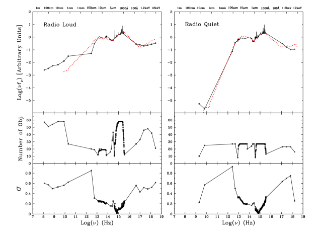
Figure 6: Top: Median SEDs for radio-loud and radio-quiet samples. Overploted are the mean SEDs (dotted line) of Elvis et al. (1994), normalized at about 4000 Å. Middle: Number of objects used to construct the SEDs in each wavelength bin marked with a small square. There are no data outside the bins. Bottom: Standard deviation around the mean in each wavelength bin. The data of the median SEDs are available in the online version of the Journal.

After having defined the bins for a sample of interest, we rebin the data to obtain one single value for each bin. This is mostly necessary for spectroscopic data, and this is done for each object separately so that all objects with available data will have equal weights in building the composite SED. Two RQ objects have upper limits in the highest radio frequency bin and six objects each for RL and RQ samples have upper limits in the MIPS 160µm band. They are included in the median combining process but none of the upper limits has a flux higher than the median value in the corresponding bin, therefore their uncertainty does not affect the composite SED. This median combining is very effective in rejecting outliers and preventing any extreme objects from dominating the final SEDs. We therefore also refer to our composite SEDs as median SEDs. Finally, if one bin has less than 8 points (i.e., objects), we exclude this bin from the median SED. Figure 6 shows our median SEDs for RL and RQ samples.

5.3 Discussion

We try to keep all the original data in building the SEDs of individual objects. The only change is the re-sampling of the UV-optical spectra to 10 Å resolution by rebinning. Although we lose some useful information (e.g. resolving narrow emission lines), this does not affect the SED work at all.

In constructing the composite SEDs, we applied rebinning again mostly for spectroscopic data. We did not apply any smoothing or interpolation in regions with real data, which could introduce systematic biases. The features in our median SEDs are real.

At the edges of some wavebands, the number of objects with data drops sharply (Fig. 6, middle), and our method of using median to build the composite SEDs can help to some extent in the small number statistics. We also visually check to ensure that the SEDs are reasonably smooth in those regions.

5.3.1 RL vs. RQ

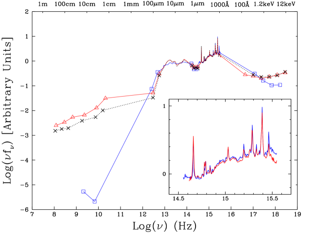
Figure 7: Median SEDs for the entire radio-loud sample (open triangle, red) and and radio-quiet sample (open square, blue). Also shown is the median SED for only the low-redshift radio-loud objects (cross, dotted-line) for comparison (§5.3.1). The inset shows only the UV-optical region.

Figure 7 overplots our median SEDs of RL and RQ samples, normalized at 4215 Å during the construction. The SEDs from FIR to UV are very similar for RL and RQ, especially in the UV-optical region. This is only true for the UV-optical continuum, because emission lines, such as Fe ii and [O iii], are known to strongly correlate with radio loudness in the Eigenvector I relationship (Boroson & Green, 1992). We will investigate the relationships between SEDs and emission line properties in a future paper.

The biggest difference between RL and RQ median SEDs is in the radio, where luminosity could differ by 3 orders of magnitude. There is also an obvious difference in the X-ray, where the RL objects are more X-ray luminous. This correlation between radio and X-ray luminosity has been reported in previous studies (e.g., Brinkmann et al., 2000; Polletta et al., 2007).

During the construction of the median SEDs, we have also defined 6 bins in the radio for the RQ sample (Table 10), however there are not enough objects ($\geq 8$) in 4 of the bins. Therefore, there are only two points good enough to be included in the final radio SED of RQ sample. Given the big difference in the number of objects involved in these two bins (Fig. 6), the apparent steep RQ spectral index, if defined using the two points, may not be reliable.

Our RL sample has more objects with higher redshifts than the RQ sample (Fig. 1). We therefore build another median SED of RL objects only with redshift less than 0.5 (21 objects), similar to those in the RQ sample. Comparing this and the SED of the entire RL sample (Fig. 7), we find that the only notable difference is in the radio where the low-z subsample shows a less luminous radio SED, but radio spectral index seems similar. The difference is probably real because of sample properties — high-z RL objects are more luminous in radio, but the differences between the RL and RQ samples are still much more prominent.

5.3.2 Comparison with E94 Mean SEDs

Elvis et al. (1994) use 47 objects to build the mean SEDs (MSED94) for RL and RQ objects. There are 11 objects in common with our sample, including 6 RL and 5 RQ objects. We compare our median SEDs of RL and RQ quasars (Fig. 6) with MSED94. The overall shape of the SEDs over the entire available frequency range is similar, but there are more detailed features in our new SEDs.

We specifically keep all the emission features in the UV-optical region because they are real spectral features and our data quality allows us to keep them. The underlying continuum shapes in this region look similar to those of MSED94. We note that our UV-optical SEDs extend to shorter wavelength beyond 1000 Å, and start to turn over, indicating the peak of the “big blue bump” (e.g., Zheng et al., 1998; Shang et al., 2005). This is especially obvious in our RL median SED where we have more higher redshift objects.

In the MIR, the broad silicate emission features around 10 and 18µm are prominent in the SEDs. These could not otherwise be reproduced without the unprecedented spectral data from Spitzer IRS. To the shorter wavelength of these features, a well-defined power-law rises up to about 4µm, the IRS detecting limit for our sample in the rest-frame. However, the well-known inflection around 1µm is also well defined by the red optical spectroscopy and NIR 2MASS photometry. It is therefore very clear that somewhere between 1 and 4µm, there is an infrared bump, which is further supported by the fact that the NIR K-band data point starts to rise toward MIR in both RL and RQ SEDs. Other studies have suggested that there is a 3µm bump, resulting from the hottest dust in AGNs (Netzer et al., 2007; Hiner et al., 2009).

Although MSED94 have a lot of upper limits in the FIR from IRAS while we use the latest Spitzer MIPS data, the SEDs agree surprisingly well for RQ sample in the FIR and extending to the radio.

For the RL sample, it is expected that our Spitzer data define a better FIR SED, which falls more steeply toward longer wavelengths. Our radio SED is more luminous than that of MSED94, simply because there are more radio-luminous objects in our sample.

5.3.3 Comparison with Quasar SEDs of Richards et al. (2006)

We compare our SEDs with those of Richards et al. (2006, hereafter R06) in Figure 8. R06 has provided the broadest frequency coverage, from Far-IR to X-ray, in recent SED studies, and their sample of 259 SDSS quasars extends to higher redshift and higher luminosity than ours. They constructed the SEDs using photometry points, including 5 SDSS magnitudes and 4 Spitzer InfraRed Array Camera (IRAC) flux densities, supplemented by available GALEX $f$ and $n$ bands, $J$, $H$, and $K$, the ISO 15 µm band, and the Spitzer MIPS 24 and 70 µm bands. When objects do not have measurements in the supplemental bands, they used Elvis et al. (1994) SEDs and their “gap repair” technique to estimate the missing values. Their X-ray fluxes were obtained from ROSAT detections. When no detection is available, they estimated the X-ray flux using the 2500 Å flux and the tight $L_{UV}(2500\mbox{\AA})$-$L_{X}$ relationship (Strateva et al., 2005). They have only 8 radio-loud quasars, so the final SEDs are essentially for radio-quiet quasars. Therefore, we only compare our radio-quiet SED with theirs, but plot both of our RL and RQ SEDs in Figure 8 for completeness. We further choose to compare only with their two SEDs constructed with optically red and blue halves of their sample, and their mean SED would lie between the two.

Our SEDs show relatively much higher X-ray emission, indicating that our sample (and that of Elvis et al. (1994)) is not representative of the SDSS quasars in this region and probably does not follow the $L_{UV}(2500\mbox{\AA})$-$L_{X}$ relationship found in SDSS quasars (Strateva et al., 2005). In the Far-IR to near-IR region, the overall shape and trend seem to match very well, but ours have more detailed features.

Although the SEDs are normalized at 4200 Å (Fig. 8), their shapes also match well over most of the UV-optical region. Only at the two ends, our SED show optical redder and UV brighter. This implies the different sample properties, because our objects are mostly UV-bright quasars and are probably redder in the $i$ band compared with R06 sample. Many objects in the R06 sample have much higher redshifts and luminosity than ours, but we do not have enough information to address any possible evolution or luminosity-dependent effects in quasar SEDs by comparing them.

5.3.4 Comparison with Other Quasar Composites

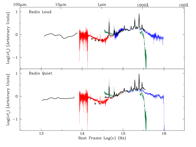
Figure 9: Median SEDs from FUV to MIR for our sample (black) compared with other quasar composite spectra, including the HST ultraviolet composites (blue, Telfer et al., 2002), the SDSS composite (green, Vanden Berk et al., 2001), and an NIR composite of 27 low-redshift SDSS quasars (red, Glikman et al., 2006). The SDSS and NIR composites do not distinguish radio-loud or radio-quiet objects. All composites are normalized at 4200 Å.

Figure 9 shows the comparison between our SEDs from Far-UV to Mid-IR and other quasar composite spectra, including the HST ultraviolet composites (Telfer et al., 2002), the composite from Sloan Digital Sky Survey (SDSS, Vanden Berk et al., 2001), and a Near-IR composite of 27 SDSS quasars (Glikman et al., 2006).

The HST composites extend beyond the FUV part of our SEDs to the extreme-UV (EUV), revealing the EUV peak more clearly. In the overlapping region, our SEDs are in good agreement with the HST composites although the radio-quiet HST composite drops a little steeper at higher frequency. The SDSS composite includes both radio-loud and radio quiet objects and is consistent with our SEDs between about 1200 and 4500 Å. The increased flux at the red part of the SDSS composite is partly due to host galaxy contamination at low redshift, while the blue part beyond ${\rm Ly}{\alpha}$ should be ignored because of ${\rm Ly}{\alpha}$ forest contamination. The NIR composites of radio-loud and radio-quiet samples show little difference in Glikman et al. (2006). We use the composite of their entire sample and its optical part matches our SEDs well. Its NIR region shows the 1µm inflection as expected, and the overall shape connects our MIR and optical SEDs surprisingly well. Although our NIR points are located a little lower than the composite, the continuum trends are consistent.

5.4 Uncertainty and Caveats

As in all previous quasar SED studies , the dispersion of the mean or composite SEDs is large. The dispersion of our median SEDs can be evaluated in Fig. 6, where population standard deviations of all rebinned points in each bin are plotted at the bottom. Because we normalized the individual SEDs at 4215 Å, the dispersion is minimized in the optical and increases toward both low and high frequencies to about 0.6 (dex) in radio and X-ray. Even in the NIR to UV region, the standard deviation increases rapidly away from the normalization wavelength.

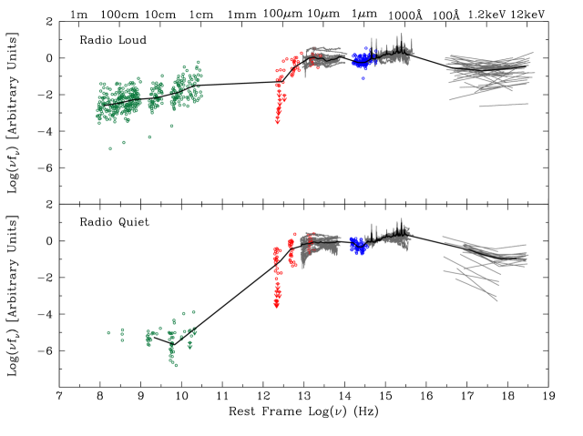
Figure 10: Dispersion of the median SEDs. All SEDs of individual objects, normalized at 4215 Å, are plotted together, showing large dispersions about the median SEDs (black thick line). Open circles are for radio (green), FIR (red), and NIR (blue) data. Spectroscopic data are shown in grey for MIR, UV/optical, and X-ray.

We also show the dispersion in Figure 10, where we plot all data from normalized SEDs of individual objects and the median SEDs built from them. The actual difference between the individual SEDs can be more than 2 orders of magnitude. Even in the NIR to UV, the difference is still more than one order of magnitude. These all indicate the large variation of quasar SEDs.

We note a caveat that the NIR host galaxy corrections may have a large uncertainty (§4.1, Table The Next Generation Atlas of Quasar Spectral Energy Distributions from Radio to X-rays), because the H-band host galaxy measurements with ground-based infrared data may be somewhat inherently uncertain. The host galaxy fractions from HST observations (McLeod & McLeod, 2001, and our own observations)are systematically smaller than those from ground-based observations (McLeod & Rieke, 1994a, b, and our IRTF data). Two objects have both ground-based and HST H-band observations and show revised lower host galaxy fractions from HST data (Table The Next Generation Atlas of Quasar Spectral Energy Distributions from Radio to X-rays), with PG 1322+659 from 43% to 22%, and PG 1427+480 from 45% to 26%, respectively. In addition, although the same technique was used in estimating the host galaxy fraction with all ground-based data, host galaxy fractions from McLeod & Rieke (1994a) and our IRTF data seem to be systematically higher than McLeod & Rieke (1994b) by about 20%. Some SEDs show discrepancy between NIR broad-band points and optical spectra (Fig. 4), indicating possible over-subtraction of host galaxy contributions. Readers should be aware of this issue when using data of this region for their own applications.

Our sample is heterogeneous, and there is the possibility that the sample may be biased. Jester et al. (2005) pointed out that BQS quasars are representative of bright blue quasars, but not representative of bright red quasars. Since our sample involves many PG quasars, it is possible that we might be missing some red quasars, and therefore the SEDs are not truly representative of $all$ UV-bright quasars. If this is true, it will affect the spectral index in the optical region. This does not seem to be a serious problem, however, because our SEDs do not show a drop off in the red part of the optical region when compared with the SEDs of R06 (Fig. 8). Moreover, even for the distinguished blue and red quasars in R06, except for the different spectral indices in the optical, their mean SEDs are very similar (see Fig. 8, or their Fig. 11), the largest difference in $log(\nu f_{\nu})$ is about 0.1 dex, significantly smaller than the dispersion of either R06 or our composite SEDs. Therefore, the large variation of individual quasar SEDs is still the dominant factor for the uncertainty of the composite SEDs.

6 SUMMARY AND FUTURE WORK

We have compiled SEDs for 85 quasars using high-quality multi-wavelength data from radio to X-ray energies. The data were obtained from the next generation space telescopes and ground-based telescopes. Using these data, we have constructed composite (median) SEDs for radio loud and radio quiet quasars. This work is an update on the mean SEDs built by Elvis et al. (1994) with about twice as many objects. On our website and the online version of the Journal, we make the electronic version of the median SEDs available for public use. We caution again that, because of the large variation in quasar SEDs, any composite SEDs should be used with care. Our composite SEDs are representative only for UV-optical bright quasars. The RQ median SED is constructed from low-redshift ($z<0.5$) objects, while the RL median SED comes from objects of redshift up to 1.4.

We also plan to investigate the multi-wavelength data of individual objects. We have measured all the spectral parameters of the entire sample and the work will be presented in a separate paper. We will be able to obtain the bolometric luminosities from real data and investigate the bolometric corrections associated with spectral properties, such as continua or emission features. We have also planned to investigate how the quasar SED varies with different physical parameters such as black hole mass and Eddington ratio. The multi-wavelength data will help us to better understand the quasars. A series of papers based on this data set are forthcoming.

Figure 1: Distributions of sample properties for radio-loud and radio-quiet sub-samples. Shaded bins are for radio-loud objects.

Figure 2: Examples of our collected data for two objects. Also marked are the wavebands and some instruments used to obtain the data.

Figure 3: Available Mid-Infrared spectra from Spitzer IRS for our sample. The bumps around 10 and 18 µm are silicate features.

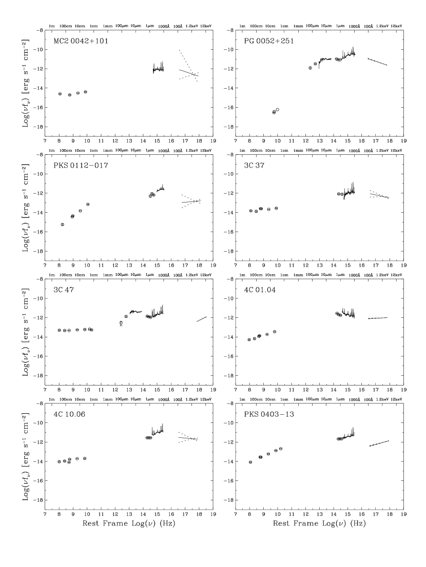
Figure 4: SEDs of the quasar sample, ordered by RA to match Table The Next Generation Atlas of Quasar Spectral Energy Distributions from Radio to X-rays. The flux ($\nu f_{\nu}$) is in observed-frame. Figures 4.1-4.11 are available in the online version of the Journal.

Figure 5: Example of defining bins in constructing composite SEDs for the RL sample. Open triangles are all data points from all RL objects. Vertical dotted-lines define the bins, each of which contributes one point in the final composite SED. Note the two small gaps with no data point between Log($\nu$) of 9 and 10. Shown on the right are the 2 FIR bins and MIR spectra where the bin size is much smaller.

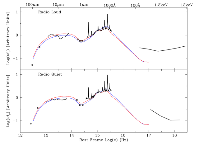
Figure 8: Median SEDs for our sample (black) compared with the SEDs of Richards et al. (2006) which are essentially for the radio-quiet quasars since there are only 8 radio-loud objects involved. The red and blue lines are for the optically red and blue halves of the population, respectively. The SEDs are normalized at 4200 Å.

Table 1: SED Sample

ID	Name	Other Name	RA(J2000)	DEC(J2000)	$z$	E(B$-$V)	R	$\lambda L_{\lambda}(3000\mbox{\AA})$	SampleID
1	MC2 0042+101		00:44:58.72	$+$10:26:53.7	0.5870	0.068	840string	46.22	RLQ
2	PG 0052+251		00:54:52.10	$+$25:25:38.0	0.1544	0.047	0.34	46.30	FUSE
3	PKS 0112$-$017	UM 310	01:15:17.10	$-$01:27:04.6	1.3743	0.062	2819string	45.92	RLQ
4	3C 37		01:18:18.49	$+$02:58:06.0	0.6661	0.039	5550string	45.64	RLQ
5	3C 47		01:36:24.40	$+$20:57:27.0	0.4250	0.061	6570string	44.94	RLQ
6	4C 01.04	PHL 1093	01:39:57.25	$+$01:31:46.2	0.2634	0.029	2556string	45.93	RLQ
7	4C 10.06	PKS 0214+10	02:17:07.66	$+$11:04:10.1	0.4075	0.109	472string	45.54	RLQ
8	PKS 0403$-$13		04:05:34.00	$-$13:08:13.7	0.5700	0.058	5413string	46.21	RLQ
9	3C 110	PKS 0414$-$06	04:17:16.70	$-$05:53:45.0	0.7749	0.043	477string	44.85	RLQ
10	3C 175	PKS 0710+11	07:13:02.40	$+$11:46:14.7	0.7693	0.147	978string	45.52	RLQ
11	3C 186		07:44:17.45	$+$37:53:17.1	1.0630	0.050	2131string	45.86	RLQ
12	B2 0742+31		07:45:41.67	$+$31:42:56.6	0.4616	0.068	591string	45.86	RLQ
13	IRAS F07546+3928	FBQS J075800.0+392029	07:58:00.05	$+$39:20:29.1	0.0953	0.066	0.25	45.23	FUSE
14	3C 207		08:40:47.59	$+$13:12:23.6	0.6797	0.093	4238string	46.32	RLQ
15	PG 0844+349	TON 951	08:47:42.40	$+$34:45:04.0	0.0643	0.037	0.07	45.06	FUSE
16	PKS 0859$-$14		09:02:16.83	$-$14:15:30.9	1.3320	0.062	2683string	44.63	RLQ
17	3C 215		09:06:31.90	$+$16:46:11.4	0.4108	0.040	2328string	46.54	RLQ
18	4C 39.25	B2 0923+39	09:27:03.01	$+$39:02:20.9	0.6946	0.014	4512string	45.70	RLQ
19	4C 40.24		09:48:55.34	$+$40:39:44.6	1.2520	0.014	8699string	46.41	RLQ
20	PG 0947+396		09:50:48.39	$+$39:26:50.5	0.2057	0.019	0.31	45.30	FUSE,PGX
21	PG 0953+414		09:56:52.40	$+$41:15:22.0	0.2338	0.013	0.61	46.16	FUSE,PGX
22	4C 55.17		09:57:38.18	$+$55:22:57.8	0.8990	0.009	5525string	46.11	RLQ
23	3C 232		09:58:20.95	$+$32:24:02.2	0.5297	0.015	736string	45.65	RLQ
24	PG 1001+054		10:04:20.09	$+$05:13:00.5	0.1603	0.016	1.12	45.43	PGX
25	4C 22.26	PKS 1002+22	10:04:45.74	$+$22:25:19.4	0.9760	0.039	1817string	45.99	RLQ
26	4C 41.21		10:10:27.52	$+$41:32:38.9	0.6124	0.015	820string	45.31	RLQ
27	4C 20.24	PKS 1055+20	10:58:17.90	$+$19:51:50.9	1.1135	0.025	4152string	46.12	RLQ
28	PG 1100+772	3C 249.1	11:04:13.69	$+$76:58:58.0	0.3114	0.034	444string	45.83	FUSE,RLQ
29	PG 1103$-$006	PKS 1103$-$006	11:06:31.77	$-$00:52:52.5	0.4234	0.044	868string	45.95	RLQ
30	3C 254		11:14:38.48	$+$40:37:20.3	0.7363	0.015	5139string	45.08	RLQ
31	PG 1114+445		11:17:06.40	$+$44:13:33.0	0.1440	0.016	0.11	45.76	PGX
32	PG 1115+407		11:18:30.20	$+$40:25:53.0	0.1541	0.016	0.33	46.53	PGX
33	PG 1116+215	TON 1388	11:19:08.60	$+$21:19:18.0	0.1759	0.023	0.73	46.01	PGX
34	4C 12.40	MRC 1118+128	11:21:29.79	$+$12:36:17.4	0.6836	0.029	1071string	45.81	RLQ
35	PKS 1127$-$14		11:30:07.05	$-$14:49:27.4	1.1870	0.037	7581string	45.95	RLQ
36	3C 263		11:39:57.04	$+$65:47:49.4	0.6464	0.011	997string	45.91	RLQ
37	MC2 1146+111		11:48:47.89	$+$10:54:59.4	0.8614	0.043	358string	45.42	RLQ
38	4C 49.22	LB 02136	11:53:24.46	$+$49:31:08.8	0.3333	0.021	2268string	46.30	RLQ
39	TEX 1156+213		11:59:26.20	$+$21:06:55.0	0.3480	0.027	238string	44.99	RLQ
40	PG 1202+281	GQ COM	12:04:42.10	$+$27:54:11.0	0.1651	0.021	1.09	45.03	PGX
41	4C 64.15		12:17:41.85	$+$64:07:07.8	1.3000	0.019	2365string	45.67	RLQ
42	PG 1216+069		12:19:20.88	$+$06:38:38.4	0.3319	0.022	4.64	43.68	PGX
43	PG 1226+023	3C 273	12:29:06.70	$+$02:03:08.6	0.1576	0.021	1667string	44.46	FUSE,PGX,RLQ
44	4C 30.25	B2 1248+30	12:50:25.55	$+$30:16:39.3	1.0610	0.016	831string	45.98	RLQ
45	3C 277.1		12:52:26.35	$+$56:34:19.7	0.3199	0.010	3354string	45.13	RLQ
46	PG 1259+593		13:01:12.90	$+$59:02:06.4	0.4769	0.008	0.02	44.62	FUSE
47	3C 281		13:07:54.00	$+$06:42:14.3	0.6017	0.039	1683string	45.06	RLQ
48	PG 1309+355	TON 1565	13:12:17.77	$+$35:15:21.2	0.1823	0.012	23.81	45.70	PGX
49	PG 1322+659		13:23:49.54	$+$65:41:48.0	0.1684	0.019	0.16	44.61	FUSE,PGX
50	3C 288.1		13:42:13.18	$+$60:21:42.9	0.9631	0.018	2660string	45.67	RLQ
51	PG 1351+640	IRAS F13517+6400	13:53:15.81	$+$63:45:45.4	0.0882	0.020	1.24	45.57	FUSE
52	B2 1351+31		13:54:05.35	$+$31:39:01.9	1.3260	0.017	888string	44.94	RLQ
53	PG 1352+183		13:54:35.60	$+$18:05:17.2	0.1510	0.019	0.24	44.89	PGX
54	4C 19.44		13:57:04.43	$+$19:19:07.4	0.7192	0.060	2632string	45.42	RLQ
55	4C 58.29		13:58:17.63	$+$57:52:04.9	1.3740	0.010	453string	44.70	RLQ
56	PG 1402+261	TON 182	14:05:16.19	$+$25:55:34.9	0.1650	0.016	0.30	45.50	PGX
57	PG 1411+442		14:13:48.30	$+$44:00:14.0	0.0895	0.008	0.14	46.26	PGX
58	PG 1415+451		14:17:00.80	$+$44:56:06.0	0.1143	0.009	0.27	46.07	PGX
59	PG 1425+267	TON 202	14:27:35.54	$+$26:32:13.6	0.3637	0.019	206string	45.19	PGX
60	PG 1427+480		14:29:43.00	$+$47:47:26.0	0.2203	0.017	0.03	44.92	PGX
61	PG 1440+356	MRK 478	14:42:07.46	$+$35:26:22.9	0.0773	0.014	0.18	44.79	PGX
62	PG 1444+407		14:46:45.90	$+$40:35:05.0	0.2673	0.014	0.10	44.80	PGX
63	PG 1512+370	4C 37.43	15:14:43.04	$+$36:50:50.4	0.3700	0.022	717string	45.20	PGX
64	PG 1534+580	MRK 290	15:35:52.36	$+$57:54:09.2	0.0303	0.015	1.37	44.89	FUSE
65	PG 1543+489	IRAS F15439+4855	15:45:30.20	$+$48:46:09.0	0.4000	0.018	1.36	44.59	PGX
66	PG 1545+210	3C 323.1	15:47:43.54	$+$20:52:16.7	0.2642	0.042	1000string	45.52	RLQ
67	B2 1555+33		15:57:29.94	$+$33:04:47.0	0.9420	0.038	975string	45.02	RLQ
68	B2 1611+34	DA 406	16:13:41.06	$+$34:12:47.9	1.3945	0.018	5825string	44.83	RLQ
69	3C 334		16:20:21.92	$+$17:36:24.0	0.5553	0.041	1294string	45.51	RLQ
70	PG 1626+554		16:27:56.00	$+$55:22:31.0	0.1317	0.006	0.10	45.53	PGX
71	OS 562		16:38:13.45	$+$57:20:24.0	0.7506	0.013	2248string	43.51	RLQ
72	PKS 1656+053		16:58:33.45	$+$05:15:16.4	0.8890	0.159	1268string	45.65	RLQ
73	PG 1704+608	3C 351	17:04:41.37	$+$60:44:30.5	0.3730	0.023	666string	45.28	FUSE,RLQ
74	MRK 506		17:22:39.90	$+$30:52:53.0	0.0428	0.031	3.11	44.90	FUSE
75	4C 34.47	B2 1721+34	17:23:20.80	$+$34:17:57.9	0.2055	0.037	419string	45.81	FUSE
76	4C 73.18		19:27:48.49	$+$73:58:01.6	0.3027	0.133	1587string	44.82	RLQ
77	MRK 509	IRAS F20414$-$1054	20:44:09.74	$-$10:43:24.5	0.0345	0.057	0.58	45.74	FUSE
78	4C 06.69	PKS 2145+06	21:48:05.46	$+$06:57:38.6	1.0002	0.080	2102string	45.03	RLQ
79	4C 31.63	B2 2201+31A	22:03:14.97	$+$31:45:38.3	0.2952	0.124	853string	46.24	RLQ
80	PG 2214+139	MRK 304	22:17:12.26	$+$14:14:21.1	0.0657	0.073	0.04	45.64	FUSE
81	PKS 2216$-$03	4C $-$03.79	22:18:52.04	$-$03:35:36.9	0.8993	0.095	1708string	46.54	RLQ
82	3C 446		22:25:47.26	$-$04:57:01.4	1.4040	0.075	21719string	46.35	RLQ
83	4C 11.69	PKS 2230+11	22:32:36.41	$+$11:43:50.9	1.0370	0.072	5992string	46.31	RLQ
84	PG 2251+113	PKS 2251+11	22:54:10.40	$+$11:36:38.3	0.3253	0.086	291string	46.36	RLQ
85	PG 2349$-$014	PKS 2349$-$10	23:51:56.13	$-$01:09:13.3	0.1740	0.027	556string	45.23	FUSE

Table 2: Radio Surveys

Frequency		Number of	Resolution
(MHz)	Surveys	Objects Included	(″)	References
74	VLSS	57	45	1
151	7C	30	70	2
178	4C	44	1380-1860	3
325	WENSS	29	54	4
365	TEXAS	55	22.1	5
408	MRC	23	157	6
1400	NVSS/FIRST	64/3	45/5	7
1420	Ulvestad.2005	2	$<0.01$	8
1490	Barvainis.1996	4	$<40$	9
2270	Ulvestad.2005	2	$<0.01$	8
4800	Leipski.2006	3	$<1.7$	10
4850	GB6	50	210	11
4850	PMN	8	252	12
4890	Barvainis.1996	6	$<40$	9
4990	Ulvestad.2005	2	$<0.01$	8
5000	Kellermann.1989	21	0.5	13
5000	Gear.1994	2	714	14
8000	Gear.1994	3	444	14
8480	Barvainis.1996	3	$<40$	9
8600	Barvainis.2005	1	$\sim 1.3$	15
10700	Kellermann.1973	24	171	16
14000	Gear1994	3	252	14
14900	Genzel.1976	12	59	17
14900	Barvainis.1996	6	$<40$	9
15200	Bolton.2004	1	$<252$	18

Note. — Radio surveys and references used to collect SED data.

References. — (1) The VLA Low-Frequency Sky Survey (Cohen et al., 2007); (2) 7C 151-MHz Survey (Hales et al., 2007); (3) 4C Survey (Pilkington & Scott, 1965; Gower et al., 1967); (4) The Westerbork Northern Sky Survey (Rengelink et al., 1997; Leiden, 1998); (5) The Texas Survey of Radio Sources (Douglas et al., 1996); (6) The Molonglo Reference Catalogue of Radio Sources (Large et al., 1981, 1991); (7) The NRAO VLA Sky Survey (Condon et al., 1998); Faint Images of the Radio Sky at Twenty-Centimeters (Becker et al., 1995); (8) Ulvestad et al. (2005); (9) Barvainis et al. (1996); (10) Leipski et al. (2006); (11) GB6 (12) The Parkes-MIT-NRAO (Griffith et al., 1995); (13) Kellermann et al. (1989); (14) Gear et al. (1994); (15) Barvainis et al. (2005); (16) Kellermann & Pauliny-Toth (1973); (17) Genzel et al. (1976); (18) Bolton et al. (2004).

Table 3: Radio Fluxes

ID	Object	$\nu$(MHz)	$f_{\nu}$(mJy)	$\Delta f_{\nu}$ (mJy)	Reference
1	MC2 0042+101	74	3380	390	VLSS
		365	540	47	TEXAS
		1400	218.8	7.0	NVSS
		4850	83	8.1	GB6
2	PG 0052+251	4800	0.61	0.03	Leipski.2006
		5000	0.74		Kellermann.1989
		8600	0.7		Barvainis.2005
3	PKS 0112$-$017	74	780	120	VLSS
		365	974	25	TEXAS
		408	1110	70	MRC
		1400	1076.2	32.3	NVSS
		4850	1437	75	PMN

Note. — Table 3 is published in its entirety in the electronic edition of ApJS. A portion is shown here for guidance regarding its form and content.

Table 4: Spitzer MIPS FIR Fluxes

		Flux (mJy)
ID	Object	24µm	70µm	160µm
2	PG 0052+251	$70.\pm 3.4$	$76.1\pm 9.1$	$65.1\pm 14.$
5	3C 47	$33.5\pm 2.35$	$31.\pm 5.14$	$15.2\pm 7.58$
10	3C 175	$12.3\pm 1.43$	$25.3\pm 5.06$	$<2.5$
11	3C 186	$6.79\pm 1.06$	$\cdots$	$\cdots$
13	IRAS F07546+3928	$220.\pm 6.03$	$154.\pm 11.5$	$<1.08$
14	3C 207	$11.9\pm 1.4$	$23.7\pm 4.56$	$57.8\pm 13.1$
15	PG 0844+349	$92.4\pm 3.91$	$63.2\pm 7.93$	$107.\pm 18.1$
20	PG 0947+396	$49.8\pm 2.87$	$117.\pm 10.2$	$111.\pm 18.3$
21	PG 0953+414	$42.\pm 2.64$	$18.\pm 5.81$	$16.6\pm 7.12$
24	PG 1001+054	$35.9\pm 2.44$	$36.4\pm 6.09$	$<0.128$
28	PG 1100+772	$46.\pm 2.76$	$63.9\pm 7.07$	$16.8\pm 8.21$
29	PG 1103$-$006	$32.5\pm 2.32$	$21.9\pm 5.52$	$17.6\pm 7.58$
30	3C 254	$12.2\pm 1.42$	$11.7\pm 3.18$	$11.6\pm 6.11$
31	PG 1114+445	$133.\pm 4.69$	$50.3\pm 6.85$	$<1.15$
32	PG 1115+407	$44.\pm 2.7$	$175.\pm 11.9$	$143.\pm 20.6$
33	PG 1116+215	$102.\pm 4.11$	$63.1\pm 8.43$	$30.5\pm 9.69$
36	3C 263	$28.6\pm 2.18$	$50.8\pm 7.02$	$18.1\pm 7.44$
40	PG 1202+281	$81.2\pm 3.67$	$112.\pm 10.1$	$32.8\pm 10.2$
42	PG 1216+069	$24.2\pm 2.01$	$15.4\pm 4.66$	$<0.845$
43	PG 1226+023	$511.\pm 9.2$	$488.\pm 20.2$	$299.\pm 29.8$
45	3C 277.1	$20.5\pm 1.85$	$21.4\pm 4.12$	$<1.29$
46	PG 1259+593	$21.2\pm 1.87$	$10.7\pm 3.7$	$9.03\pm 5.51$
48	PG 1309+355	$104.\pm 4.15$	$85.8\pm 8.86$	$45.9\pm 11.7$
49	PG 1322+659	$43.3\pm 2.68$	$113.\pm 10.$	$92.3\pm 16.7$
50	3C 288.1	$8.32\pm 1.17$	$\cdots$	$\cdots$
51	PG 1351+640	$423.\pm 8.36$	$567.\pm 21.7$	$187.\pm 23.6$
53	PG 1352+183	$31.6\pm 2.29$	$10.1\pm 4.07$	$<0.164$
56	PG 1402+261	$100.\pm 4.08$	$263.\pm 14.8$	$86.6\pm 16.2$
57	PG 1411+442	$122.\pm 4.48$	$101.\pm 9.04$	$70.4\pm 14.5$
58	PG 1415+451	$59.3\pm 3.13$	$96.6\pm 8.87$	$54.4\pm 12.7$
59	PG 1425+267	$42.7\pm 2.66$	$75.8\pm 8.25$	$14.9\pm 6.86$
60	PG 1427+480	$41.9\pm 2.63$	$91.7\pm 9.4$	$<1.06$
61	PG 1440+356	$177.\pm 5.42$	$738.\pm 24.5$	$438.\pm 36.$
62	PG 1444+407	$60.\pm 3.15$	$75.6\pm 8.53$	$37.\pm 10.6$
63	PG 1512+370	$31.4\pm 2.28$	$37.3\pm 5.77$	$<0.999$
64	PG 1534+580	$173.\pm 5.34$	$172.\pm 11.6$	$60.4\pm 13.4$
65	PG 1543+489	$101.\pm 4.09$	$285.\pm 15.$	$82.8\pm 15.7$
66	PG 1545+210	$33.8\pm 2.37$	$19.4\pm 3.96$	$<0.528$
67	B2 1555+33	$3.44\pm 0.757$	$\cdots$	$\cdots$
69	3C 334	$35.2\pm 2.41$	$86.9\pm 8.58$	$18.4\pm 7.39$
70	PG 1626+554	$16.5\pm 1.65$	$16.3\pm 4.38$	$4.83\pm 3.8$
73	PG 1704+608	$105.\pm 4.16$	$188.\pm 12.2$	$41.6\pm 11.3$
74	MRK 506	$82.6\pm 3.69$	$196.\pm 12.7$	$292.\pm 29.4$
75	4C 34.47	$55.2\pm 3.02$	$27.1\pm 4.73$	$<0.326$
77	MRK 509	$602.\pm 9.97$	$1440.\pm 34.4$	$689.\pm 45.2$
79	4C 31.63	$70.4\pm 3.41$	$79.7\pm 8.24$	$33.7\pm 10.$
80	PG 2214+139	$94.8\pm 3.96$	$79.6\pm 8.66$	$48.1\pm 12.$
83	4C 11.69	$33.4\pm 2.35$	$138.\pm 10.6$	$150.\pm 21.1$
84	PG 2251+113	$43.8\pm 2.69$	$59.7\pm 7.46$	$<1.21$
85	PG 2349$-$014	$72.\pm 3.45$	$155.\pm 11.8$	$88.2\pm 16.2$

Note. — The upper limits for 160 µm are 3$\sigma$ limits, where $\sigma$ is the standard deviation of the local sky background.

Table 5: Near-IR JHK Magnitudes from 2MASS

Note. — The 2MASS magnitudes are obtained from both profile fitting photometry and aperture photometry. Values without uncertainties reflect the fact that the original sources did not provide uncertainties.

Table 6: Total JHK Magnitudes and Observed Host Fraction

Note. — Total magnitude is adopted from 2MASS aperture magnitude in Table The Next Generation Atlas of Quasar Spectral Energy Distributions from Radio to X-rays.

Table 7: Host Corrected JHK Magnitude and Flux

Note. — For objects without H-band host fraction, we take 2MASS profile fitting magnitude as the AGN magnitude. Values without uncertainties reflect the fact that the original sources did not provide uncertainties.

Table 8: Far-UV FUSE Data

		Rest Wavelength (Å)		Flux
ID	Object	$\lambda$1	$\lambda$2	($10^{-14}$ erg s-1 cm-2 Å-1)
(1)	(2)	(3)	(4)	(5)
2	PG 0052+251	789	1028	1.67
13	IRAS F07546+3928	832	1083	0.72
15	PG 0844+349	856	1115	4.83
20	PG 0947+396	758	984	1.12
21	PG 0953+414	740	962	5.84
28	PG 1100+772	696	905	1.50
33	PG 1116+215	768	1010	6.58
36	3C 263	549	721	1.19
42	PG 1216+069	678	892	1.16
43	PG 1226+023	787	1025	27.36
46	PG 1259+593	618	803	1.90
49	PG 1322+659	781	1015	1.21
51	PG 1351+640	837	1090	1.91
56	PG 1402+261	776	1020	3.15
58	PG 1415+451	811	1066	1.27
61	PG 1440+356	839	1103	5.27
64	PG 1534+580	885	1151	3.29
70	PG 1626+554	798	1050	0.67
73	PG 1704+608	664	864	0.16
74	MRK 506	874	1138	1.74
75	4C 34.47	757	984	0.60
77	MRK 509	885	1145	11.01
80	PG 2214+139	855	1113	2.23
85	PG 2349$-$014	777	1011	1.84

Table 9: X-ray Spectral Parameters (Single or Broken Power-law)

Note. — E1, E2, and E3 are the observed-frame energies (in keV) at which the power-law models are fit. When broken power-law models are used, E2 and columns (8)-(9) are needed to present them. $f_{0}$ is flux density at 1 keV, in units of mJy ($10^{-26}$ erg s^-1 cm^-2 Hz^-1); $E$ in keV. Values without uncertainties reflect the fact that the original sources did not provide uncertainties.

References. — R,C,X indicate data sources, corresponding to ROSAT, Chandra, and XMM, respectively. Br97—Brinkmann et al. 1997; Yu98—Yuan et al. 1998; La97—Laor et al. 1997; Be06—Belsole et al. 2006; Ha96—Hardcastle et al. 2006; Sh05—Shi et al. 2005; Sa06—Sambruna et al. 2006; Ga03—Gambill et al. 2003; Ta07—Tavecchio et al. 2007; Si08—Siemiginowska et al. 2008; CSC—Chandra Source Catalog; Pi05—Piconcelli et al. 2005; Po04—Porquet et al. 2004; Fo06—Foschini et al. 2008

Table 10: Parameters of Defining Bins in Each Waveband

Wavelength	Radio-Loud					Radio-Quiet
Band	$\nu 1$	$\nu 2$	Bins	$\Delta\nu$		$\nu 1$	$\nu 2$	Bins	$\Delta\nu$
radio	7.90	9.02	3	0.373		7.90	9.02	3	0.373
radio	9.18	9.55	1	0.370		9.13	9.51	1	0.380
radio	9.71	10.52	2	0.405		9.67	10.31	2	0.320
FIR	12.33	12.89	2	0.280		12.28	12.81	2	0.265
MIR	13.06	13.90	30	0.028		12.91	13.83	30	0.031
NIR	14.20	14.54	4	0.085		14.15	14.49	3	0.113
UV/opt	14.61	15.55	200	0.005		14.55	15.55	200	0.005
X-ray	16.46	18.63	6	0.362		16.88	18.41	4	0.383

Note. — See §5.2 on how the bins are defined in constructing composite SEDs.

References

- Baldwin (1977) Baldwin, J. A. 1977, ApJ, 214, 679
- Barvainis et al. (2005) Barvainis, R., Lehár, J., Birkinshaw, M., Falcke, H., & Blundell, K. M. 2005, ApJ, 618, 108
- Barvainis et al. (1996) Barvainis, R., Lonsdale, C., & Antonucci, R. 1996, AJ, 111, 1431
- Becker et al. (1995) Becker, R. H., White, R. L., & Helfand, D. J. 1995, ApJ, 450, 559
- Bohlin (1996) Bohlin, R. C. 1996, AJ, 111, 1743
- Bohlin (2000) Bohlin, R. C. 2000, AJ, 120, 437
- Bolton et al. (2004) Bolton, R. C., et al. 2004, MNRAS, 354, 485
- Boroson & Green (1992) Boroson, T. A, & Green, R. F. 1992, ApJS, 80, 109 (BG92)
- Brinkmann, Yuan, & Siebert (1997) Brinkmann, W., Yuan, W., & Siebert, J. 1997, A&A, 319, 413
- Brinkmann et al. (2000) Brinkmann, W., Laurent-Muehleisen, S. A., Voges, W., Siebert, J., Becker, R. H., Brotherton, M. S., White, R. L., & Gregg, M. D. 2000, A&A, 356, 445
- Cardelli et al. (1989) Cardelli, J. A., Clayton, G. C., & Mathis, J. S., 1989, ApJ, 345, 245
- Cohen et al. (2007) Cohen, A. S., Lane, W. M., Cotton, W. D., Kassim, N. E., Lazio, T. J. W., Perley, R. A., Condon, J. J., & Erickson, W. C. 2007, AJ, 134, 1245
- Condon et al. (1998) Condon, J. J., Cotton, W. D., Greisen, E. W., Yin, Q. F., Perley, R. A., Taylor, G. B., & Broderick, J. J. 1998, AJ, 115, 1693
- Dale et al. (2007) Dale, D. A., et al. 2007, ApJ, 655, 863
- Dale et al. (2009) Dale, D. A., et al. 2009, ApJ, 693, 1821
- Diamond-Stanic et al. (2009) Diamond-Stanic, A. M., Rieke, G. H., & Rigby, J. R. 2009, ApJ, 698, 623
- Douglas et al. (1996) Douglas, J. N., Bash, F. N., Bozyan, F. A., Torrence, G. W., & Wolfe, C. 1996, AJ, 111, 1945
- Edelson & Malkan (1986) Edelson, R. A., & Malkan, M. A. 1986, ApJ, 308, 59
- Elvis et al. (1994) Elvis, M., Wilkes, B. J., McDowell, J. C., Green, R. F., Bechtold, J., Willner, S. P., Oey, M. S., Polomski, E., & Cutri, R. 1994, ApJS, 95, 1
- Evans et al. (2010) Evans, I. N., et al. 2010, ApJS, 189, 37
- Gear et al. (1994) Gear, W. K., et al. 1994, MNRAS, 267, 167
- Gallagher et al. (2007) Gallagher, S. C., Hines, D. C., Blaylock, M., Priddey, R. S., Brandt, W. N., & Egami, E. E. 2007, ApJ, 665, 157
- Genzel et al. (1976) Genzel, R., Pauliny-Toth, I. I. K., Preuss, E., & Witzel, A. 1976, AJ, 81, 1084
- Glikman et al. (2006) Glikman, E., Helfand, D. J., & White, R. L. 2006, ApJ, 640, 579
- Goulding & Alexander (2009) Goulding, A. D., & Alexander, D. M. 2009, MNRAS, 398, 1165
- Grupe et al. (2010) Grupe, D., Komossa, S., Leighly, K. M., & Page, K. L. 2010, ApJS, 187, 64
- Pilkington & Scott (1965) Pilkington, J. D. H., & Scott, P. F. 1965, MmRAS, 69, 183
- Gower et al. (1967) Gower, J. F. R., Scott, P. F., & Wills, D. 1967, MmRAS, 71, 49
- Griffith et al. (1995) Griffith, M. R., Wright, A. E., Burke, B. F., & Ekers, R. D. 1995, ApJS, 97, 347
- Hales et al. (2007) Hales, S. E. G., Riley, J. M., Waldram, E. M., Warner, P. J., & Baldwin, J. E. 2007, MNRAS, 382, 1639
- Hao et al. (2005) Hao, L., et al. 2005, ApJ, 625, L75
- Hiner et al. (2009) Hiner, K. D., Canalizo, G., Lacy, M., Sajina, A., Armus, L., Ridgway, S., & Storrie-Lombardi, L. 2009, ApJ, 706, 508
- Houck et al. (2004) Houck, J. R., et al. 2004, ApJS, 154, 18
- Jester et al. (2005) Jester, S., et al. 2005, AJ, 130, 873
- Kellermann & Pauliny-Toth (1973) Kellermann, K. I., & Pauliny-Toth, I. I. K. 1973, AJ, 78, 828
- Kellermann et al. (1989) Kellermann, K. I., Sramek, R., Schmidt, M., Shaffer, D. B., & Green, R. 1989, AJ, 98, 1195
- Kriss (1988) Kriss, G. A. 1988, ApJ, 324, 809
- Kriss (2000) Kriss, G. J. 2000, in ASP conf. Series 224, Probing the Physics of Active Galactic Nuclei, ed. B. M. Peterson, R. W. Pogge, & R. S. Polidan (San Francisco: ASP), 45
- Kuraszkiewicz et al. (2003) Kuraszkiewicz, J. K., et al. 2003, ApJ, 590, 128
- Kuraszkiewicz et al. (2009) Kuraszkiewicz, J., et al. 2009, ApJ, 692, 1143
- Large et al. (1981) Large, M. I., Mills, B. Y., Little, A. G., Crawford, D. F., & Sutton, J. M. 1981, MNRAS, 194, 693
- Large et al. (1991) Large, M. I., Cram, L. E., & Burgess, A. M. 1991, The Observatory, 111, 72
- Laor et al. (1994) Laor, A., Fiore, F., Elvis, M., Wilkes, B. J., & McDowell, J. C. 1994, ApJ, 435, 611 The soft x-ray properties of a complete sample of optically selected quasars. 1: First results
- Laor et al. (1997) Laor, A., Fiore, F., Elvis, M., Wilkes, B. J., & McDowell, J. C. 1997, ApJ, 477, 93
- Leiden (1998) de Bruyn, G., Miley, G., Rengelink, R., Tang, Y., Bremer, M., Rottgering, H., Raimond, R., Bremer, M., & Fullagar, D. 1998, The Westerbork Northern Sky Survey, http://cdsarc.u-strasbg.fr/viz-bin/Cat?VIII/62
- Leipski et al. (2006) Leipski, C., Falcke, H., Bennert, N., Huttemeister, S. 2006, A&A, 455, 161
- McLeod & Rieke (1994a) McLeod, K. K., & Rieke, G. H. 1994a, ApJ, 420, 58
- McLeod & Rieke (1994b) McLeod, K. K., & Rieke, G. H. 1994b, ApJ, 431, 137
- McLeod & Rieke (1995) McLeod, K. K., & Rieke, G. H. 1995, ApJ, 454, L77
- McLeod & McLeod (2001) McLeod, K. K., & McLeod, B. A. 2001, ApJ, 546, 782
- Moos et al. (2000) Moos, H. W., et al. 2000, ApJ, 538, L1
- Nemmen & Brotherton (2010) Nemmen, R. S., & Brotherton, M. S. 2010, MNRAS, 408, 1598
- Netzer et al. (1995) Netzer, H., Brotherton, M. S., Wills, B. J., Han, M., Wills, D., Baldwin, J. A., Ferland, G. J., & Browne, I. W. A. 1995, ApJ, 448, 27
- Netzer et al. (2007) Netzer, H., et al. 2007, ApJ, 666, 806
- Peng et al. (2002) Peng, C. Y., Ho, L. C., Impey, C. D., & Rix, H.-W. 2002, AJ, 124, 266
- Pereira-Santaella et al. (2010) Pereira-Santaella, M., Diamond-Stanic, A. M., Alonso-Herrero, A., & Rieke, G. H. 2010, ApJ, 725, 2270
- Polletta et al. (2000) Polletta, M., Courvoisier, T. J.-L., Hooper, E. J., & Wilkes, B. J. 2000, A&A, 362, 75
- Polletta et al. (2007) Polletta, M., et al. 2007, ApJ, 663, 81
- Rengelink et al. (1997) Rengelink, R. B., Tang, Y., de Bruyn, A. G., Miley, G. K., Bremer, M. N., Roettgering, H. J. A., & Bremer, M. A. R. 1997, A&AS, 124, 259
- Rieke et al. (2004) Rieke, G. H., et al. 2004, ApJS, 154, 25
- Risaliti & Elvis (2004) Risaliti, G., & Elvis, M. 2004, Supermassive Black Holes in the Distant Universe, 308, 187
- Richards et al. (2006) Richards, G. T., et al. 2006, ApJS, 166, 470
- Runnoe et al. (2011) Runnoe, J. et al. 2011, in preparation.
- Sanders et al. (1989) Sanders, D. B., Phinney, E. S., Neugebauer, G., Soifer, B. T., & Matthews, K. 1989, ApJ, 347, 29
- Schlegel, Finkbeiner, & Davis (1998) Schlegel, D. J., Finkbeiner, D. P., & Davis, M. 1998, ApJ, 500, 525
- Schmidt & Green (1983) Schmidt, M., & Green, R. F. 1983, ApJ, 269, 352
- Schweitzer et al. (2006) Schweitzer, M., et al. 2006, ApJ, 649, 79
- Shang et al. (2003) Shang, Z., Wills, B. J., Robinson, E. L., Wills, D., Laor, A., Xie, B., & Yuan, J. 2003, ApJ, 586, 52
- Shang et al. (2005) Shang, Z, Brotherton, M. S., Green, R. F., Kriss, G. A., Scott, J., Quijano, J. K., Blaes, O., Hubeny, I., Hutchings, J., Kaiser, M. E., Koratkar, A., Oegerle, W., Zheng, W. 2005, ApJ, 619, 41
- Shang et al. (2007) Shang, Z., Wills, B. J., Wills, D., & Brotherton, M. S. 2007, AJ, 134, 294
- Skrutskie et al. (2006) Skrutskie, M. F., et al. 2006, AJ, 131, 1163
- Strateva et al. (2005) Strateva, I. V., Brandt, W. N., Schneider, D. P., Vanden Berk, D. G., & Vignali, C. 2005, AJ, 130, 387
- Sun & Malkan (1989) Sun, W.-H., & Malkan, M. A. 1989, ApJ, 346, 68
- Telfer et al. (2002) Telfer, R. C., Zheng, W., Kriss, G. A., & Davidsen, A. F. 2002, ApJ, 565, 773
- Tommasin et al. (2010) Tommasin, S., Spinoglio, L., Malkan, M. A., & Fazio, G. 2010, ApJ, 709, 1257
- Ulvestad et al. (2005) Ulvestad, J. S., Antonucci, R. R. J., & Barvainis, R. 2005, ApJ, 621, 123
- Vanden Berk et al. (2001) Vanden Berk, D. et al. 2001, AJ, 122, 549
- Ward et al. (1987) Ward, M., Elvis, M., Fabbiano, G., Carleton, N. P., Willner, S. P., & Lawrence, A. 1987, ApJ, 315, 74
- Weedman et al. (2005) Weedman, D. W., et al. 2005, ApJ, 633, 706
- Werner et al. (2004) Werner, M. W., et al. 2004, ApJS, 154, 1
- Wills et al. (1995) Wills, B. J., et al. 1995, ApJ, 447, 139
- Wilkes et al. (1999) Wilkes, B. J., Kuraszkiewicz, J., Green, P. J., Mathur, S., & McDowell, J. C. 1999, ApJ, 513, 76
- Zheng et al. (1998) Zheng, W., Kriss, G. A., Telfer, R. C., Grimes, J. P., & Davidsen, A. F. 1998, ApJ, 492, 855
- Zheng et al. (2001) Zheng, W., et al. 2001, ApJ, 562, 152