Entanglement generation between unstable optically active qubits without photodetectors

Abstract

We propose a robust deterministic scheme to generate entanglement at high fidelity without the need of photodetectors even for quantum bits, qubits, with extremely poor optically active states. Our protocol employs stimulated Raman adiabatic passage for population transfer without actually exciting the system. Furthermore, it is found to be effective even if the environmental decoherence rate is of the same order of magnitude as the atom–photon coupling frequency. Our scheme holds potential to solve entanglement generation problems, e.g., in distributed quantum computing.

One of the key challenges for practical quantum computing is scalability. Recently, an approach referred to as distributed quantum information processing has been suggested to solve this problem Cirac et al. (1999); Barrett and Kok (2005); Browne et al. (2003); Bose et al. (1999); Feng et al. (2003a); Matsuzaki et al. (2010a). In this scheme, a scalable computer is constructed from a network of small devices, each composing of a single or a few quantum bits, qubits. Importantly, the relatively long distance between the qubits renders it feasible to address the individual qubits and to suppress decoherence caused by unknown qubit–qubit interactions. To construct the network, inter-node entanglement is necessary, and many proposals of entanglement generation using a photon to mediate interactions between the qubits have been suggested Cirac et al. (1999); Barrett and Kok (2005); Browne et al. (2003); Bose et al. (1999); Matsuzaki et al. (2010b). Due to weak interactions with its environment, a photon seems an ideal candidate for a flying qubit to generate such shared entanglement between computation nodes.

However, such remote entanglement can be degraded by error sources: imperfect photodetection and unstable optically excited states. Although there are many proposals to perform entanglement generation, in most cases, the use of photodetectors for measuring the emitted photons is inevitable, and imperfections of detectors causes a significant loss of the fidelity. The first experimental realization to perform entanglement generation between macroscopically distant atoms has been reported in Ref.  Moehring et al. (2007). The fidelity in this probabilistic method is only $0.63$ after post selection, limited mainly by the dark counts of the photodetectors. In general, it is usually necessary to involve optical transitions into an excited state of the qubit for the entanglement generation. Such an excited state is prone to decoherence due to the strong coupling with the environment Kaer and et al (2010); Gerardot and et al (2008).

A protocol, in which the fidelity of the entanglement generation does not depend on the imperfections of the photodetectors, has been presented in Ref. Matsuzaki et al. (2010b). However, this scheme requires optical transitions and hence becomes sensitive to the decoherence of the optically excited state. Although other protocols have been suggested recently in order to overcome this type of decoherence Matsuzaki et al. (2010c); Nazir and Barrett (2009), the protocols still require photodetectors to generate the remote entanglement. Consequently, they are vulnerable to the imperfect photon detections. In this Letter, we introduce a protocol, in which the eventual fidelity is not hindered by either of these effects. Surprisingly, without the use of photodetectors, this protocol still achieves a high fidelity entanglement even when the environmental decoherence rate at the excited state is as large as the atom–photon coupling frequency.

The basic idea of our scheme is to utilize the concept of single–particle entanglement suggested by van Enk Enk (2005). Suppose that one uses a half-plated mirror to split a single photon into two paths, and on each path there is an atom prepared in its ground state. The photon on each path is focused onto the atom to be absorbed. For simplicity, let us make the assumption that the absorption probability is unity. Although one of the atoms will be excited, it is not possible to know which atom is excited and therefore a Bell state $|\Psi_{e}^{(+)}\rangle=\frac{1}{\sqrt{2}}(|G\rangle_{L}|E\rangle_{R}+|E\rangle_{L}|G\rangle_{R})$ can be generated Enk (2005) where $|G\rangle_{i}$ and $|E\rangle_{i}$ $(i=L,R)$ denote the ground state and the excited state of the $i$ th atom $(i=L,R)$, respectively.

However, there are several potential sources of errors to challenge this simple scheme. Firstly, the excited state is usually prone to decoherence Neumann et al. (2009); Gerardot and et al (2008). Secondly, a low absorption probability is a serious source of error in this simple protocol, since the interaction between the photon and atom in a free space is weak. To overcome these difficulties, our scheme involves a qubit in a cavity forming a lambda-system with a ground state $|G\rangle$, an exited state $|E\rangle$, and a metastable state $|M\rangle$ as shown in Fig. 1. The state $|M\rangle$ is coupled to the excited state $|E\rangle$ through the cavity coupling strength $g$ and we induce Rabi oscillations between the states $|G\rangle$ and $|E\rangle$ by a laser. Initially, the state is prepared to be $|M\rangle_{L}|M\rangle_{R}|\text{vac}\rangle$ where $|\text{vac}\rangle$ denotes a vacuum state for the cavity photons. A single photon split by a half mirror is focused onto the two cavities which lie symmetrically. As a result, we have $|M\rangle_{L}|M\rangle_{R}\frac{1}{\sqrt{2}}(\hat{a}^{\dagger}_{L}+\hat{a}^{\dagger}_{R})|\text{vac}\rangle$, where $\hat{a}^{\dagger}_{i}$ $(i=L,R)$ denotes a creation operator of a cavity mode at the $i$th atom. Importantly, by ramping adiabatically off the classical field at each cavity, the population of the state $|M\rangle\hat{a}^{\dagger}|\text{vac}\rangle$ can be transferred to the state $|G\rangle|\text{vac}\rangle$ essentially without populating the excited state while the state $|M\rangle|\text{vac}\rangle$ remains intact Scully and Zubairy (1997). Thus the state evolves into a state $\frac{1}{\sqrt{2}}(|G\rangle_{L}|M\rangle_{R}+|M\rangle_{L}|G\rangle_{R})|\text{vac}\rangle$. Similar adiabatic transfer between a photon excitation and a single atom in a cavity has been demonstrated experimentally in Ref. Boozer et al. (2007). We stress that, in our scheme, neither a use of photodetectors nor an optical transition to the excited state is necessary, and therefore this protocol is robust against typical errors caused by the imperfections.

Figure 1: Schematic picture of an apparatus for the entanglement generation. A half-plated mirror splits a single photon into two paths, and at the end of each path a qubit is confined in a cavity. Each atom has a $\lambda$-type energy level structure, i.e., the ground state $|G\rangle$, metastable state $|M\rangle$, and excited state $|E\rangle$. The state $|M\rangle$ is coupled to the excited state $|E\rangle$ with the cavity coupling strength $g$, and the state $|G\rangle$ is coupled to the excited state $|E\rangle$ by a classical driving field $\Delta$.

In the above description, we assumed that the ramp of the classical driving field is so slow that an optical transition to the excited state does not occur. Furthermore, the photon loss during this process is negligible with a high-Q cavity. However, there is a non-zero probability to excite the state for a finite operation time, which reduces the fidelity of the entanglement generation. In order to include this effect, it is necessary to present a more detailed analysis.

Let us consider first the case of a single-qubit system to study the effect of the decoherence of the excited state and the non-adiabaticity. Below, we generalize to the actual two-qubit case for entanglement generation. The Hamiltonian of the system is given by

$$H_{\text{sys}}(t) = H_{S}+H_{I},$$

$$H_{S} = \epsilon|e\rangle\langle e|+\omega_{c}\hat{a}^{\dagger}\hat{a},$$

$$H_{I} = g(|1\rangle\langle e|+|e\rangle\langle 1|)+\Delta_{t}\cos(\omega t)\Big{(}|e\rangle\langle 0|+|0\rangle\langle e|\Big{)},\ \ \ \$$

where we have defined $|0\rangle=|G\rangle|\text{vac}\rangle$, $|1\rangle=|M\rangle\hat{a}^{\dagger}|\text{vac}\rangle$, $|e\rangle=|E\rangle|\text{vac}\rangle$, and set $\hbar=1$ for simplicity. Here, $\Delta_{t}$ is the amplitude of the time dependent driving field, $\omega$ is its frequency, $\omega_{c}$ is the frequency of the cavity mode, $\epsilon$ denotes the energy of the atomic transition, and $g$ is the coupling constant of the standard Jaynes-Cummings model. For simplicity, we assume that the driving field, cavity mode, and atomic transition are resonant so that $\omega=\omega_{c}=\epsilon$. Since the classical field is ramped adiabatically off, the time dependent strength of the field can be represented as $\Delta_{t}=\Delta\cos^{2}(at)$ for $0\leq t\leq\frac{\pi}{2a}$ where $\frac{1}{a}$ denotes a time scale of the variation of the Hamiltonian. In a rotating frame with the laser frequency, which is characterized by a unitary operation $e^{i\omega t|0\rangle\langle 0|}$ Kok and Lovett (2010), we obtain

$$H_{S} \simeq \epsilon(|0\rangle\langle 0|+|e\rangle\langle e|+|1\rangle\langle 1|),$$

$$H_{I} \simeq g(|1\rangle\langle e|+|e\rangle\langle 1|)+\frac{\Delta\cos^{2}(at)}{2}(|e\rangle\langle 0|+|0\rangle\langle e|),\ \ \ \$$

where we have employed the rotating wave approximation. A convenient basis to describe the dynamics of this system is the adiabatic basis, defined as $H_{\text{sys}}(t)|E_{\tilde{n}}(t)\rangle=E_{\tilde{n}}(t)|E_{\tilde{n}}(t)\rangle$. Also, in an appropriate frame to rescale the energy, we can assume $\epsilon=0$ without loss of generality.

Since we have only one excitation in the system, the eigenstates become

$$|E_{\tilde{0}}\rangle =\frac{1}{\sqrt{\Delta^{2}\cos^{4}(at)+4g^{2}}}(-2g|0\rangle+\Delta\cos^{2}(at)|1\rangle)$$ (1)

$$|E_{\tilde{e}}\rangle =\frac{\frac{1}{\sqrt{2}}\Delta\cos^{2}(at)}{\sqrt{4g^{2}+\Delta^{2}\cos^{4}(at)}}(|0\rangle+\frac{2g}{\Delta\cos^{2}(at)}|1\rangle)-\frac{1}{\sqrt{2}}|e\rangle$$ (2)

$$|E_{\tilde{1}}\rangle =\frac{\frac{1}{\sqrt{2}}\Delta\cos^{2}(at)}{\sqrt{4g^{2}+\Delta^{2}\cos^{4}(at)}}(|0\rangle+\frac{2g}{\Delta\cos^{2}(at)}|1\rangle)+\frac{1}{\sqrt{2}}|e\rangle.$$ (3)

The eigenvalues are $E_{\tilde{0}}(t)=0$, $E_{\tilde{e}}(t)=-\frac{\sqrt{4g^{2}+\Delta^{2}\cos^{4}(at)}}{2}$, and $E_{\tilde{1}}(t)=\frac{\sqrt{4g^{2}+\Delta^{2}\cos^{4}(at)}}{2}$. To be able to study the joint effect of decoherence and the adiabatic evolution, we aim to map the dynamical system into a time-independent one Pekola and et al (2010); Solinas et al. (2010). To this end, we define a transformed system density operator $\tilde{\rho}_{\textrm{sys}}=\hat{D}^{\dagger}\rho_{\textrm{sys}}\hat{D}$, the time evolution of which is governed by the effective Hamiltonian $H_{\text{eff}}=\tilde{H}(t)+w$. Here the Hamiltonian $\tilde{H}(t)=\hat{D}^{\dagger}H(t)\hat{D}=\sum_{k=0,e,1}E_{\tilde{k}}|k\rangle\langle k|$ is diagonal in the time-independent basis $\{|k\rangle\}$, the operator $\hat{D}=\sum_{k=0,e,1}|E_{\tilde{k}}\rangle\langle k|$, and $w=-i\hat{D}^{\dagger}\frac{d\hat{D}}{dt}=-\frac{2\sqrt{2}ig\cdot a\cdot\Delta\cos(at)\sin(at)}{4g^{2}+\Delta^{2}\cdot\cos^{4}(at)}(|0\rangle\langle 1|+|0\rangle\langle e|-|1\rangle\langle 0|-|e\rangle\langle 0|)$. The remaining time dependence is manifested in the correction term $w$ which tends to excite the system. There are a few possible strategies to treat this correction term. The simplest scheme is to disregard the correction term completely, which can be valid only in the adiabatic limit. To include the non-adiabatic correction to the lowest order, it is possible to perform another transformation corresponding to the super-adiabatic basis Salmilehto and et al (2010) as we will do in this paper. Namely, we diagonalize the Hamiltonian $\tilde{H}(t)+w$ using the first-order perturbation theory on the correction term Salmilehto and et al (2010). Note that there is no energy shift in this order of the perturbation theory. The approximate eigenstates of the effective Hamiltonian in the untransformed system, i.e, eigenstates of $\hat{D}(\tilde{H}(t)+w)\hat{D}^{\dagger}$, are expressed with the help of Eqs. (1)–(3) as

$$|E_{\tilde{\tilde{0}}}\rangle=-z_{t}|0\rangle+y_{t}|1\rangle-\sqrt{2}x_{t}|e\rangle\ \ \ \ \ \ \ \ \ \ \ \ \ \ \ \ \ \ \ \ \ \ \ \ \ \ \ \ \ \ \ \ \ \ \ \$$ (4)

$$|E_{\tilde{\tilde{e}}}\rangle=(\frac{1}{\sqrt{2}}y_{t}-x_{t}z_{t})|0\rangle+(\frac{1}{\sqrt{2}}z_{t}+x_{t}y_{t})|1\rangle-\frac{1}{\sqrt{2}}|e\rangle$$ (5)

$$|E_{\tilde{\tilde{1}}}\rangle=(\frac{1}{\sqrt{2}}y_{t}+x_{t}z_{t})|0\rangle+(\frac{1}{\sqrt{2}}z_{t}-x_{t}y_{t})|1\rangle+\frac{1}{\sqrt{2}}|e\rangle$$ (6)

where $x_{t}=\frac{4\sqrt{2}iga\Delta\cos(at)\sin(at)}{[4g^{2}+\Delta^{2}\cos^{4}(at)]^{\frac{3}{2}}}$, $y_{t}=\frac{\Delta\cos^{2}(at)}{\sqrt{4g^{2}+\Delta^{2}\cos^{4}(at)}}$ and $z_{t}=\frac{2g}{\sqrt{4g^{2}+\Delta^{2}\cos^{4}(at)}}$. As long as the adiabatic condition $\frac{|E_{\tilde{0}}-E_{\tilde{1}}|}{a},\frac{|E_{\tilde{0}}-E_{\tilde{e}}|}{a}\ll 1$ is satisfied, an initial state $|E_{\tilde{\tilde{0}}}(0)\rangle$ remains in the state $|E_{\tilde{\tilde{0}}}(t)\rangle$ during the adiabatic process Messiah (1996). Since we have $|E_{\tilde{\tilde{0}}}(0)\rangle\approx|1\rangle$ for $\frac{g}{\Delta}\ll 1$ and $|E_{\tilde{\tilde{0}}}(\frac{\pi}{2a})\rangle=-|0\rangle$, the population transfers from the state $|1\rangle$ to the state $|0\rangle$ when the driving field is ramped off adiabatically. In Eq. (4), $\sqrt{2}x_{t}$ denotes the amplitude of the excited state yielding $P_{e}=2|x_{t}|^{2}\simeq\frac{64g^{2}a^{2}\Delta^{2}\cos^{2}(at)\sin^{2}(at)}{[4g^{2}+\Delta^{2}\cos^{4}(at)]^{3}}$ for the excited-state probability. Since we assume that $g\ll\Delta$, the maximum probability is obtained at a point where $\sin(at)\approx 1$. With this approximation, the maximum excited-state probability is given by $\frac{25\sqrt{5}}{108}\frac{a^{2}\Delta}{g^{3}}$ for $t=\frac{1}{a}\arccos\sqrt{\frac{2g}{\sqrt{5}\Delta}}$. We conclude that the slow ramp rate of the driving field prevents the adiabatically evolving state to have projection on the excited state, hence protecting the system from the decoherence of the excited state.

However, we did not take the decoherence processes explicitly into account above. Especially, the optically excited state $|e\rangle$ is usually coupled strongly with the environment causing decoherence of the quantum states Kaer and et al (2010); Gerardot and et al (2008). Although the population of the excited state should be small in our scheme because of the slow variation, we study how the noise degrades the coherence. Therefore, we need to derive a Markovian master equation. The total Hamiltonian of the system and the environment is represented as $H=H_{\text{sys}}(t)+H_{\text{int}}+H_{\text{env}}$ where $H_{\text{env}}$ denotes a bath operator and $H_{\text{int}}$ denotes the coupling between the system and the environment. Since we consider the noise at the excited state, the coupling between the system and the environment can be represented as $H_{\text{int}}=\lambda|e\rangle\langle e|\otimes\hat{X}$ where $\hat{X}$ is the environmental operator. Equations (4)–(6) provide us conveniently the transformation operator corresponding to the superadiabatic basis $\hat{D}_{s}=\sum_{k=0,e,1}|E_{\tilde{\tilde{k}}}\rangle\langle k|$ which yields the transformed density operator $\tilde{\tilde{\rho}}_{\textrm{sys}}=\hat{D}_{s}^{\dagger}\rho_{\textrm{sys}}\hat{D}_{s}$. In this approximation, the time derivative of $\hat{D}_{s}$ is neglected and the effective total Hamiltonian becomes $\tilde{\tilde{H}}=\tilde{\tilde{H}}_{\text{sys}}+\tilde{\tilde{H}}_{\text{int}}+H_{\text{env}}$, where $\tilde{\tilde{H}}_{\text{sys}}=\sum_{j=0,1,e}E_{\tilde{j}}|j\rangle\langle j|$, $\tilde{\tilde{H}}_{\text{int}}=|\tilde{\tilde{\phi}}\rangle\langle\tilde{\tilde{\phi}}|\otimes\hat{X}$, and $|\tilde{\tilde{\phi}}\rangle=\sqrt{2}x_{t}|0\rangle-\frac{1}{\sqrt{2}}|e\rangle+\frac{1}{\sqrt{2}}|1\rangle+O(|x_{t}|^{2})$. Under the assumption of a white noise spectrum of the environment, we integrate the von Neumann equation for the total density matrix, trace out the environment, and arrive at the master equation

$$\frac{d\tilde{\tilde{\rho}}_{\text{sys}}}{dt}=-i[\tilde{\tilde{H}}_{\text{sys}},\tilde{\tilde{\rho}}_{\text{sys}}(t)]-\frac{\gamma}{2}[\hat{L},[\hat{L},\tilde{\tilde{\rho}}_{\text{sys}}]],$$ (7)

where $\gamma$ denotes the decoherence rate and $\hat{L}$ denotes a Lindblad operator defined as $\hat{L}=|\tilde{\tilde{\phi}}\rangle\langle\tilde{\tilde{\phi}}|$. Note that this noise operator can cause unwanted transitions from the adiabatically evolving state $|E_{\tilde{\tilde{0}}}\rangle\langle E_{\tilde{\tilde{0}}}|\approx\rho_{\textrm{sys}}$ to the other states. We solve this master equation numerically and show the population of each state $P_{j}(t)=\langle j|\rho_{\textrm{sys}}(t)|j\rangle$ ($j=0,1,e$) in Fig. 2. Starting from the state $\rho_{\textrm{sys}}(0)=|1\rangle\langle 1|$, we have achieved $P_{0}(\frac{\pi}{2a})=0.992$ for $a=0.01\times g$, $\Delta=50\times g$, and $\gamma=0.1\times g$, which shows almost perfect transfer from the initial state $|1\rangle\langle 1|$ to the target state $|0\rangle\langle 0|$ even under the effect of decoherence at the excited state.

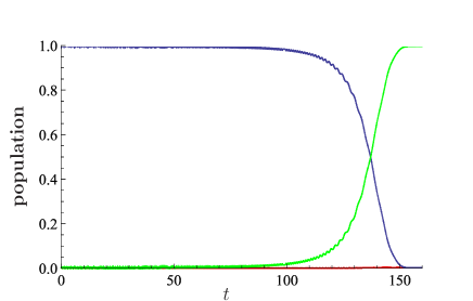
Figure 2: (Color Online) Population of the state $|0\rangle$ (green ascending curve), $|e\rangle$ (red almost constant curve), and $|1\rangle$ (blue descending curve) during the adiabatic transfer under the effect of decoherence at the excited state $|e\rangle$. We have employed parameters $a=0.01\times g$, $\Delta=50\times g$, and $\gamma=0.1\times g$. The results are independent of the value of $g$. The population of state $|1\rangle$ is transferred to the target state $|0\rangle$ with fidelity $0.992$ when the external field is ramped off.

To estimate the effect of dephasing of the adiabatically evolving state due to the decoherence at the excited state, we consider an untransformed initial state $|\psi_{0}\rangle=\frac{1}{\sqrt{2}}|E_{\tilde{\tilde{0}}}\rangle+\frac{1}{\sqrt{2}}|r\rangle$ where $|r\rangle$ denotes a reference state which is not coupled with any other states. Here, we assume that, due to the strong driving field $\frac{g}{\Delta}\ll 1$, the effect of an imperfect initialization is negligible. Since we are interested in an early time stage of the decoherence process, we approximate

$$\tilde{\tilde{\rho}}_{\text{sys},I}(t)\approx\hat{D}_{s}^{\dagger}|\psi_{0}\rangle\langle\psi_{0}|\hat{D}_{s}+\frac{\gamma}{2}\int_{0}^{t}dt^{\prime}[\hat{L}_{I}(t^{\prime}),[\hat{L}_{I}(t^{\prime}),\tilde{\tilde{\rho}}_{\text{sys},I}(0)]],$$

where we substitute $\tilde{\tilde{\rho}}_{\text{sys},I}(t)$ with $\tilde{\tilde{\rho}}_{\text{sys},I}(0)$ in the integrand. We have employed the interaction picture defined for the operators as $\hat{O}_{I}(t)=\hat{U}^{\dagger}_{S}\hat{O}(t)U_{S}(t)$, where $U_{S}(t)=e^{-i\int_{0}^{t}dt^{\prime}\tilde{\tilde{H}}_{\text{sys}}(t^{\prime})}$ is the system time-evolution operator.

Thus, the fidelity can be calculated as follows:

$$F = {}_{S}\langle\psi(t)|\tilde{\tilde{\rho}}_{\text{sys},S}(t)|\psi(t)\rangle_{S}$$ (8)

$$\approx 1-\gamma\int_{0}^{t}|x_{t}|^{2}+O(|x_{t}|^{3})$$

where $|\psi(t)_{\text{}}\rangle_{S}$ denotes the transformed adiabatically evolving state at a time $t$ for vanishing decoherence. Since we have $\frac{g}{\Delta}\ll 1$, $|x_{t}|$ is negligible except for a time region satisfying $0<\Delta\cos^{2}(at)<cg$, where $c$ is some constant. In this time region, we have $0<\frac{\pi}{2a}-t<\frac{n}{a}\sqrt{\frac{g}{\Delta}}$, where $n$ is a constant that depends only on $c$, not on $a$. Hence we obtain $1-F\approx\gamma\int_{\frac{\pi}{2a}-\frac{n}{a}\sqrt{\frac{g}{\Delta}}}^{\frac{\pi}{2a}}|x_{t^{\prime}}|^{2}dt^{\prime}=\frac{1}{2}\gamma\int_{\frac{\pi}{2a}-\frac{n}{a}\sqrt{\frac{g}{\Delta}}}^{\frac{\pi}{2a}}P_{e}dt^{\prime}\leq\frac{25\sqrt{5}}{216}\gamma\frac{n}{a}\sqrt{\frac{g}{\Delta}}\frac{a^{2}\Delta}{g^{3}}$. Therefore we obtain $1-F=O(a)$. As expected, the harmful effect of the decoherence decreases with $a$.

Let us generalize the above results to the two-qubit case. Since we consider independent decoherence processes for the qubits, the master equation for the two-qubit system is $\frac{d\tilde{\tilde{\rho}}_{\text{sys}}}{dt}=\sum_{j=L,R}-i[\tilde{\tilde{H}}^{(j)}_{\text{sys}},\tilde{\tilde{\rho}}_{\text{sys}}]-\frac{\gamma}{2}[\hat{L}_{j},[\hat{L}_{j},\tilde{\tilde{\rho}}_{\text{sys}}]]$. We solve the master equation numerically using the initial state $|M\rangle_{L}|M\rangle_{R}\frac{1}{\sqrt{2}}(\hat{a}^{\dagger}_{L}+\hat{a}^{\dagger}_{R})|\textrm{vac}\rangle$, and show the fidelity $\langle\psi_{\text{Bell}}|\rho_{\textrm{sys}}(\frac{\pi}{2a})|\psi_{\text{Bell}}\rangle$ in Fig. 3. Here, $|\psi_{\text{Bell}}\rangle=\frac{1}{\sqrt{2}}(|M\rangle_{L}|G\rangle_{R}+|G\rangle_{L}|M\rangle_{R})|\text{vac}\rangle$. For reference, we show also the fidelity with neither rotating wave approximation nor transformation corresponding to the superadiabatic basis. The two methods give similar results which verifies that our entanglement generation takes place at high fidelity independent of the theoretical approach. Surprisingly, even when the environmental decoherence rate $\gamma$ is as large as the atom–photon coupling frequency $g$, the protocol still generates high-fidelity entanglement.

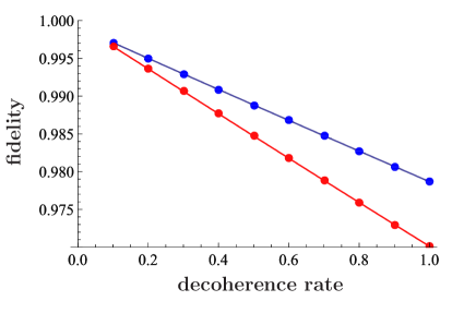
Figure 3: Fidelity of the proposed entanglement generation scheme as a function of the decoherence rate of the environment, $\gamma$, with (top curve) and without (bottom curve) rotating wave approximation. We have fixed the parameters as $a=0.01\times g$, and $\Delta=70\times g$.

Photon loss is one of the major problems in the most of previous entanglement generation protocols Cirac et al. (1999); Lim et al. (2005); Browne et al. (2003); Bose et al. (1999); Feng et al. (2003b); Ladd et al. (2006). In our case, it can also degrade the fidelity since the photon might be lost before coming in the cavity, while in or entering the cavity, or the pulse generated by the single-photon source may fail to provide a photon Lounis and Moerner (2000). The state with photon loss can be described by $\rho_{LR}=(1-P_{\text{loss}})|\psi_{\text{Bell}}\rangle\langle\psi_{\text{Bell}}|+P_{\text{loss}}|M\rangle_{L}|M\rangle_{R}\,{}_{L}\langle M|\,_{M}\langle M|$ even for a perfect adiabatic transfer where $P_{\text{loss}}$ is a probability to lose the photon. Fortunately, this is of the same form as the resource state considered in Refs Campbell and Benjamin (2008); Matsuzaki et al. (2010b); Matsuzaki and Jefferson (2011). If we have an ancillary qubit near the actual qubit at each location, we can perform an efficient two round distillation protocol as follows: It is possible to utilize the state $\rho_{LR}$ as a resource to perform the parity projection on the ancillary qubits. Although this parity projection is imperfect due to the photon loss, by generating the state $\rho_{LR}$ again through another adiabatic transfer, one can utilize the second state for performing the second parity projection on the ancillary qubits in order to obtain a perfect Bell state. The measurement results of the two parity projections let us know whether entanglement between the ancillary qubits is generated or not, and the success probability is calculated $P_{s}=\frac{(1-P_{\text{loss}})^{2}}{2}$ Campbell and Benjamin (2008). Note that the parity projection is one of the most commonly proposed entanglement generation methods Barrett and Kok (2005); Campbell and Benjamin (2008); Matsuzaki et al. (2010b) to make a two dimensional cluster state for quantum computation Raussendorf and Briegel (2001). Moreover, the joint effect of the photon loss and decoherence in this distillation protocol has been studied Matsuzaki and Jefferson (2011), and has been shown to be negligible for weak decoherence. These results show that this distillation protocol makes our scheme robust against the photon loss by using ancillary qubits near the optically active qubits. Such ancillary qubits are available with some species of nanostructures such as the nitrogen–vacancy centers in diamond Dutt et al. (2007); Neumann et al. (2008).

In conclusion, we propose a deterministic scheme to generate entanglement between unstable optically active qubits. Our method is designed to function without the need for photodetectors which are typically major sources of error. With the help of adiabatic transfer, we entangle the qubits without exciting the unstable states, which renders our proposal extremely robust against decoherence. The authors thank T. Close and B. Lovett for useful discussions. We acknowledge Academy of Finland, Emil Aaltonen Foundation, and Centre for International Mobility for financial support.

References

- Cirac et al. (1999) J. I. Cirac, A. K. Ekert, S. F. Huelga, and C. Macchiavello, Phys. Rev. A 59, 4249 (1999).
- Barrett and Kok (2005) S. D. Barrett and P. Kok, Phys. Rev. A 71, 060310 (2005).
- Browne et al. (2003) D. E. Browne, M. B. Plenio, and S. F. Huelga, Phys. Rev. Lett 91, 067901 (2003).
- Bose et al. (1999) S. Bose et al., Phys. Rev. Lett 83, 5158 (1999).
- Feng et al. (2003a) X. L. Feng et al., Phys. Rev. Lett 90, 217902 (2003a).
- Matsuzaki et al. (2010a) Y. Matsuzaki, S. C.Benjamin, and J. Fitzsimons, Phys. Rev. Lett 104, 4 (2010a).
- Matsuzaki et al. (2010b) Y. Matsuzaki, S. Benjamin, and J. Fitzsimons, Phys. Rev. A 82, 010302 (2010b).
- Moehring et al. (2007) D. L. Moehring et al., Nature 449, 68 (2007).
- Kaer and et al (2010) P. Kaer et al., Phys. Rev. Lett. 104, 157401 (2010).
- Gerardot and et al (2008) B. Gerardot et al., Nature 451, 441 (2008).
- Matsuzaki et al. (2010c) Y. Matsuzaki, S. Benjamin, and J. Fitzsimons, arXiv:1009.4171 (2010c).
- Nazir and Barrett (2009) A. Nazir and S. Barrett, Phys. Rev. A 79, 11804 (2009).
- Enk (2005) S. J. van Enk, Phys. Rev. A 72, 064306 (2005).
- Neumann et al. (2009) P. Neumann et al., New J. Phys. 11, 013017 (2009).
- Scully and Zubairy (1997) M. Scully and M. Zubairy, Quantum Optics (Cambridge, 1997).
- Boozer et al. (2007) A. Boozer et al., Phys. Rev. Lett. 98, 193601 (2007).
- Kok and Lovett (2010) P. Kok and B. Lovett, Introduction to optical quantum information processing (Cambridge Univiversity Press, 2010).
- Pekola and et al (2010) J. Pekola et al., Phys. Rev. Lett. 105, 30401 (2010).
- Solinas et al. (2010) P. Solinas et al., Phys. Rev. B 82, 134517 (2010).
- Salmilehto and et al (2010) J. Salmilehto et al., Phys. Rev. A 82, 062112 (2010).
- Messiah (1996) A. Messiah, Quantum mechanics, Wiley, New York (1962).
- Lim et al. (2005) Y. L. Lim, A. Beige, and L. C. Kwek, Phys. Rev. Lett 95, 030505 (2005).
- Feng et al. (2003b) X. L. Feng et al., Phys. Rev. Lett 90, 217902 (2003b).
- Ladd et al. (2006) T. Ladd et al, New J. Phys. 8, 184 (2006).
- Lounis and Moerner (2000) B. Lounis and W. E. Moerner, Nature 407, 491 (2000).
- Campbell and Benjamin (2008) E. T. Campbell and S. C. Benjamin, Phys. Rev. Lett. 101, 130502 (2008).
- Matsuzaki and Jefferson (2011) Y. Matsuzaki and J. H. Jefferson, arXiv:1102.3121 (2011).
- Raussendorf and Briegel (2001) R. Raussendorf and H. Briegel, Phys. Rev. Lett. 86, 5188 (2001).
- Dutt et al. (2007) M. V. G. Dutt et al., Science 316, 1312 (2007).
- Neumann et al. (2008) P. Neumann et al., Science 320, 1326 (2008).