Photoelectron properties of DNA and RNA bases from many-body perturbation theory

Abstract

The photoelectron properties of DNA and RNA bases are studied using many-body perturbation theory within the $GW$ approximation, together with a recently developed Lanczos-chain approach. Calculated vertical ionization potentials, electron affinities, and total density of states are in good agreement with experimental values and photoemission spectra. The convergence benchmark demonstrates the importance of using an optimal polarizability basis in the $GW$ calculations. A detailed analysis of the role of exchange and correlation in both many-body and density-functional theory calculations shows that while self-energy corrections are strongly orbital-dependent, they nevertheless remain almost constant for states that share the same bonding character. Finally, we report on the inverse lifetimes of DNA and RNA bases, that are found to depend linearly on quasi-particle energies for all deep valence states. In general, our $G_{0}W_{0}$-Lanczos approach provides an efficient yet accurate and fully converged description of quasiparticle properties of five DNA and RNA bases.

I INTRODUCTION

Understanding the photoelectron properties of DNA and RNA bases and strands is of central importance to the study of DNA damage following exposure to ultraviolet light or ionizing radiation Colson and Sevilla (1995), and to the development of fast DNA sequencing techniques Zwolak and Di Ventra (2005) and DNA and RNA-based molecular electronics and sensors Porath et al. (2000); Kawai et al. (2009). Extensive experimental efforts Hush and Cheung (1975); Dougherty et al. (1978); Choi et al. (2005); Trofimov et al. (2006); Schwell et al. (2008); Zaytseva et al. (2009); Kostko et al. (2010) have been made since the 1970’s to measure the photoelectron properties of DNA and RNA bases. Meanwhile, theoretical calculations on their ionization potentials and electron affinities have been carried out using density-functional theory (DFT) and high-level quantum chemistry methods Russo et al. (2000); Trofimov et al. (2006); Roca-Sanjuan et al. (2006, 2008); Zaytseva et al. (2009); Bravaya et al. (2010). However, the results from DFT calculations are highly dependent on exchange-correlation functionals, and quantum chemistry methods, though more accurate, require considerably more computational effort. In contrast, many-body perturbation theory within Hedin’s $GW$ approximation Hedin (1965); Hedin and Lundqvist (1969) presents a unique framework that allows access to both quasi-particle (QP) energies and lifetimes on the same footing. This method has been successfully applied to quasi-one-dimensional(1D), two-dimensional (2D) and three-dimensional (3D) semiconductors, insulators, and metals Hybertsen and Louie (1986); Rojas et al. (1995); Rieger et al. (1999); Campillo et al. (1999); Spataru et al. (2001); Onida et al. (2002), and very recently to molecular systems Dori et al. (2006); Tiago et al. (2008); Palummo et al. (2009); Umari et al. (2009, 2010); Stenuit et al. (2010); Umari et al. (2011); Rostgaard et al. (2010); Blase et al. (2011); Faber et al. (2011).

In this work, we present the entire QP spectrum of DNA and RNA bases using many-body perturbation theory within Hedin’s $GW$ approximation, obtained with a recently developed approach that is particularly effective in reaching numerical convergence Umari et al. (2009, 2010). In the $GW$ approximation, the self-energy operator is expressed as a convolution of the QP Green’s function $G$ with the screened Coulomb interaction $W$. Therefore, at increasing system sizes (as is the case for the present work) two computational challenges arise: (i) first, a large basis set has to be adopted to represent operators such as polarizability, and (ii) the calculation of the irreducible dynamical polarizability and that of the self-energy require sums over single-particle conduction states that converge very slowly. We overcome these two obstacles through (i) the use of optimal basis sets for representing the polarization operators Umari et al. (2009) and (ii) the use of a Lanczos-chain algorithm Umari et al. (2010) to avoid explicit sums over empty single-particle states. In addition, the $G_{0}W_{0}$ approximation is adopted, in which the dynamical polarizability is calculated within the random-phase approximation and the QP Green’s function is replaced by its unperturbed single-particle counterpart. This approach is implemented in the open-source Quantum-ESPRESSO distribution Giannozzi et al. (2009). It is applied here to achieve fully converged QP spectra and inverse lifetimes of the five isolated DNA and RNA bases and to investigate the important but distinct roles of exchange and correlation in the $G_{0}W_{0}$ self-energy corrections.

Photoelectron properties of DNA and RNA bases using many-body $GW$ have not been reported until a very recent study by Faber et al.Faber et al. (2011). The work by Faber et al. presents a many-body $GW$ study on QP energies (including ionization potentials and electron affinities) of DNA and RNA bases at several levels of self-consistency within the $GW$ approximation. Their calculations were based on the conventional implementation of the $GW$ method using a localized basis set and a direct sum-over-states approach, and it demonstrated that self-consistent GW calculations indeed further improve the results of $G_{0}W_{0}$ (one-shot $GW$) calculations. Although the localized basis set can significantly improve the computational efficiency and a direct sum-over-states approach can be easily implemented, both of them could have several potential drawbacks, and can introduce large errors in QP energies. One may solve the former issue by systematically increasing the size of basis sets; however, there is no simple solution to the convergence problem introduced by the direct sum-over-state approach. Second, dipole-bound conduction states will not be obtained from localized basis sets due to their highly diffuse character in the vacuum region. In fact, only electron affinities of covalent-bound conduction states were reported in the Faber work. Therefore, it would be desirable to calculate $GW$ QP energies in a plane-wave basis without suffering from the above issues, which is one of the subjects of this research.

The paper is organized as follows. Computational details of our calculations are given in Sec. II. Real-space representations of optimal polarizability basis are displayed in Sec. III. We then report convergence benchmark in Sec. IV. In Sec. V, we present QP energies and inverse lifetimes as well as the entire QP spectra for all five DNA and RNA bases, including guanine (G), adenine (A), cytosine (C), thymine (T), and uracil (U). Vertical ionization potentials (VIPs) and vertical electron affinities (VEAs) are compared to experimental data and other theoretical results. Two types of VEAs are reported using plane-wave basis, including valence-bound (VB, also called covalent-bound) VEA and dipole-bound (DB) VEAs. In Sec. VI, we reveal the role of exchange and correlation in $GW$ self-energy corrections to the DFT Kohn-Sham eigenvalues. Finally, we summarize our work in Sec. VII.

II Computational details

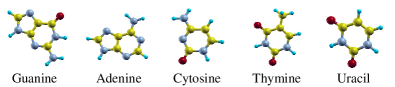
Figure 1: (color online). Ground-state structures of five DNA and RNA bases including G9K-guanine, adenine, C1-cytosine, thymine, and uracil.

Ground-state DFT calculations are performed in a cubic supercell of $18.0^{3}$ Å³, using the Perdew-Burke-Ernzerhof’s (PBE) exchange-correlation functional, Troullier-Martins’s norm-conserving pseudopotentials, and a plane-wave basis set with a cutoff of 544 eV. Structures are optimized with a residual force threshold of 0.026 eV/Å. A truncated Coulomb potential with radius cutoff of 7.4 Å is employed to remove artificial interactions from periodic images. The vacuum level is corrected by an exponential fitting of $E_{\rm HOMO}$ with respect to the supercell volume. The polarizability basis sets have been obtained using a parameter $E^{*}$ of 136.1 eV and a threshold $q^{*}$ of 0.1 a.u., giving an accuracy of 0.05 eV for the calculated QP energies ($E^{*}$ and $q^{*}$ will be explained in the next section). The final accuracy including the errors from the analytic continuation is about 0.05 to 0.1 eV. The structures of five DNA and RNA bases are shown in Fig. 1. Here the effect of gas-phase tautomeric forms Bravaya et al. (2010) of guanine and cytosine on QP properties are beyond the scope of this work, and we only focus on the G9K form of guanine and the C1 form of cytosine Bravaya et al. (2010).

III Optimal polarizability basis

The key quantity in many-body $GW$ calculations is the irreducible dynamic polarizability $\hat{P}_{0}$ in the random-phase approximation:

$$\hat{P}_{0}(\omega)=-i\sum_{v,c}\frac{|\psi_{v}\psi_{c}\rangle\langle\psi_{c}\psi_{v}|}{\omega+i\eta-(\varepsilon_{c}-\varepsilon_{v})},$$ (1)

where $\eta$ is an infinitesimal positive real number. $|\psi_{v}\psi_{c}\rangle$ denotes the direct product of a valence state $\psi_{v}$ and a conduction state $\psi_{c}$ in real space and $\psi_{v}$ and $\psi_{c}$ are considered to be real. A strategy was proposed in Refs. Umari et al., 2009 and Umari et al., 2010 for obtaining a compact basis set, referred to as optimal polarizability basis, to represent $\hat{P}_{0}$ at all frequencies. First, we consider the frequency average of $\hat{P}_{0}(\omega)$ which corresponds to the element at time $t=0$ of its Fourier transform $\tilde{\hat{P}}_{0}(t)$, without considering the constant ($-i$):

$$\tilde{\hat{P}}_{0}(t=0)=\sum_{v,c}|\psi_{v}\psi_{c}\rangle\langle\psi_{c}\psi_{v}|.$$ (2)

We note that $\tilde{\hat{P}}_{0}(t=0)$ is positive definite. Then, the optimal polarizability basis, $\{\Phi_{\mu}\}$, is built from the most important eigenvectors of $\tilde{\hat{P}}_{0}(t=0)$, corresponding to the largest eigenvalues $q_{\mu}$ above a given threshold $q^{*}$:

$$\tilde{\hat{P}}_{0}(t=0)\;|\Phi_{\mu}\rangle=q_{\mu}|\Phi_{\mu}\rangle.$$ (3)

It must be noted that this does not require any explicit calculation of empty (i.e., conduction) states as we can use the closure relation:

$${\hat{P}}_{c}=1-{\hat{P}}_{v},$$ (4)

together with an iterative diagonalization scheme. However, the latter procedure would build polarizability basis sets which are larger than what is necessary for a good convergence of the quasi-particle energy levels. This stems from treating all the one-particle excitations on the same footing, independent of their energy. A practical solution would be to limit the sum in Eq. (2) on the conduction states below a given energy cutoff $E^{*}$:

$$\tilde{\hat{P}}^{\prime}_{0}=\sum_{v,c}^{\epsilon_{c}<E^{*}}|\psi_{v}\psi_{c}\rangle\langle\psi_{c}\psi_{v}|.$$ (5)

However, limiting the sum over the empty states laying in the lower part of the conduction manifold does not allow to use the closure relation alluded to above.

Thus, to keep avoiding the calculation of empty states we replace them in Eq. (5) with a set of plane waves $\{{\mathbf{G}}\}$ with their kinetic energies lower than $E^{*}$, which are first projected onto the conduction manifold using Eq. (4) and then orthonormalized. We indicate these augmented plane-waves as $\{\tilde{\mathbf{G}}\}$ and arrive at the following modified operator:

$$\tilde{\hat{P}}^{\prime\prime}_{0}=\sum_{v,\tilde{\mathbf{G}}}|\psi_{v}\tilde{\mathbf{G}}\rangle\langle\tilde{\mathbf{G}}\psi_{v}|,$$ (6)

which is also positive-definite. An optimal polarizability basis $\{\Phi_{\mu}\}$ is finally obtained by replacing $\tilde{\hat{P}}_{0}(t=0)$ in Eq. (3) with $\tilde{\hat{P}}^{\prime\prime}_{0}$.

It should be stressed that the above approximation is used only for obtaining a set of optimal basis vectors for representing the polarization operators and not for the actual calculation of the irreducible dynamic polarizability at finite frequency in Eq. (1); the latter is performed using a Lanczos-chain algorithm Umari et al. (2010). Moreover, due to the completeness of the eigenvectors of $\tilde{\hat{P}}^{\prime\prime}$, for any value of $E^{*}$ the $GW$ results will converge to the same values by lowering the threshold $q^{*}$, and eventually reach the same results as those obtained by directly using a dense basis of plane-waves. However, compared to the pure plane-waves which are completely delocalized in real space, the optimal polarizability basis is particularly convenient for isolated systems since the most important eigenvectors of $\tilde{\hat{P}}^{\prime\prime}_{0}$ will be mostly localized in the regions with higher electron density. Thus, converged results can be obtained using much smaller optimal-polarizability basis sets than plane-waves basis sets.

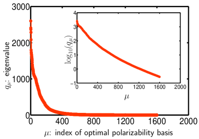
Figure 2: (Color online) Eigenvalue distribution of the optimal polarizability basis for cytosine. The inset plot shows the eigenvalues in a log scale.

Now, we want to have a closer look at the optimal polarizability basis. The eigenvalue distribution of $\tilde{\hat{P}}^{\prime\prime}_{0}$ for cytosine is displayed in Fig. 2. We only show the largest 1600 eigenvalues with $E^{*}=136.1$ eV in the plot, since these provide well converged results. It is clearly seen that the eigenvalues of the optimal polarizability basis decay exponentially and change by almost four orders of magnitude from the first to the last basis. In Fig. 3 we show the real-space representations of a few selected elements. The first five, corresponding to the five largest eigenvalues, are strongly localized around the chemical bonds of the molecule. The second row contains five elements which are more delocalized, and those in the last row are completely delocalized. This indicates that even though localized optimal bases like those shown in the first two rows can be easily captured by localized basis-sets, the delocalized ones with smaller eigenvalues $q_{\mu}$ (like those in the last row) are more difficult to capture if diffuse functions are not employed.

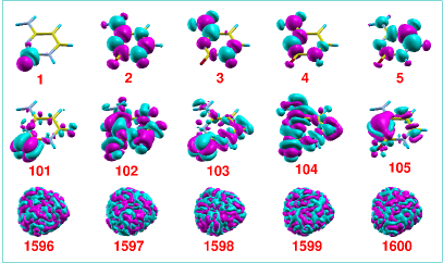
Figure 3: (color online). Real-space representation of optimal-polarizability basis elements for cytosine, labeled with their eigenvalue indexes. Due to the delocalized nature of the optimal basis in the third row, the images in the third row were generated with a smaller isovalue and shown at a larger scale than those in the first two rows.

IV CONVERGENCE BENCHMARK

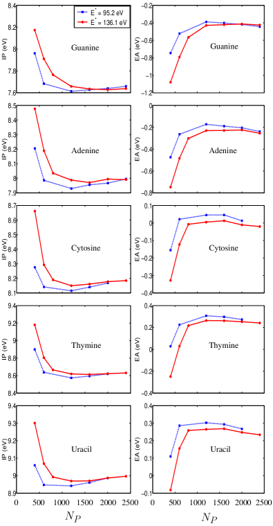
Figure 4: (color online). Convergence benchmark of VIP and VEA of five DNA and RNA bases with respect to the number of optimal-polarizability basis elements $N_{P}$, and augmented plane-wave cutoff $E^{*}$. Results using $E^{*}=$ 95.2 and 136.1 eV are plotted in dashed-blue lines and solid-red lines, respectively.

The number of optimal-polarizability basis elements $N_{P}$ and the energy cutoff of the augmented plane-waves $E^{*}$ are two critical parameters used in our $G_{0}W_{0}$ calculations to achieve both efficiency and accuracy. Therefore, we performed a series of calculations to benchmark the convergence with respect to these two parameters. In Fig. 4, we present the convergence behavior of VIPs and VB-VEAs of five DNA and RNA bases for the highest-occupied molecular orbital (HOMO) and the lowest-unoccupied molecular orbital (LUMO), respectively: ${\rm VIP}\equiv-{\rm Re}(\varepsilon_{\rm HOMO}^{\rm QP})$ and ${\rm VEA}\equiv-{\rm Re}(\varepsilon_{\rm LUMO}^{\rm QP})$. We find that for both VIPs and VEAs convergence within $0.1$ eV is achieved with $\sim 600$ optimal basis elements for $E^{*}=95.2$ eV and with $\sim 750$ optimal basis elements for $E^{*}=136.1$ eV. Indeed, similar trends were reported in Ref. Umari et al., 2009. VIPs and VEAs reported in the following sections are calculated using the most strict parameters ($N_{P}=2400$ and $E^{*}=136.1$ eV).

The above benchmark indicates that, if basis-sets and conduction states in DFT calculations are not properly tested, one could easily obtain non-converged results from $G_{0}W_{0}$ calculations, resulting in higher VIPs and lower VEAs for all five bases. We also note that the choice of $N_{P}$ and $E^{*}$ remains the same for all the DNA and RNA bases, indicating portability for these parameters.

V IONIZATION POTENTIALS AND ELECTRON AFFINITIES

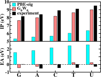
Figure 5: (color online). VIP and VB-VEA of five DNA and RNA bases from our DFT and $G_{0}W_{0}$ calculations. Here we adopt the mean values of various experimental data listed in Table 1. The experimental ranges are $8.0\sim 8.3$, $8.3\sim 8.5$, $8.8\sim 8.9$, $9.0\sim 9.2$, and $9.4\sim 9.6$ eV for G, A, C, T, and U, respectively.

VIPs and VB-VEAs from our $G_{0}W_{0}$ calculations and experimental data are shown in Fig. 5 for all five bases, together with the DFT-PBE eigenvalues for the HOMO and LUMO levels. Only the mean values of experimental VIPs and VEAs are plotted in Fig. 5. $G_{0}W_{0}$ dramatically improves VIPs and VEAs compared to DFT-PBE eigenvalues, providing VIPs of 7.64, 7.99, 8.18, 8.63 and 8.99 eV and VEAs of $-0.43$, $-0.25$, $-0.02$, $0.24$, and $0.23$ eV for G, A, C, T, and U, respectively. The experimental VIPs are compiled in Table 1, and span a range of $8.0\sim 8.3$, $8.3\sim 8.5$, $8.8\sim 8.9$, $9.0\sim 9.2$, and $9.4\sim 9.6$ eV for G, A, C, T, and U. Compared to the mean values of experimental VIPs, the mean absolute error of the calculated VIPs for all five bases is 0.52 eV. Furthermore, experimental VB-VEAs are negative for all five bases, indicating that excited $\pi^{*}$ states are unstable upon electron attachment. This leads to challenging measurements of VEAs and a wide range of measured values Russo et al. (2000); Roca-Sanjuan et al. (2008) listed in Table 1: $-0.56\sim-0.45$, $-0.55\sim-0.32$, $-0.53\sim-0.29$, and $-0.30\sim-0.22$, for A, C, T, and U. Compared to the mean values of experimental VEAs, the mean absolute errors of the calculated VEAs for four bases is 0.45 eV. Interestingly, the VEA of guanine has never been measured successfully, possibly due to a large negative value. This is clearly reflected in our calculated $G_{0}W_{0}$ VEA of $-0.43$ eV, which is the most negative one among all five bases. Even though the $G_{0}W_{0}$ VEAs of thymine and uracil are slightly positive, the trend for all the calculated VEAs agrees well with experiments. In addition, the DFT-PBE HOMO-LUMO gaps for the five bases are about 45% of the $G_{0}W_{0}$ gaps. This is in agreement with previous observations that DFT with the local density approximation (LDA) or the generalized gradient approximation (GGA) of exchange-correlation functionals usually underestimates by 30-50% the true QP energy gap Godby et al. (1986); Gruning et al. (2006).

Table 1: Vertical ionization potentials and vertical electron affinities for several low-lying Kohn-Sham eigenstates close to the HOMO and LUMO levels obtained from negative DFT-PBE eigenvalues and $G_{0}W_{0}$(PBE) in comparison with other $GW$ and quantum chemistry calculations and experimental data. CASPT2: complete active space with second-order perturbation theory; CCSD(T): coupled-cluster with singles, doubles, and perturbative triple excitations; EOM: equation of motion ionization potential coupled-cluster. Only the valence-bound vertical electron affinities are shown in this table. The experimental mean values are taken as the reference in the calculations of mean absolute error(MAE) for both LUMO and HOMO levels.

	DFT-PBE	$G_{0}W_{0}$(PBE)	$G_{0}W_{0}$(LDA)	$GW$(LDA)	CASPT2,/CCSD(T),	EOM	Experiment,,,,
G	[LUMO] 1.12 ($\pi$)	–0.43	–1.04	–1.58	–1.14/
	[HOMO] 5.32 ($\pi$)	7.64	7.49	7.81	8.09/8.09	8.15	8.0$\sim$8.3/8.30/8.26
	5.88 ($n$)	8.67	8.78	9.82	9.56/	9.86	9.90/9.81
	6.37 ($n$)	9.38			9.61/	10.13
	7.04 ($\pi$)	9.43			10.05/	10.29
	6.94 ($\pi$)	9.48			10.24/	10.58	10.45 ($n$)/10.36
	7.76 ($\pi$)	10.37			10.90/	11.38	11.15/11.14
	7.64 ($n$)	10.57
A	[LUMO] 1.81 ($\pi$)	–0.25	–0.64	–1.14	–0.91/		–0.56$\sim$–0.45
	[HOMO] 5.55 ($\pi$)	7.99	7.90	8.22	8.37/8.40	8.37	8.3$\sim$8.5/8.47
	5.89 ($n$)	8.80	8.75	9.47	9.05/	9.37	9.45
	6.65 ($\pi$)	9.06			9.54/	9.60	9.54
	6.74 ($n$)	9.71			9.96/	10.42	10.45
	7.22 ($\pi$)	9.78			10.38/	10.58	10.51
	7.58 ($n$)	10.65			11.06/	11.47	11.35
C	[LUMO] 2.16 ($\pi$)	–0.02	–0.45	–0.91	–0.69/–0.79		–0.55$\sim$–0.32
	[HOMO] 5.67 ($\pi$)	8.18	8.21	8.73	8.73/8.76	8.78	8.8$\sim$9.0/8.89
	5.63 ($n$)	8.50	8.80	9.89	9.42/	9.65	9.45/9.55
	6.28 ($\pi$)	8.94	8.92	9.52	9.49/	9.55	9.89
	6.38 ($n$)	9.39	9.38	10.22	9.88/	10.06	11.20
	8.44 ($\pi$)	11.08			11.84/	12.28	11.64
	9.27 ($\pi$)	11.98			12.71/	13.27	12.93 ($\sigma$, $\pi$)
T	[LUMO] 2.43 ($\pi$)	0.24	–0.14	–0.67	–0.60/–0.65		–0.53$\sim$–0.29
	[HOMO] 6.03 ($\pi$)	8.63	8.64	9.05	9.07/9.04	9.13	9.0$\sim$9.2/9.19
	6.12 ($n$)	8.94	9.34	10.41	9.81/	10.13	9.95$\sim$10.05/10.14
	6.80 ($\pi$)	9.52			10.27/	10.52	10.39$\sim$10.44/10.45
	6.93 ($n$)	9.77			10.49/	11.04	10.80$\sim$10.88/10.89
	8.79 ($\pi$)	11.53			12.37/	12.67	12.10$\sim$12.30/12.27
U	[LUMO] 2.55 ($\pi$)	0.23	–0.11	–0.64	–0.61/–0.64		–0.30$\sim$–0.22
	[HOMO] 6.36 ($\pi$)	8.99	9.03	9.47	9.42/9.43		9.4$\sim$9.6
	6.14 ($n$)	9.07	9.45	10.54	9.83/		10.02$\sim$10.13
	7.00 ($\pi$)	9.68	9.88	10.66	10.41/		10.51$\sim$10.56
	6.92 ($n$)	9.96	10.33	11.48	10.86/		10.90$\sim$11.16
	9.17 ($\pi$)	11.90			12.59/		12.50$\sim$12.70
MAE	[LUMO] 2.64 ($\pi$)	0.45	0.14	0.44	0.30/0.33
	[HOMO] 3.02 ($\pi$)	0.52	0.56	0.15	0.07/0.07	0.05

We further compare several low-lying $G_{0}W_{0}$ VIPs and their excitation characters with experimental and other theoretical results and assignments. First, as shown in Table 1, both $G_{0}W_{0}$ VIPs and their orbital assignments agree well with experiments and other theoretical works for all the five bases, where the corresponding excitation character is either $\pi$ or $n$ (lone pair). Second, our $G_{0}W_{0}$ VIPs, especially those corresponding to the five HOMO levels, are in good agreement with Faber’s $G_{0}W_{0}$ values calculated in localized basis sets. However, larger deviations are clearly observed in some of the lone pair valence states. Their $G_{0}W_{0}$ VIPs are higher than our values by 0.30, 0.40, 0.38, and 0.37 eV for HOMO-1 (the first lone pair state) of cytosine, HOMO-1 (the first lone pair state) of thymine, and HOMO-1 and HOMO-3 (the first and second lone pair states) of uracil, respectively. We plot in Fig. 6 the convergence behavior of VIPs with respect to the dimension of the polarizability basis for these lone pair states to check whether convergence issues are present. But it is apparent that VIPs from our $G_{0}W_{0}$ calculations are fully converged. Another significant difference is found in the valence-bound VEAs for all five LUMO levels. Moreover, Faber’s $G_{0}W_{0}$ VB-VEAs are lower than the present results by 0.61, 0.39, 0.43, 0.38, and 0.34 eV for G, A, C, T, and U, respectively. It is interesting to notice that similar trends of increased VIPs and decreased VEAs are observed in the previous convergence benchmark of Fig. 4, when a small optimal polarizability basis was employed. However, since we do not find significant difference in the $G_{0}W_{0}$ VIPs for other QP states, the source of the above deviations is not clear. Furthermore, as listed in Table 1, the work by Faber et al. demonstrated the importance of self-consistency of QP energies in $GW$ calculations with QP wavefunctions unchanged. This self-consistent $GW$ method increases the $G_{0}W_{0}$ VIPs of the HOMO levels by 0.32, 0.32, 0.52, 0.41, and 0.44 eV and decreases the $G_{0}W_{0}$ VEAs of the LUMO levels by 0.54, 0.50, 0.46, 0.53, and 0.53 eV for G, A, C, T, and U, respectively. Results from advanced quantum chemistry methods are also listed in Table 1, including complete active space with second-order perturbation theory (CASPT2) Roca-Sanjuan et al. (2006, 2008), coupled-cluster with singles, doubles, and perturbative triple excitations [CCSD(T)] Roca-Sanjuan et al. (2006, 2008), and equation of motion ionization potential coupled-cluster (EOM-IP-CCSD) Bravaya et al. (2010). VIPs from CASPT2, CCSD(T), and EOM-IP-CCSD for the HOMO levels are very similar, and close to the experimental mean values within 0.07, 0.07, and 0.05 eV, respectively. VEAs from CASPT2 and CCSD(T) for the LUMO levels are also close to each other; however, they are less close to the mean experimental values (within 0.30 and 0.33 eV, respectively). Among all the theoretical approaches, self-consistent $GW$ and quantum chemistry methods provide the VIPs and VEAs with the smaller errors with respect to the experimental data.

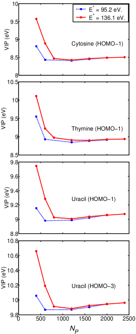
Figure 6: (color online). Convergence behavior of vertical ionization potentials of several $n$ states in DNA and RNA bases with respect to the number of optimal polarizability basis, $N_{P}$, and augmented plane-wave cutoff, $E^{*}$. These states are cytosine’s HOMO-1 state, thymine’s HOMO-1 state, and uracil’s HOMO-1 and HOMO-3 states. Results using $E^{*}=$ 95.2 and 136.1 eV are plotted in dashed-blue lines and solid-red lines, respectively.

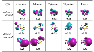
Figure 7: (color online). Valence-bound and dipole-bound VEAs and their corresponding QP states, calculated at the DFT-PBE level, in the five DNA and RNA bases. Values listed below are VEAs in the unit of eV.

Beside the VB-VEAs, there also exist dipole-bound (DB) VEAs, which correspond to having the additional electron weakly bound to the DNA and RNA bases by local electrostatic dipoles Roca-Sanjuan et al. (2008). Both types of QP states are shown in Fig. 7. It is clear that all five VB states are localized $\pi^{*}$ states, while DB states present large lobes, highly extended outside the molecules. These lobes are mainly located in the vicinity of the N-H bond, and with a non-negligible dipole moment along their bond axis. The energy difference between the VB-VEAs and their nearest DB-VEAs, $\Delta_{\rm VEA}\equiv$ VEA(VB) $-$ VEA(DB), are –0.23, 0.06, 0.21, 0.48, and 0.52 eV for G, A, C, T, and U, respectively. This suggests that at the $G_{0}W_{0}$ level VB states in the latter four bases are energetically more stable than the DB ones.

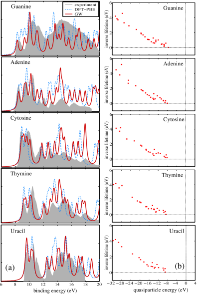
Figure 8: (color online). (a) Experimental valence photoemission spectrum (shaded gray area), DFT-PBE DOS (blue dashed lines), and $G_{0}W_{0}$ DOS (red solid lines). Both DOS curves are shifted to match the first VIP of experimental data. Experimental PES spectra of G, A, C, T, and U are extracted from Refs. Lin et al., 1980, Trofimov et al., 2006, Trofimov et al., 2006, Trofimov et al., 2006, and Odonnell et al., 1980, respectively. The theoretical DOS have been obtained through a Lorentzian broadening defined by a width of $0.4$ eV. (b) $G_{0}W_{0}$ QP energies and inverse lifetime for valence states (unit: eV).

Experimental valence photoemission spectra extends into deep valence states Lin et al. (1980); Odonnell et al. (1980); Trofimov et al. (2006), allowing us to further evaluate our $G_{0}W_{0}$ results at a broader energy range. The DFT-PBE and $G_{0}W_{0}$ densities of states (DOS) for all five bases, neglecting any oscillator strength effect, are compared to valence photoemission spectra in Fig. 8(a). For better comparison, both curves are shifted to match the first experimental VIP. It is clearly shown that for all five bases the $G_{0}W_{0}$ DOS agrees much better with the experiment than the DFT-PBE DOS, thanks to the correct relative position of the various peaks. Moreover, the $G_{0}W_{0}$ self-energy not only leads to large corrections to DFT eigenvalues, but also provides an estimation of QP intrinsic lifetimes due to inelastic electron-electron scattering, as reflected in the imaginary part of QP energies, with $1/\tau_{n}=2|{\rm Im}(\varepsilon_{n}^{\rm QP})|$. The calculated QP inverse lifetimes at the $G_{0}W_{0}$ level are plotted in Fig. 8(b) against the corresponding QP valence energies. Although $G_{0}W_{0}$ permits only a rough estimate of QP lifetimes (the exact ones are expected to be zero in the range $[2{\rm Re}(\varepsilon_{\rm HOMO}^{\rm QP}),\;{\rm Re}(\varepsilon_{\rm HOMO}^{\rm QP})]$), we note that the QP inverse lifetimes decrease almost linearly with respect to QP energies for the deep valence states in all five cases. However, it is still unknown to what extent the $G_{0}W_{0}$ estimation of inverse lifetime would be modified by fully self-consistent $GW$ calculations.

VI ROLE OF EXCHANGE AND CORRELATION IN GROUND-STATE DFT AND $GW$ CALCULATIONS

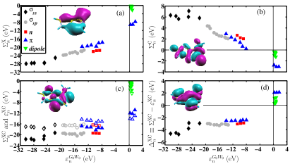
Figure 9: (color online). The role of exchange and correlation in the $G_{0}W_{0}$ self-energy corrections to Kohn-Sham eigenvalues of 25 valence states and 10 conduction states in adenine. (a) $G_{0}W_{0}$ exchange energy $\Sigma_{n}^{\rm X}$, (b) $G_{0}W_{0}$ correlation energy $\Sigma_{n}^{\rm C}$, (c) the sum of $G_{0}W_{0}$ exchange and correlation energy $\Sigma_{n}^{\rm XC}$ (filled symbols) and DFT XC energy $\varepsilon_{n}^{\rm XC}$ (unfilled symbols), and (d) the difference between $G_{0}W_{0}$ and DFT exchange-correlation energy, $\Delta_{n}^{\rm XC}\equiv\Sigma_{n}^{\rm XC}-\varepsilon_{n}^{\rm XC}$. Four types of molecular orbitals are illustrated in (a)–(d), corresponding to $\sigma_{ss}$, $\sigma_{sp}$, $n$, and $\pi$ characters.

To understand the role of exchange and correlation in the self-energy corrections to the DFT-PBE results, we first express each Kohn-Sham eigenvalue $\varepsilon_{n}^{\rm KS}$ of eigenstate $\psi_{n}$ for the $n$-th state as the sum of a single-particle energy $\varepsilon_{n}^{\rm S}$ and an exchange-correlation energy $\varepsilon_{n}^{\rm XC}$: $\varepsilon_{n}^{\rm KS}=\varepsilon_{n}^{\rm S}+\varepsilon_{n}^{\rm XC}$, where $\varepsilon_{n}^{\rm S}$ contains the energy contributions from the kinetic energy operator, the external ionic potential, and the Hartree term. Furthermore, the $G_{0}W_{0}$ QP energy can be written in terms of the exchange self-energy $\Sigma_{n}^{\rm X}$ and of the correlation self-energy $\Sigma_{n}^{\rm C}$: $\varepsilon_{n}^{\rm G_{0}W_{0}}=\varepsilon_{n}^{\rm S}+\Sigma_{n}^{\rm X}+\Sigma_{n}^{\rm C}$. Exchange and correlation effects can then be systematically investigated by analyzing $\Sigma_{n}^{\rm X}$, $\Sigma_{n}^{\rm C}$, $\Sigma_{n}^{\rm XC}$, $\varepsilon_{n}^{\rm XC}$, and $\Delta_{n}^{\rm XC}$, with $\Sigma_{n}^{\rm XC}\equiv\Sigma_{n}^{\rm X}+\Sigma_{n}^{\rm C}$ and $\Delta_{n}^{\rm XC}\equiv\Sigma_{n}^{\rm XC}-\varepsilon_{n}^{\rm XC}$. We consider the adenine molecule and plot the above quantities with respect to the $G_{0}W_{0}$ QP energy $\varepsilon_{n}^{G_{0}W_{0}}$. As shown in Figs. 9(a) and (b), the $G_{0}W_{0}$ exchange energy $\Sigma_{n}^{\rm X}$ increases from $-28.0$ to $-17.8$ eV for the 25 valence states and from $-9.2$ to $-0.2$ eV for the 10 conduction states, while the $G_{0}W_{0}$ correlation energy $\Sigma_{n}^{\rm C}$ decreases from 7.1 down to 0.2 eV for the valence states and from $-0.3$ to $-3.1$ eV for the conduction states. This clearly shows that $\Sigma_{n}^{\rm X}$ is always negative, stabilizing both electron and hole excitations; however, $\Sigma_{n}^{\rm C}$ is positive for valence states and negative for conduction states, indicating that the effect of correlation is that of destabilizing hole excitations and of stabilizing electron excitations. Although $\Sigma_{n}^{\rm X}$ and $\Sigma_{n}^{\rm C}$ have opposite trends for hole excitations, exchange interactions eventually dominate due to their larger magnitude, leading to the negative $\Sigma_{n}^{\rm XC}$ of Fig. 9(c). Interestingly, the $G_{0}W_{0}$ $\Sigma_{n}^{\rm XC}$ is lower than the DFT-PBE $\varepsilon_{n}^{\rm XC}$ for the valence states, but higher than $\varepsilon_{n}^{\rm XC}$ for the conduction states. Consequently, the difference $\Delta_{n}^{\rm XC}$ between $\Sigma_{n}^{\rm XC}$ and $\varepsilon_{n}^{\rm XC}$, shown in Fig. 9(d), is negative for the valence manifold and positive for the conduction manifold, resulting in an increased HOMO-LUMO gap. The same behavior is observed for the other four bases as well.

As shown in Fig. 9, we can recognize five major orbital types among the valence and conduction orbitals of the isolated adenine molecule: $\sigma_{ss}$, $\sigma_{sp}$, $n$, $\pi$, and dipole-bound states. The lowest six states correspond to $\sigma$ orbitals due to $s$-$s$ hybridization, which have larger $G_{0}W_{0}$ exchange, correlation, and total self-energy corrections than the other states. The following ten states at higher energy levels exhibit $\sigma_{sp}$ character, and their $\Sigma_{n}^{\rm X}$ and $\Sigma_{n}^{\rm C}$ show a linear but opposite dependence with respect to the $G_{0}W_{0}$ QP energy $\varepsilon_{n}^{G_{0}W_{0}}$. Thus, their sum $\Sigma_{n}^{\rm XC}$ is shown to be almost constant, ranging from $-20.5$ to $-19.4$ eV. Since the same trend is present in $\varepsilon_{n}^{\rm XC}$, the final difference $\Delta_{n}^{\rm XC}$ between $G_{0}W_{0}$ and DFT results stays almost constant, between $-3.3$ and $-3.0$ eV. The next three $n$ and six $\pi$ valence states and three $\pi^{*}$ conduction states have a similar behavior, despite different magnitudes in their self-energy corrections. In particular, the six $\pi$ valence states are lowered by about $-2.5$ eV, while the three $\pi^{*}$ conduction states are lifted by 2.1 eV, leading to an increase of 4.6 eV for the HOMO-LUMO gap. The above observations provide an important evidence that the $G_{0}W_{0}$ self-energy corrections are highly orbital-dependent and on average $\Sigma^{\rm X}(\sigma_{ss})<\Sigma^{\rm X}(\sigma_{sp})<\Sigma^{\rm X}(n)<\Sigma^{\rm X}(\pi)$, $\Sigma^{\rm C}(\sigma_{ss})>\Sigma^{\rm C}(\sigma_{sp})>\Sigma^{\rm C}(n)>\Sigma^{\rm C}(\pi)$, and $\Delta^{\rm XC}(\sigma_{ss})<\Delta^{\rm XC}(\sigma_{sp})\approx\Delta^{\rm XC}(n)<\Delta^{\rm XC}(\pi)$. Consequently, the commonly-used “scissor operator” to correct bandgaps by rigidly lowering the valence levels and increasing the conduction levels by the same amount will never be adequate for describing the entire QP spectrum.

VII SUMMARY

In summary, VIPs, VEAs, and DOS of five DNA and RNA bases obtained from a fully converged many-body $G_{0}W_{0}$ approach are found to be in very good agreement with experiments and other theoretical works. Two types of vertical electron affinities are found, corresponding to localized valence-bound excitations and delocalized dipole-bound excitations. Our calculations further reveal that QP inverse lifetimes depend linearly on QP energies for the deep valence states. They, however, come from the zero-th order $G_{0}W_{0}$ estimation, and may be significantly affected in self-consistent $GW$ calculations. Interestingly, the $G_{0}W_{0}$ self-energy corrections are highly orbital dependent, but remain relatively constant for the states with similar bonding character. Moreover, $G_{0}W_{0}$ VIPs of lone pair states deviate from the experimental ones more than those for $\pi$ states. Whether this difference comes from the different self-interaction errors in Kohn-Sham eigenstates will require further studies using self-interaction corrected functionals Perdew and Zunger (1981); Dabo et al. (2010); Korzdorfer (2011); work is in progress along this direction.