Medium Access Control for Wireless Networks with Peer-to-Peer State Exchange

Abstract

Distributed medium access control (MAC) protocols are proposed for wireless networks assuming that one-hop peers can periodically exchange a small amount of state information. Each station maintains a state and makes state transitions and transmission decisions based on its state and recent state information collected from its one-hop peers. A station can adapt its packet length and the size of its state space to the amount of traffic in its neighborhood. It is shown that these protocols converge to a steady state, where stations take turns to transmit in each neighborhood without collision. In other words, an efficient time-division multiple access (TDMA) like schedule is formed in a distributed manner, as long as the topology of the network remains static or changes slowly with respect to the execution of the protocol.

I Introduction

In most wireless networks, medium access control (MAC) is needed to avoid excessive collisions, which occur if a station transmits to another transmitting station, which is half-duplex, or a station receives multiple simultaneous transmissions and cannot successfully decode the desired message(s). Many MAC protocols can be viewed as requiring each station to maintain a state, which determines when the station transmits. To provide distributed operation, this state is updated based on information available locally in space. For example, in carrier-sense multiple access (CSMA) protocols, the state is determined by the carrier sensing operation and the random backoff mechanism.

This paper considers MAC protocols in which stations explicitly exchange limited state information. The protocols are self-stabilizing, i.e., they converge to a collision-free schedule regardless of the initial state. The underlying network is assumed to be static or vary slowly with respect to the execution of the MAC protocol. In the steady state, these protocols behave like time-division multiple access (TDMA), in which stations take turns to transmit without collision; while in the transient state, they behave like CSMA, such that stations contend with each other, trying to find a slot for transmission and avoid collisions. Under the assumption of a single collision domain, i.e., all stations can hear each other, self-stabilizing MAC protocols have been studied in [1, 2, 3]. By learning transmission decisions of others, stations are able to find a collision-free schedule in a decentralized manner. As is pointed out in [1], these protocols cannot guarantee the formation of a collision-free schedule in case of multiple collision domains and focus on schedules for unicast traffic.

This paper focuses on establishing collision-free schedules for broadcast and multicast traffic in networks with multiple collision domains. It is well-known that multiple collision domains complicate scheduling due in part to hidden terminals and exposed terminals. For unicast traffic, state exchange in the form of RTS/CTS signaling can help alleviate these complications. However, this is not suitable when a station wants to broadcast a packet to all nearby stations. To facilitate this, we consider a richer form of state exchange.

We build on work in [4] and [5], which introduces self-stabilizing MAC protocols for one- and two-dimensional regular networks on lattices. The technique is to divide time into periodic cycles, where each cycle is divided into slots. A station maintains a single state and transmits only over the slot corresponding to its state. Once the protocols converge, a periodic state pattern (with immediate neighbors assuming different states) is formed throughout the regular network, and the maximum broadcast throughput is achieved. If one directly applies these ideas to networks with arbitrary topologies, sufficiently many states are needed for stations with many neighbors, but in a neighborhood with few stations, the wireless channel is underutilized because few states are occupied.

There has been a significant work on MAC scheduling for networks that builds on the seminal max-weight algorithm [6], and attempts to derive distributed, low complexity algorithms which approach the throughput-optimal performance of [6]. Examples include [7, 8, 9, 10, 11, 12]. These approaches seek to adapt the resulting schedule to queue variations. Here, we instead consider a model with saturated traffic and seek to find fixed rate-based schedules, as in [13]. Such a schedule is naturally more useful for traffic that has a fixed long-term arrival rate. More bursty traffic can be accomodated by reserving some fraction of time for contention-based access as in [14].

The main contributions of this paper are as follows:

1. In Section II, we introduce the concept of multiple resolutions, i.e., a station having more neighbors uses a fine resolution (more states in its state space, each state corresponding to a shorter slot); while a station with fewer neighbors uses a coarse resolution (fewer states in its state space, each state corresponding to a longer slot).

2. In Sections III and IV, multi-resolution MAC protocols are proposed for broadcast in one- and two- dimensional networks with arbitrary topologies, respectively. These protocols guarantee every station a chance to transmit in each cycle. In addition, they achieve approximate proportional fairness in the sense that a station’s throughput is approximately inversely proportional to the node density in its neighborhood. We show that in one-dimensional networks, stations can determine their resolutions in a distributed manner. The same also holds for two-dimensional networks under a mild condition. In case the condition is not met, we propose a mechanism for stations to dynamically change their resolutions until collisions do not occur in the entire network.

3. We show that the multi-resolution protocols can be applied to a more general setting. In Section V, we consider multicast traffic. In Section VI, broadcast and multicast in networks with multiple orthogonal channels are considered.

In all cases, the convergence of such protocols to a collision-free schedule is rigorously established. To achieve the global optimum in terms of throughput is an NP-complete problem [15, 16], which is out of scope of this paper.

II System Model

Consider a simple model for wireless networks where two stations have a direct radio link between them if they can hear each other. The network can be modeled by an arbitrary graph $G=(V,A)$, where $V=\{\mathbf{r}_{i}\}_{i=0}^{\lvert V\rvert-1}$ is the set of stations labeled by their coordinates, and $A=\{(\mathbf{r}_{i},\mathbf{r}_{j})\}\subset V\times V$ is the set of undirected links. Let $V_{\mathbf{r}}$ denote the set of (one-hop) peers or neighbors of station $\mathbf{r}$. We assume the interference range of a station is the same as its transmission range, so $V_{\mathbf{r}}$ denotes both the set of potential receivers and interferers for station $\mathbf{r}$. Sections III and IV study the case where every station broadcasts packets to all its one-hop peers in a single channel. Section V studies the case where every station multicasts packets to a certain subset of its one-hop peers in a single channel. In Section VI, broadcast and multicast in networks with multiple orthogonal channels are considered. For both broadcast and multicast, saturated traffic is assumed.

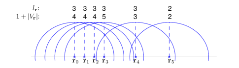
Figure 1: A multi-resolution MAC protocol in a one-dimensional network. In 1, there are $6$ stations at positions $\mathbf{r}_{0},\dots,\mathbf{r}_{5}$. The half circles represent the transmission ranges of the stations. The values of $1+\lvert V_{\mathbf{r}}\rvert$ and $l_{\mathbf{r}}$ for different stations are shown on top of the corresponding circles. A possible schedule over a cycle is shown in 1.

Next we formalize the concept of multiple resolutions. Let time be divided into cycles of fixed length. We let station $\mathbf{r}$ decide on a resolution represented by an integer $l_{\mathbf{r}}\geq 0$. From the viewpoint of this station, each cycle is further divided into $2^{l_{\mathbf{r}}}$ slots of equal length. The state of this station in the $t$-th cycle, denoted by $X_{\mathbf{r}}(t)$, is a binary string of length $l_{\mathbf{r}}$ corresponding to the index of the slot in the $t$-th cycle over which the station transmits. Let $\boldsymbol{X}(t)=\{X_{\mathbf{r}}(t)\}_{\mathbf{r}\in V}$ be the configuration in the $t$-th cycle. We assume that all stations are synchronized. A finer resolution can be obtained by ‘splitting’ or ‘refining’ a coarse resolution. We assume that packets transmitted by a station fit in a slot of its own resolution. Stations using coarse resolutions can also transmit multiple packets of smaller sizes in a slot.

A collision occurs between two one-hop or two-hop peers if they transmit at the same time. Mathematically, two such stations $\mathbf{r}_{i}$ and $\mathbf{r}_{j}$, with $l_{\mathbf{r}_{i}}\leq l_{\mathbf{r}_{j}}$ (without loss of generality), collide in the $t$-th cycle when

$$\text{the binary string }X_{\mathbf{r}_{i}}(t)\text{ is a prefix of }X_{\mathbf{r}_{j}}(t).$$ (1)

In a collision-free configuration, (1) must not hold for any pair of one-hop and two-hop peers. Consider the example described in Fig. 1. Station $\mathbf{r}_{5}$ uses state $10$, i.e., it transmits during the third quarter of the cycle. Station $\mathbf{r}_{3}$ uses state $101$ with a finer resolution consisting of eight states, so that it transmits in the sixth slot of the cycle which is divided into $8$ slots. Station $\mathbf{r}_{3}$’s resolution can be seen as a refinement of that of station $\mathbf{r}_{5}$. Since $10$ is a prefix of $101$, and stations $\mathbf{r}_{3}$ and $\mathbf{r}_{5}$ are two-hop peers as shown in Fig. 1, these two stations collide (at receiver $\mathbf{r}_{4}$).

We assume that at the end of each cycle, each station acquires the current states of its one-hop and two-hop peers, error-free. Such message exchanges can be carried out either over a control channel or over a dedicated time period. The careful reader may object that this itself requires a collision-free schedule. However, since this control information is relatively low-rate, we assume that other techniques can be utilized for sending it. For example, stations can use a random access scheme to exchange the short control messages. Alternatively, the rapid on-off division duplex (RODD) scheme in [17, 18] can be used here, which enables all stations to exchange their control messages simultaneously. From now on, we will assume stations exchange state information within a control frame orthogonal to data frames in time or in frequency.

Let stations choose their next states based only on the current states of their one-hop and two-hop peers and themselves. The state process of the MAC protocol can be modeled as a Markov Chain of Markov Fields (MCMF) [19], i.e., a process for which the states $\boldsymbol{X}=\{\boldsymbol{X}(t)\}_{t\in\mathbb{N}}$ satisfy

• $\boldsymbol{X}(1),\boldsymbol{X}(2),\dots$ is a Markov chain, and

• for every $t$, $\boldsymbol{X}(t)$ is a Markov field conditioned on $\boldsymbol{X}(t-1)$.

In fact, $\boldsymbol{X}(t)$ consists of independent random variables conditioned on $\boldsymbol{X}(t-1)$ in our case. Here, we only consider protocols in which stations make identically distributed decisions conditioned on the same previous states of their one-hop and two-hop peers and themselves.

In Sections III and IV we measure the performance by the one-hop broadcast throughput $\rho_{\text{BC}}$, which is the average proportion of time a station receives packets in each cycle. A station receives a packet if and only if it does not transmit and only one of its peers transmits. If there is no collision,

$$\rho_{\text{BC}}=\frac{1}{\lvert V\rvert}\sum_{\mathbf{r}\in V}\sum_{\mathbf{r}^{\prime}\in V_{\mathbf{r}}}2^{-l_{\mathbf{r}^{\prime}}}=\frac{1}{\lvert V\rvert}\sum_{\mathbf{r}\in V}\lvert V_{\mathbf{r}}\rvert 2^{-l_{\mathbf{r}}}.$$ (2)

The two expressions are obtained by counting throughput from the receiver side and the transmitter side, respectively. In Section V, we use the one-hop multicast throughput $\rho_{\text{MC}}$ to measure the performance. In this case, a station receives a packet if and only if it does not transmit, only one of its peers transmits and it is an intended receiver for the packet. Let $D_{\mathbf{r}}\subseteq N_{\mathbf{r}}$ denote the set of intended receivers of the multicast by $\mathbf{r}$. If there is no collision, the one-hop multicast throughput is,

$$\rho_{\text{MC}}=\frac{1}{\lvert V\rvert}\sum_{\mathbf{r}\in V}\sum_{\mathbf{r}^{\prime}\colon\mathbf{r}\in D_{\mathbf{r}^{\prime}}}2^{-l_{\mathbf{r}^{\prime}}}=\frac{1}{\lvert V\rvert}\sum_{\mathbf{r}\in V}\lvert D_{\mathbf{r}}\rvert 2^{-l_{\mathbf{r}}}.$$ (3)

It should be noted that under the concept of multiple resolutions, the structure of the states can be more complex than that described here. For example, the states may be represented by tertiary codes, so the number of slots in a cycle need not be a power of $2$. Also, to represent collisions using the prefix condition (1), it is not required that all slots in a cycle must have the same length; the only requirements are that all slot boundaries of a coarse resolution are also slot boundaries of a fine resolution, and two slots overlap in time if and only if the states representing the slots satisfy the prefix condition.

III Broadcast in One-Dimensional Networks

III-A Determining the number of states

We first consider one-dimensional networks, i.e., all stations lie on a straight line. We further assume the following: if $\mathbf{r}_{i}$ and $\mathbf{r}_{j}$ are one-hop peers, then all stations located between $\mathbf{r}_{i}$ and $\mathbf{r}_{j}$ are also one-hop peers of both $\mathbf{r}_{i}$ and $\mathbf{r}_{j}$. To avoid collision, a station and all its one-hop peers must transmit at different times. The following result shows that a station can determine its resolution solely based on the size of the largest one-hop neighborhood that it belongs to.

Theorem 1

Suppose in a one-dimensional network, each station shares the number of stations within its one-hop neighborhood (i.e., $1+|V_{\mathbf{r}}|$ for station $\mathbf{r}$) with all its one-hop peers, then collision-free configurations are guaranteed to exist by letting stations choose their resolutions according to

$$l_{\mathbf{r}}=\biggl{\lceil}\log_{2}\biggl{(}\max_{\mathbf{r}^{\prime}\in V_{\mathbf{r}}\cup\{\mathbf{r}\}}(1+\lvert V_{\mathbf{r}^{\prime}}\rvert)\biggr{)}\biggr{\rceil}.$$ (4)

The resulting one-hop broadcast throughput is given by (2), where $l_{\mathbf{r}}$ in (2) is specified in (4).

Fig. 1 illustrates the procedure in Theorem 1. Each station computes the size of its one-hop neighborhood (which is labeled on top of the half circle representing its transmission range). Stations then choose their resolutions following (4).

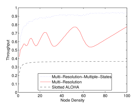
Figure 2: Throughput of one-dimensional networks versus node density.

Consider finite segments of one-dimensional networks where stations are distributed following a Poisson point process with node density $\lambda$. We assume that the network is a unit disk graph with transmission range $R=1$, i.e., there is a link between two stations if and only if the distance between them is at most equal to the transmission range $R=1$. We evaluate the throughput by averaging over $100$ different realizations of the networks. How the throughput $\rho_{\text{BC}}$ varies with the node density $\lambda$ is shown in Fig. 2. The throughput oscillation is due to the fact that the size of any state space is a power of $2$. In a worst-case scenario, if a station determines that it needs $2^{l}+1$ states, it has to use a resolution of $2^{l+1}$ states, meaning that almost half of the cycle will be left idle, hence the throughput is close to $0.5$. Thus, a small increase in the node density may cause a rather large drop in the throughput under certain circumstances.

After forming a collision-free configuration, there may still be many idle slots in certain neighborhoods. To illustrate this, consider a collision-free configuration which is formed by letting stations, from the left to the right, pick the earliest slot to transmit such that they do not collide with any station. We then let stations, from the left to the right, reclaim the idle slots to transmit, such that station $\mathbf{r}$ reclaims at most $\Bigl{\lceil}\frac{2^{l_{\mathbf{r}}}}{\lvert V_{\mathbf{r}}\rvert}\Bigr{\rceil}-1$ additional slots and ensures that it does not collide with other stations. By doing so, station $\mathbf{r}$ transmits at a rate approximately equal to $\frac{1}{\lvert V_{\mathbf{r}}\rvert}$. The top curve in Fig. 2 shows that a significant improvement in throughput results from this reclaiming.

For comparison, we also compute the throughput for slotted ALOHA in a one-dimensional network, where stations use the same fixed transmission probability $p$ but do not exchange any state information. Consider a segment of a one-dimensional network of length $2R$ with a station at the center. This station has $k$ peers with probability $\exp(-\lambda 2R)\frac{(\lambda 2R)^{k}}{k!}$, and receives a packet successfully with probability $kp(1-p)^{k}$. Then,

$$\rho_{\text{BC}}(p) = \sum_{k=1}^{\infty}\exp(-\lambda 2R)\frac{(\lambda 2R)^{k}}{k!}kp(1-p)^{k}$$

$$= \lambda 2Rp(1-p)\exp(-\lambda 2Rp).$$

The maximum throughput is

$$\rho_{\text{BC}}=\frac{\lambda 2R}{2+\sqrt{4+(\lambda 2R)^{2}}}\exp\Biggl{(}-\frac{2\lambda 2R}{2+\lambda 2R+\sqrt{4+(\lambda 2R)^{2}}}\Biggr{)}$$

which is achieved with transmission probability

$$p=\frac{2}{2+\lambda 2R+\sqrt{4+(\lambda 2R)^{2}}}.$$

This optimized throughput, with $R=1$, is plotted in Fig. 2. The multi-resolution MAC protocol provides $46.7\%$ to $112.2\%$ improvement in terms of throughput over slotted ALOHA.

III-B Multi-Resolution MAC Protocol

In the following we propose a multi-resolution protocol that leads to a collision-free configuration starting from an arbitrary initial configuration. Stations can learn two-hop state information in each cycle as follows. In the $t$-th cycle, station $\mathbf{r}$ collects $\bigl{\{}X_{\mathbf{r}^{\prime}}(t)\bigr{\}}_{\mathbf{r}^{\prime}\in V_{\mathbf{r}}}$, and then broadcasts $\bigl{\{}X_{\mathbf{r}^{\prime}}(t)\bigr{\}}_{\mathbf{r}^{\prime}\in V_{\mathbf{r}}\cup\{\mathbf{r}\}}$. Hence, station $\mathbf{r}$ knows $X_{\mathbf{r}^{\prime}}(t)$ for all one-hop and two-hop peers $\mathbf{r}^{\prime}$ (this is accomplished by letting station $\mathbf{r}$ broadcast $2l_{\mathbf{r}}+\sum_{\mathbf{r}^{\prime}\in V_{\mathbf{r}}}l_{\mathbf{r}^{\prime}}$ bits), and selects its state at the $(t+1)$-st cycle following Protocol 1, where the parameter $\epsilon$ is set to 0 in the case of one-dimensional networks (in case of two-dimensional networks discussed in Section IV, we will set $\epsilon$ to a strictly positive number).

Protocol 1 Multi-Resolution MAC Protocol for Broadcast

1:  while station $\mathbf{r}$ is active do

2:        $\mathbf{r}$ sets the votes on all states to zero.

3:        for $\mathbf{r}^{\prime}\in V_{\mathbf{r}}\cup\{\mathbf{r}\}$ do

4:              if $\mathbf{r}$ is the only station occupying its current state in station $\mathbf{r}^{\prime}$’s one-hop neighborhood then

5:                    $\mathbf{r}$’s current state is assigned a single vote of weight one.

6:              else

7:                    $\mathbf{r}$ determines which states (according to $\mathbf{r}$’s resolution) are idle or have collisions in $\mathbf{r}^{\prime}$’s one-hop neighborhood.

8:                    A vote of weight $\frac{1}{n}$ is added to each such state, where $n$ is the number of such states.

9:              end if

10:        end for

11:        if $n_{s}>0$ for multiple $s$’s, where $n_{s}$ is the total weight state $s$ receives then

12:              Replace $n_{s}$ by $n_{s}+\epsilon$, where $\epsilon\geq 0$, for all $s$.

13:        end if

14:        $\mathbf{r}$ selects state $s$ with a probability proportional to $f(n_{s})$.

15:  end while

In Protocol 1, $f:\mathbb{R}\mapsto\mathbb{R}$ can be any increasing function with $f(0)=0$. Empirically, a good choice is $f(n_{s})=\exp(Jn_{s})\mathbf{1}_{\{n_{s}>0\}}$, where $\mathbf{1}_{\{\cdot\}}$ is the indicator function and $J>0$ is the strength of interaction (more on this later). The idea of Protocol 1 is that a station ‘reserves’ a slot for a peer if it knows that this peer does not collide with other peers, and notifies any peer experiencing collisions to stay away from these ‘reserved’ slots. We have the following convergence result for this protocol.

Theorem 2

If each station in a one-dimensional network chooses its resolution following Theorem 1 and executes Protocol 1, then all stations will converge to a collision-free configuration, regardless of the initial state. The resulting throughput is given in Theorem 1.

Proof:

Using Protocol 1, if a station does not collide with any one-hop or two-hop peers, then all the votes will be given to its current state, and it will remain in its current state with probability one. Therefore, if the current configuration is collision-free, then the same configuration will appear in every subsequent cycle, so every collision-free configuration is absorbing. Hence we only need to consider the case when the current configuration is not collision-free and show that such configuration is transient. To do this we explicitly construct a collision-free configuration, which the stations in the current configuration can transition to with positive probability.

Without loss of generality, assume the stations are indexed such that $\mathbf{r}_{i}$ is on the left of $\mathbf{r}_{j}$ if and only if $i<j$. Stations take turns to find a state that is collision-free with all stations on their left:

• Station $\mathbf{r}_{0}$ remains in its initial state, so it is collision-free with all stations on its left (notice that following Protocol 1, every station has a nonzero probability of remaining in the same state).

• Now, assume stations $\mathbf{r}_{0},\dots,\mathbf{r}_{i-1}$ are collision-free with all stations on their left. For station $\mathbf{r}_{i}$:

  1. If its current state is collision-free with all stations on its left (including the special case where there is no neighboring station on its left), then it remains in its current state.

  2. Otherwise, consider the farthest left one-hop peer of station $\mathbf{r}_{i}$, which we denote by $\mathbf{r}_{j}$. If $\mathbf{r}_{i}$ collides with some station $\mathbf{r}_{k}$ on its left, then $\mathbf{r}_{j}$ must be able to detect it, because $\mathbf{r}_{j}$ must be one-hop peers of both $\mathbf{r}_{i}$ and $\mathbf{r}_{k}$ ($\mathbf{r}_{j}$ and $\mathbf{r}_{k}$ can be the same station). $\mathbf{r}_{j}$ and all one-hop peers $\mathbf{r}_{m}$ of $\mathbf{r}_{j}$ use resolutions of at least $2^{\lceil\log_{2}(1+\lvert V_{\mathbf{r}_{j}}\rvert)\rceil}$ states. Therefore, from station $\mathbf{r}_{j}$’s point of view, there are at most $\lvert V_{\mathbf{r}_{j}}\rvert$ distinct busy periods, each of length at most $2^{-\lceil\log_{2}(1+\lvert V_{\mathbf{r}_{j}}\rvert)\rceil}$. This means that there is at least one idle slot according to $\mathbf{r}_{j}$’s resolution, i.e., none of the $\mathbf{r}_{m}$’s use that slot. Therefore, $\mathbf{r}_{j}$ gives a vote of nonzero weight on this slot to $\mathbf{r}_{i}$, then with nonzero probability, $\mathbf{r}_{i}$ chooses this slot (or a fraction of this slot if it uses a finer resolution) and becomes collision-free with all stations on its left.

Finally, when station $\mathbf{r}_{\lvert V\rvert-1}$ finds a state that is collision-free with all stations on its left, the configuration is now collision-free. Therefore, all configurations with collisions are transient, proving both Theorems 1 and 2. ∎

III-C Simulations: Convergence Speed-up by Annealing

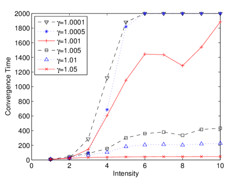
(a) Convergence time

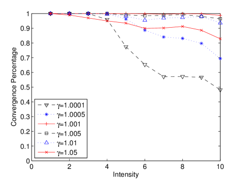
(b) Convergence percentage

Figure 3: Simulations of the multi-resolution protocol with annealing for one-dimensional networks.

Simulations of the proposed protocol show that it may take a long time for a collision-free configuration to appear. Here we propose speeding up the convergence by annealing, i.e., we consider the multi-resolution protocol with $f(n_{s})=\exp(J(t)n_{s})\mathbf{1}_{\{n_{s}>0\}}$, where $J(t)=\gamma J(t-1)$, $\gamma>1$ controls the increase in the strength of interaction, and $J(0)=1$. Define the convergence time to be the first time that a certain configuration is observed and remains unchanged till the end of the simulation, and the convergence percentage to be the proportion of stations that do not collide with other stations in that configuration. This configuration may not be collision-free. This means that there is a nonzero probability that the network transits to another configuration, but this probability is so small (as $J(t)$ is very large, resulting in every station staying in the state with maximum vote) that this transition is practically impossible. We consider a line segment of length $50$ on which stations are distributed following a Poisson point process with node density $\lambda$. The network is a unit disk graph with transmission range $R=1$. Ten simulations are run for each combination of $\lambda$ and $\gamma$. All simulations last for $2000$ iterations. The convergence time and percentage are plotted in Figs. 3(a) and 3(b) respectively. When $\gamma$ is too small, the effect of annealing is not significant, and as shown the algorithm may not have converged after $2000$ iterations. When $\gamma$ is too large, the convergence time is reduced drastically, but the proportion of stations experiencing collisions is still significant. Notice the similarity of the results here with the annealing process in statistical mechanics: when the annealing is too slow, it takes longer time to reach the state with minumum energy; when the annealing is too fast, the system reaches some metastable state or becomes glassy with noncrystalline structure.

IV Broadcast in Two-Dimensional Networks

IV-A Determining the number of states

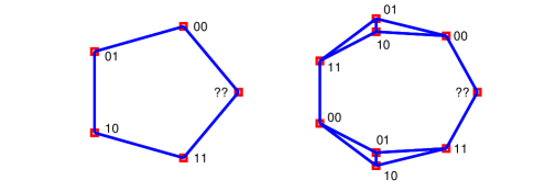
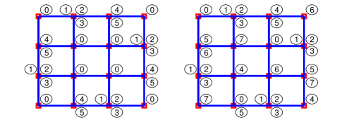
Figure 4: Intricacies for two-dimensional networks: 4 determining the number of states (‘??’ labels stations that are unable to pick a state without collision), 4 converging to a collision-free configuration.

Unlike in one-dimensional networks, the resolution $l_{\mathbf{r}}$ cannot be completely determined by (4) in two-dimensional networks. An example is shown in the left part of Fig. 4. If (4) is used here, every station has two one-hop peers and therefore should use a resolution of four states. But since every station is within two hops of every other station, at least five states are needed to resolve any collision. For a two-dimensional network, the following theorem shows that (4) gives a lower bound on the needed resolution. An upper bound on the resolution is also given.

Theorem 3

A lower bound on the needed resolution for a collision-free configuration for broadcast to exist is given by

$$\underline{l}_{\mathbf{r}}=\biggl{\lceil}\log_{2}\biggl{(}\max_{\mathbf{r}^{\prime}\in V_{\mathbf{r}}\cup\{\mathbf{r}\}}(1+\lvert V_{\mathbf{r}^{\prime}}\rvert)\biggr{)}\biggr{\rceil}.$$ (5)

A corresponding upper bound is given by

$$\overline{l}_{\mathbf{r}}=\biggl{\lceil}\log_{2}\biggl{(}\max_{\mathbf{r}^{\prime}\in V_{\mathbf{r}}^{2}\cup\{\mathbf{r}\}}(1+\lvert V_{\mathbf{r}^{\prime}}^{2}\rvert)\biggr{)}\biggr{\rceil},$$ (6)

where $V_{\mathbf{r}}^{2}$ is the set of one-hop or two-hop peers of $\mathbf{r}$. The resulting one-hop broadcast throughput of a two-dimensional network is bounded as follows:

$$\frac{1}{\lvert V|}\sum_{\mathbf{r}\in V}\lvert V_{\mathbf{r}}\rvert 2^{-\overline{l}_{\mathbf{r}}}\leq\rho_{\text{BC}}\leq\frac{1}{\lvert V|}\sum_{\mathbf{r}\in V}\lvert V_{\mathbf{r}}\rvert 2^{-\underline{l}_{\mathbf{r}}}.$$ (7)

Proof:

For a station to receive a packet from each one-hop peer, the station itself and all its one-hop peers must transmit at different times. If $\mathbf{r}^{\prime}\in V_{\mathbf{r}}\cup\{\mathbf{r}\}$, station $\mathbf{r}$ is within the one-hop neighborhood $V_{\mathbf{r}^{\prime}}\cup\{\mathbf{r}^{\prime}\}$, and therefore $1+\lvert V_{\mathbf{r}^{\prime}}\rvert$ states are required to resolve any collision in $V_{\mathbf{r}^{\prime}}\cup\{\mathbf{r}^{\prime}\}$. Then, at least $\max_{\mathbf{r}^{\prime}\in V_{\mathbf{r}}\cup\{\mathbf{r}\}}(1+\lvert V_{\mathbf{r}^{\prime}}\rvert)$ states are required. Finally, we assume $\underline{l}_{\mathbf{r}}$ to be an integer and $2^{\underline{l}_{\mathbf{r}}}\geq\max_{\mathbf{r}^{\prime}\in V_{\mathbf{r}}\cup\{\mathbf{r}\}}(1+\lvert V_{\mathbf{r}^{\prime}}\rvert)$, therefore the lower bound (5) is established.

Observe that a station cannot transmit when one of its one-hop or two-hop peers transmits in a collision-free configuration. In the worst case, at most one station in every two-hop neighborhood transmits at any time. Now, if $\mathbf{r}^{\prime}\in V_{\mathbf{r}}^{2}\cup\{\mathbf{r}\}$, station $\mathbf{r}$ is within the two-hop neighborhood $V_{\mathbf{r}^{\prime}}^{2}\cup\{\mathbf{r}^{\prime}\}$, and in the worst case $1+\lvert V_{\mathbf{r}^{\prime}}^{2}\rvert$ states are required to resolve any collision in $V_{\mathbf{r}^{\prime}}^{2}\cup\{\mathbf{r}^{\prime}\}$. Therefore, at most $\max_{\mathbf{r}^{\prime}\in V_{\mathbf{r}}^{2}\cup\{\mathbf{r}\}}(1+\lvert V_{\mathbf{r}^{\prime}}^{2}\rvert)$ states are required. Finally, we assume $\overline{l}_{\mathbf{r}}$ to be an integer and $2^{\overline{l}_{\mathbf{r}}}\geq\max_{\mathbf{r}^{\prime}\in V_{\mathbf{r}}^{2}\cup\{\mathbf{r}\}}(1+\lvert V_{\mathbf{r}^{\prime}}^{2}\rvert)$, therefore the upper bound (6) is established. ∎

The upper bound in Theorem 3 can be quite loose. When the network $G$ is ‘well-connected’ it can be improved on by using the maximum clique in $G^{2}$ containing $\mathbf{r}$, where $G^{2}=(N,A^{2})$ is the square of $G$, i.e., $(\mathbf{r}_{i},\mathbf{r}_{j})\in A^{2}$ if $\mathbf{r}_{i}$ and $\mathbf{r}_{j}$ are one-hop or two-hop peers in $G$. More formally, we require that $G^{2}$ to be chordal, meaning that in any cycle of at least four vertices, there must exist an edge between some pair of nonadjacent vertices. A key property of chordal graphs is that they have a perfect elimination ordering of their vertices [21], i.e., one can order the vertices by repeatedly finding a vertex such that all its neighbors form a clique, and then removing it along with all incident edges. We use this property to prove the next theorem, which shows that the choice of $l_{\mathbf{r}}$ based on the maximum clique size in $G^{2}$ is adequate.

Theorem 4

Suppose a two-dimensional network $G$ has a chordal square, i.e., $G^{2}$ is chordal. If station $\mathbf{r}$ uses resolution $l_{\mathbf{r}}=\lceil\log_{2}\lvert C_{\mathbf{r}}\rvert\rceil$, where $C_{\mathbf{r}}$ is the maximum clique in $G^{2}$ containing $\mathbf{r}$, then it is possible for each station to choose a state such that collision-free configurations exist.

Proof:

By assumption, there exists a perfect elimination ordering of vertices for $G^{2}$. Without loss of generality, assume the stations are indexed following the reverse of the perfect elimination ordering, i.e., $\mathbf{r}_{j}$ appears after $\mathbf{r}_{i}$ in the perfect elimination ordering if and only if $j<i$. We will show by induction that station $\mathbf{r}_{i}$ must be able to find a state so that it is collision-free with stations $\mathbf{r}_{j}$ where $j<i$.

Station $\mathbf{r}_{0}$ can pick any state. Now, assume stations $\mathbf{r}_{0},\dots,\mathbf{r}_{i-1}$ pick their states such that they are collision-free among themselves. Then, for station $\mathbf{r}_{i}$, let $C=\{\mathbf{r}_{j}\colon j<i\text{ and }(\mathbf{r}_{i},\mathbf{r}_{j})\in A^{2}\}$. By definition of perfect elimination ordering, $C\cup\{\mathbf{r}_{i}\}$ is a clique in $G^{2}$. Therefore, $\mathbf{r}_{i}$ and all $\mathbf{r}_{j}\in C$ use resolutions of at least $2^{\lceil\log_{2}(1+\lvert C\rvert)\rceil}$ states. Hence, from station $\mathbf{r}_{i}$’s point of view, there are $\lvert C\rvert$ distinct busy periods, each of length at most $2^{-\lceil\log_{2}(1+\lvert C\rvert)\rceil}$. This means that there is at least one idle slot according to $\mathbf{r}_{i}$’s resolution, i.e., none of the $\mathbf{r}_{j}$’s in $C$ use that slot. Therefore, station $\mathbf{r}_{i}$ can pick this slot (or a fraction of this slot if it uses a finer resolution) and therefore becomes collision-free with all stations $\mathbf{r}_{j}$ where $j<i$. Repeating this argument, when station $\mathbf{r}_{\lvert V\rvert-1}$ finds a state that is collision-free with stations $\mathbf{r}_{j}$ where $j<\lvert V\rvert-1$, then the configuration is now collision-free. ∎

The condition in Theorem 4 is sufficient but not necessary. For example, the right part of Fig. 4 shows that a collision-free configuration cannot be found using the resolutions predicted in Theorem 3. Consider also the right part of Fig. 4, which is a $4\times 4$ square lattice where multiple stations are collocated on some lattice points. Theorem 3 predicts that every station uses a resolution of eight states, and a collision-free configuration exists, as shown in the figure. For illustrative purposes, we use decimal representation of the states, e.g., state $101$ is denoted as $5$. In both cases, $G^{2}$ is not chordal.

Since the sizes of all state spaces are powers of $2$, additional states are provisioned in many cases. Therefore, a collision-free configuration is likely to exist by using the rule in Theorem 4 even for many networks without chordal squares.

IV-B Multi-resolution MAC Protocol for Two-dimensional Networks

Protocol 1 with $\epsilon=0$ does not always work for all two-dimensional networks. In particular, the resulting Markov chain can have an absorbing class with more than one configuration, none of which is collision-free. An example is illustrated in Fig. 4. Every station uses a resolution of eight states. The right part of Fig. 4 shows that a collision-free configuration exists. But, if the initial configuration is the one shown in the left part of Fig. 4, and the protocol in Section III is used, then the following occurs:

1. All stations in initial states $1,2,3,4,5$ remain in their current states with probability one, since they do not cause any collision. All stations in initial state $0$ can only choose $0,6,7$ as their next states, because all other states are not available. This repeats for all subsequent iterations.

2. Consider the four stations in the middle of the network, which have initial states $0$. They are within two hops of each other, so they must use different states. However, only states $0,6,7$ are available to them in any cycle. Hence, collision-free configurations cannot be reached.

Choosing $\epsilon>0$ in Protocol 1 prevents the preceding deadlock. For any station, if the votes received do not all point to a single state, then the station increases the total weight of the votes received for any state by a nonzero constant. A station in this situation will have nonozero probability of choosing any state to be its next state. This randomization does not affect any absorption configuration, and is necessary to establish the counterpart of Theorem 2 for two-dimensional networks.

Theorem 5

For a two-dimensional network, suppose each station uses a sufficiently fine resolution (e.g., the upper bound in Theorem 3), so that the existence of collision-free configurations is guaranteed. Then, starting from an arbitrary initial configuration, Protocol 1 with $\epsilon>0$ will converge to a collision-free configuration.

Proof:

As in the proof of Theorem 2, every collision-free configuration is absorbing. So we only need to consider the case when the initial configuration is not collision-free.

The remaining proof is similar to the proof of Theorem 1 in [22]. We will show that an all-zero configuration, i.e., a configuration where every station’s state is a binary string of all zeros, is reached with nonzero probability, and then in the next cycle there is a nonzero probability of reaching a collision-free configuration. Without loss of generality, assume station $\mathbf{r}_{0}$ collides with some station. Consider a spanning tree rooted at $\mathbf{r}_{0}$, and assume the stations are indexed following the breadth-first search order. Using Protocol 1 with $\epsilon>0$, the following happens with nonzero probability:

• Station $\mathbf{r}_{0}$ chooses a state that collides with its child with the smallest index in the spanning tree, and repeats this for all children in the spanning tree following the breadth-first search ordering in subsequent cycles. After colliding with all children, it then chooses the all-zero state and remains in that state.

• For station $\mathbf{r}_{i}$:

  1. If it does not collide with its parent in the spanning tree, then it remains in its current state until it collides with its parent.

  2. When it collides with its parent, it follows what station $\mathbf{r}_{0}$ does, i.e., it chooses a state that collides with its child with the smallest index in the spanning tree, and repeats this for all children in the spanning tree following the breadth-first search ordering in subsequent cycles. After colliding with all children, it then chooses the all-zero state and remains in that state.

Finally, all stations are in the all-zero state, i.e., every station collides with all one-hop and two-hop peers. Therefore, in the next cycle, there is a nonzero probability that the stations choose any configuration including one that is collision-free, where the existence of collision-free configurations is guaranteed. Hence, all configurations with collisions are transient. ∎

IV-C Simulations: Dynamically Adjusting the Number of States

For a general two-dimensional network, it is difficult for stations to predict the resolutions they need. It may still be difficult even for networks with chordal squares, since it is not known whether it is possible to find the maximum clique in the square of a graph efficiently. Therefore, we propose the following dynamic algorithm. Initially, every station sets its resolution to be the lower bound given by Theorem 3 and executes the modified multi-resolution protocol with annealing. If a station knows that the local configuration within its two-hop neighborhood remains the same for a number of iterations ($10$ in our simulations), but it still experiences collisions, then it checks if there are any idle states within its two-hop neighborhood. If such states exist, it selects one of these states; otherwise, it doubles the size of its state space (i.e., it ‘refines’ its resolution), picks its state randomly, resets the strength of interaction it uses and continues executing the protocol. The refinement stops once the local configuration is collision-free, or the upper bound given by Theorem 3 is reached, whichever occurs first. The upper bound provides a guarantee on the minimum rate a station can have.

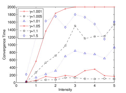
(a) Convergence time

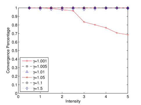
(b) Convergence percentage

Figure 5: Simulations of the multi-resolution protocol with annealing for two-dimensional networks.

For simulation, we consider a $10\times 10$ square area of two-dimensional networks where stations are distributed following a Poisson point process with node density $\lambda$. All other simulation settings are the same as those for one-dimensional networks. The convergence time and percentage are plotted in Figs. 5(a) and 5(b), respectively. The convergence time is longer compared to one-dimensional networks, since stations may need to adjust their resolutions. When $\gamma$ is too large, the convergence time increases drastically. In this case, the interaction between stations is so large that the protocol behaves like majority vote shortly after the protocol is executed. This makes the randomization of states after each refinement not effective in resolving collisions.

V Extension to Multicast

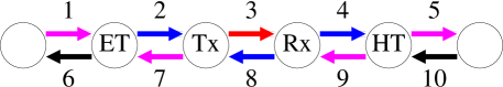
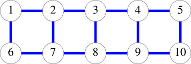
Figure 6: 6 Multicast on a graph $G$ is equivalent to 6 broadcast on the corresponding auxiliary graph $G^{L}$.

In this section we extend the results to multicast traffic. Here, we consider every undirected link in the network $G$ to be two directed links in opposite directions. We define two directed links $a,a^{\prime}$ in $G$ to be (one-hop) link-peers if and only if the transmitter of one link is the receiver of the other link. The neighboring relationship can be represented by an auxiliary graph $G^{L}$ constructed as follows: a directed link $a$ in $G$ is represented by a vertex $a$ in $G^{L}$, and two directed links $a,a^{\prime}$ being one-hop link-peers in $G$ is represented by an undirected edge $(a,a^{\prime})$ in $G^{L}$. An example is shown in Fig. 6. Suppose station Tx transmits packets to station Rx only, i.e., only link $3$ is used by Tx, and suppose it is active. Then all its one-hop link-peers (links $2,4,8$) must be silent due to the half-duplex constraint. All two-hop link-peers must be silent also, because either they are originated from hidden terminals (links $1,5,9$), or they are links not used by Tx (link $7$). All other links are free to transmit, because either they are links from exposed terminals to other stations not interfered by Tx (link $6$), or they are sufficiently far away (link $10$). Therefore, under this neighboring model, a link must choose a state different from any of its one-hop and two-hop link-peers in order to form a collision-free configuration. Correspondingly, in the auxiliary graph $G^{L}$, when vertex $3$ is active, its one-hop and two-hop peers must be silent at the same time. In general, if we associate a state variable to each link, which always takes the same value as the state variable of the transmitter of the link (meaning that all links used by the same multicast session must be in the same state), then multicast on a graph $G$ is equivalent to broadcast on the corresponding auxiliary graph $G^{L}$. Therefore, most results obtained for broadcast in previous sections can be applied here with slight modifications.

As discussed in Section II, we assume station $\mathbf{r}$ multicasts packets to a subset $D_{\mathbf{r}}$ of its one-hop peers. We represent a multicast session by the set of links used, i.e., $M_{\mathbf{r}}=\{(\mathbf{r},\mathbf{r}^{\prime})\colon\mathbf{r}^{\prime}\in D_{\mathbf{r}}\}$. Following the ideas in Section IV, we use one-hop and two-hop link-neighborhood size to estimate the lower and upper bounds on the resolution for multicast.

Theorem 6

A lower bound on the needed resolution for a collision-free configuration for multicast to exist is computed as follows:

$$\underline{I}_{a} = \{\mathbf{r}^{\prime}\colon M_{\mathbf{r}^{\prime}}\cap(L_{a}\cup\{a\})\neq\emptyset\},$$ (8)

$$\underline{l}_{a} = \max_{a^{\prime}\in L_{a}\cup\{a\}}\lvert\underline{I}_{a^{\prime}}\rvert,$$ (9)

$$\underline{l}_{\mathbf{r}} = \biggl{\lceil}\log_{2}\biggl{(}\max_{a\in M_{\mathbf{r}}}\underline{l}_{a}\biggr{)}\biggr{\rceil},$$ (10)

where $L_{a}$ is the set of one-hop link-peers of link $a$, and $\underline{I}_{a}$ contains the multicast sessions that use any link within link $a$’s one-hop link-neighborhood. A corresponding upper bound is computed as follows:

$$\overline{I}_{\mathbf{r}} = \{\mathbf{r}^{\prime}\colon M_{\mathbf{r}^{\prime}}\cap\cup_{a\in M_{\mathbf{r}}}(L_{a}^{2}\cup\{a\})\neq\emptyset\},$$ (11)

$$\overline{l}_{\mathbf{r}} = \biggl{\lceil}\log_{2}\biggl{(}\max_{\mathbf{r}^{\prime}\in\overline{I}_{\mathbf{r}}}\lvert\overline{I}_{\mathbf{r}^{\prime}}\rvert\biggr{)}\biggr{\rceil},$$ (12)

where $L_{a}^{2}$ is the set of one-hop or two-hop link-peers of link $a$, and $\overline{I}_{\mathbf{r}}$ contains $M_{\mathbf{r}}$ and all multicast sessions that cannot be active at the same time as $M_{\mathbf{r}}$ because they use links within the two-hop link-neighborhood of a link used by $M_{\mathbf{r}}$. The resulting one-hop multicast throughput of a two-dimensional network is bounded as follows:

$$\frac{1}{\lvert V\rvert}\sum_{\mathbf{r}\in V}\lvert D_{\mathbf{r}}\rvert 2^{-\overline{l}_{\mathbf{r}}}\leq\rho_{\text{MC}}\leq\frac{1}{\lvert V\rvert}\sum_{\mathbf{r}\in V}\lvert D_{\mathbf{r}}\rvert 2^{-\underline{l}_{\mathbf{r}}}.$$ (13)

Proof:

For any link $a$, at most one multicast session in $\underline{I}_{a}$ can be active at any time. Therefore, at least $\lvert\underline{I}_{a}\rvert$ states are required to resolve collisions among the multicast sessions in $\underline{I}_{a}$. Link $a$ belongs to the one-hop link-neighborhood of any link $a^{\prime}\in L_{a}\cup\{a\}$. Therefore, if link $a$ is used by any multicast session, it needs at least $\max_{a^{\prime}\in L_{a}\cup\{a\}}\lvert\underline{I}_{a^{\prime}}\rvert=\underline{l}_{a}$ states to resolve collisions. Finally, station $\mathbf{r}$ should use the finest resolution that its links use, therefore we have the lower bound (10).

For any station $\mathbf{r}$, at most one multicast session in $\overline{I}_{\mathbf{r}}$ can be active at any time in the worst case. Therefore, at most $\lvert\overline{I}_{\mathbf{r}}\rvert$ states are required to resolve collisions among the multicast sessions in $\overline{I}_{\mathbf{r}}$. Finally, station $\mathbf{r}$ also belongs to $\overline{I}_{\mathbf{r}^{\prime}}$ for $\mathbf{r}^{\prime}\in\overline{I}_{\mathbf{r}}$, implying the upper bound (12). ∎

Note that Theorem 6 gives the same result as Theorem 3 when there is only broadcast, since $\underline{I}_{a}=V_{\mathbf{r}}\cup\{\mathbf{r}\}$ when $\mathbf{r}$ is the transmitter of link $a$, and $\overline{I}_{\mathbf{r}}=V_{\mathbf{r}}^{2}\cup\{\mathbf{r}\}$.

The corresponding multi-resolution MAC protocol for multicast is shown as Protocol 2. The only difference from Protocol 1 is that the votes on station $\mathbf{r}$’s next state are cast by using the state information of link $a^{\prime}$’s one-hop link-neighborhood (lines $3$ and $6$), where $a^{\prime}$ belongs to any one-hop link-neighborhood of link $a$ used by station $\mathbf{r}$ (line $2$). By considering the analogy between multicast on $G$ and broadcast on $G^{L}$, we have the following convergence result.

Protocol 2 Multi-Resolution MAC Protocol for Multicast

1:  while station $\mathbf{r}$ is active do

2:        $\mathbf{r}$ sets the votes on all states to zero.

3:        for $a^{\prime}\in\cup_{a\in M_{\mathbf{r}}}(L_{a}\cup\{a\})$ do

4:              if $\mathbf{r}$ is the only station occupying its current state in link $a^{\prime}$’s one-hop link-neighborhood then

5:                    $\mathbf{r}$’s current state is assigned a single vote of weight one.

6:              else

7:                    $\mathbf{r}$ determines which states (according to $\mathbf{r}$’s resolution) are idle or have collisions in link $a^{\prime}$’s one-hop link-neighborhood.

8:                    A vote of weight $\frac{1}{n}$ is added to each such state, where $n$ is the number of such states.

9:              end if

10:        end for

11:        if $n_{s}>0$ for multiple $s$’s, where $n_{s}$ is the total weight state $s$ receives then

12:              Replace $n_{s}$ by $n_{s}+\epsilon$, where $\epsilon>0$, for all $s$.

13:        end if

14:        $\mathbf{r}$ selects state $s$ with a probability proportional to $f(n_{s})$.

15:  end while

Theorem 7

For multicast on a two-dimensional network, suppose each station uses a sufficiently fine resolution (e.g., the upper bound in Theorem 6), so that the existence of collision-free configurations is guaranteed. Then, starting from an arbitrary initial configuration, Protocol 2 will converge to a collision-free configuration.

Next we discuss how station $\mathbf{r}$ exchanges the state information required in Protocol 2. A naive scheme is to let stations code the state information of different links into separate messages. However, links having the same transmitter share some common state information. Therefore, we introduce the following two-step message exchange which exploits this redunduncy to reduce the amount of information exchange between stations.

The first step is to compute the state information of link $a$’s one-hop link-neighborhood for all $a$ such that $\mathbf{r}$ is the transmitter of link $a$, i.e., $a=(\mathbf{r},\mathbf{r}^{\prime})$. In the $t$-th cycle, station $\mathbf{r}$ collects $\bigl{\{}X_{\mathbf{r}^{\prime}}(t)\bigr{\}}_{\mathbf{r}^{\prime}\in V_{\mathbf{r}}}$. Then $\mathbf{r}$ constructs the following disjoint sets:

1. common state information: $\mathcal{C}_{\mathbf{r}}(t)=\{X_{\mathbf{r}^{\prime\prime}}(t)\}_{\mathbf{r}^{\prime\prime}\colon\mathbf{r}\in D_{\mathbf{r}^{\prime\prime}}}$ (this includes the states of one-hop peers of $\mathbf{r}$ having $\mathbf{r}$ as an intended receiver, notice this state information is common to all links having $\mathbf{r}$ as the transmitter);

2. self state information: $\mathcal{S}_{\mathbf{r}}(t)=\{X_{\mathbf{r}}(t)\}$ (this includes $\mathbf{r}$’s state, notice this state information is common only to all links in $M_{\mathbf{r}}$);

3. link-specific state information for $(\mathbf{r},\mathbf{r}^{\prime})$ where $\mathbf{r}^{\prime}\in V_{\mathbf{r}}$: $\mathcal{L}_{\mathbf{r},\mathbf{r}^{\prime}}(t)=\{X_{\mathbf{r}^{\prime}}(t)\}$ if $\mathbf{r}\notin D_{\mathbf{r}^{\prime}}$, and $\mathcal{L}_{\mathbf{r},\mathbf{r}^{\prime}}(t)=\emptyset$ otherwise (this includes $\mathbf{r}^{\prime}$’s state if $\mathbf{r}^{\prime}$ transmits to stations other than $\mathbf{r}$.

For $a=(\mathbf{r},\mathbf{r}^{\prime})$, if $a\in M_{\mathbf{r}}$, the union $\mathcal{C}_{\mathbf{r}}(t)\cup\mathcal{S}_{\mathbf{r}}(t)\cup\mathcal{L}_{\mathbf{r},\mathbf{r}^{\prime}}(t)$ is the state information in the one-hop link-neighborhood of link $a$; otherwise if $a\notin M_{\mathbf{r}}$, the corresponding state information is the union $\mathcal{C}_{\mathbf{r}}(t)\cup\mathcal{L}_{\mathbf{r},\mathbf{r}^{\prime}}(t)$. As an example, consider the network shown in Fig. 7. A solid arrow is a link between a transmitter and an intended receiver, while a dashed arrow is a link between a transmitter and a nonintended receiver. Fig. 7 shows how station $\mathbf{r}_{0}$ computes the state information of links $a_{1},a_{2},a_{3},a_{4}$ following the above procedure. Since $\mathbf{r}_{0}$ is an intended receiver for both $\mathbf{r}_{2}$ and $\mathbf{r}_{3}$, the states of both $\mathbf{r}_{2}$ and $\mathbf{r}_{3}$ are common to all links $a_{1},a_{2},a_{3},a_{4}$, hence $\mathcal{C}_{\mathbf{r}_{0}}(t)=\{X_{\mathbf{r}_{2}},X_{\mathbf{r}_{3}}\}$. Because $\mathbf{r}_{0}$ transmits to $\mathbf{r}_{1}$ and $\mathbf{r}_{2}$ only, $\mathcal{S}_{\mathbf{r}_{0}}(t)=\{X_{\mathbf{r}_{0}}\}$ is the state information common only to links $a_{1},a_{2}$. Since $\mathbf{r}_{1}$ and $\mathbf{r}_{4}$ transmit to stations other than $\mathbf{r}_{0}$, $X_{\mathbf{r}_{1}}$ and $X_{\mathbf{r}_{4}}$ are included in $\mathcal{L}_{\mathbf{r}_{0},\mathbf{r}_{1}}(t)$ and $\mathcal{L}_{\mathbf{r}_{0},\mathbf{r}_{4}}(t)$, respectively.

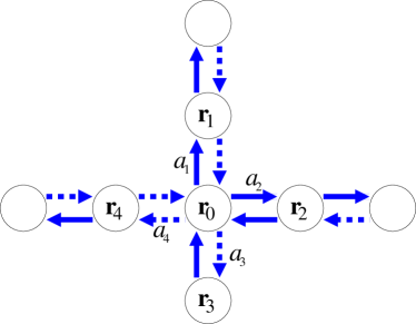
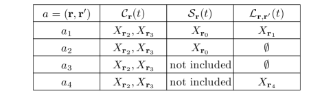
Figure 7: One-hop state information of links $a_{1},a_{2},a_{3},a_{4}$ with station $\mathbf{r}_{0}$ being the transmitter.

The second step is to let $\mathbf{r}$ broadcast $\mathcal{C}_{\mathbf{r}}(t)$, $\mathcal{S}_{\mathbf{r}}(t)$, and $\mathcal{L}_{\mathbf{r},\mathbf{r}^{\prime}}(t)$ for $\mathbf{r}^{\prime}\in V_{\mathbf{r}}$. Note that any link in $\cup_{a\in M_{\mathbf{r}}}(L_{a}\cup\{a\})$, i.e., the set of links that cast votes on $\mathbf{r}$’s next state, must be one of the followings:

1. $(\mathbf{r},\mathbf{r}^{\prime})$ where $\mathbf{r}^{\prime}\in D_{\mathbf{r}}$, i.e., a link used by station $\mathbf{r}$,

2. $(\mathbf{r}^{\prime},\mathbf{r})$ where $\mathbf{r}^{\prime}\in V_{\mathbf{r}}\setminus D_{\mathbf{r}}$, i.e., the link from a nonintended receiver of station $\mathbf{r}$ to station $\mathbf{r}$,

3. $(\mathbf{r}^{\prime},\mathbf{r}^{\prime\prime})$ where $\mathbf{r}^{\prime}\in D_{\mathbf{r}}$ and $\mathbf{r}^{\prime\prime}\in V_{\mathbf{r}^{\prime}}$, i.e., a link originated from an intended receiver of station $\mathbf{r}$.

The transmitters of all these links are within the one-hop neighborhood of $\mathbf{r}$. After station $\mathbf{r}$ receives the state information from its one-hop peer $\mathbf{r}^{\prime}$ in the second step, if $\mathbf{r}^{\prime}$ is an intended receiver of $\mathbf{r}$, then $\mathbf{r}$ needs to recover the state information of all links with $\mathbf{r}^{\prime}$ as the transmitter; otherwise, $\mathbf{r}$ only needs to recover the state information of link $(\mathbf{r}^{\prime},\mathbf{r})$. Here, it is assumed that station $\mathbf{r}$ knows $D_{\mathbf{r}^{\prime}}$ for all $\mathbf{r}^{\prime}\in V_{\mathbf{r}}$ so that recovery of state information of all links is possible; this can be done by letting each station broadcast a list of its intended receivers while setting up a multicast session. Therefore, station $\mathbf{r}$ can construct the one-hop state information of any link $a^{\prime}\in\cup_{a\in M_{\mathbf{r}}}(L_{a}\cup\{a\})$, and then select its state at the $(t+1)$-st cycle following Protocol 2.

The amount of information exchange can be characterized as follows:

1. In the first step, station $\mathbf{r}$ broadcasts its own state, which consists of $l_{\mathbf{r}}$ bits. Station $\mathbf{r}$ also broadcasts its identity, which helps its one-hop peers partition the collected state information into the disjoint sets described above.

2. In the second step, station $\mathbf{r}$ broadcasts the states of itself and all its one-hop peers (which is already partitioned as described above), which consist of $l_{\mathbf{r}}+\sum_{\mathbf{r}^{\prime}\in V_{\mathbf{r}}}l_{\mathbf{r}^{\prime}}$ bits. Station $\mathbf{r}$ also broadcasts its identity here, to help its one-hop peers recover the state information of each link.

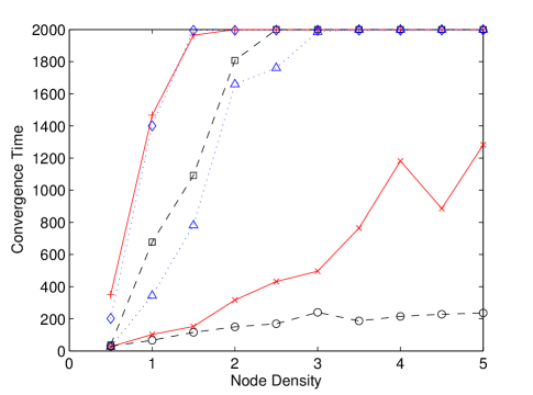
(a) Convergence time

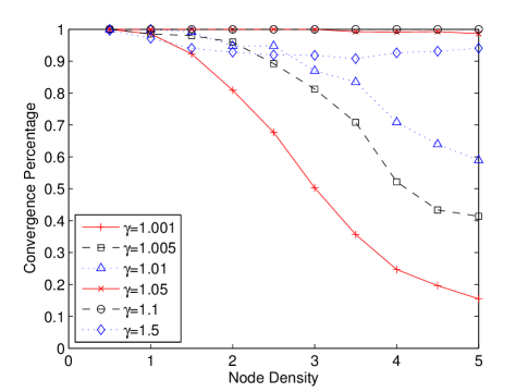
(b) Convergence percentage

Figure 8: Simulations of the multi-resolution protocol with annealing for multicast, $q=0.2$ (the same legend applies to both figures).

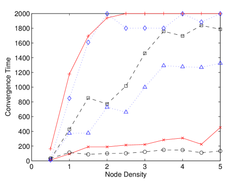
(a) Convergence time

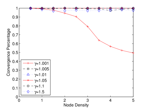
(b) Convergence percentage

Figure 9: Simulations of the multi-resolution protocol with annealing for multicast, $q=0.8$ (the same legend applies to both figures).

Figs. 8 and 9 show a simulation of Protocol 2 for a two-dimensional network. In the simulation, any one-hop peer of station $\mathbf{r}$ is an intended receiver of the multicast by station $\mathbf{r}$ with probability $q$, independent of other one-hop peers. All other simulation settings are the same as those for broadcast. Each station uses the lower bound on the resolution predicted by Theorem 6 and executes Protocol 2. Each station refines its resolutions if necessary, until the local configuration is collision-free, or the upper bound given by Theorem 6 is reached, whichever occurs first. The simulation results are similar to those for broadcast in Section IV. It appears that when $q$ is larger, the convergence time is shorter and the convergence percentage is higher. This suggests that as $q$ is larger, the lower bound given by Theorem 6 is accurate enough so fewer stations need to refine their resolutions, which helps speed up the convergence.

VI Multi-Channel Networks

In this section we assume there are $K$ orthogonal channels in the network. A station can either transmit on one channel only, or listen to all channels simultaneously at any time, i.e., stations are half-duplex. In this case, the state of a station represents both the slot $s$ and the channel $\omega$ over which the station transmits, i.e., $X_{\mathbf{r}}(t)=(\omega,s)$.

To estimate the lower and upper bounds on the resolutions for broadcast with $K$ orthogonal channels, notice that the best possible scenario in station $\mathbf{r}$’s one-hop neighborhood is that $\mathbf{r}$ occupies one slot to transmit, and in the remaining slots, $\mathbf{r}$ receives one packet on each channel; while the worst situation in station $\mathbf{r}$’s two-hop neighborhood is that every station within this two-hop neighborhood must transmit at different times. Hence we have the following results.

Theorem 8

A lower bound on the needed resolution for a collision-free configuration for broadcast with $K$ orthogonal channels to exist is given by

$$\underline{l}_{\mathbf{r}}=\biggl{\lceil}\log_{2}\biggl{(}\max_{\mathbf{r}^{\prime}\in V_{\mathbf{r}}\cup\{\mathbf{r}\}}\underline{w}_{\mathbf{r}^{\prime}}\biggr{)}\biggr{\rceil},$$ (14)

where $\underline{w}_{\mathbf{r}}=1+\frac{\lvert V_{\mathbf{r}}\rvert}{K}$. A corresponding upper bound is given by

$$\overline{l}_{\mathbf{r}}=\biggl{\lceil}\log_{2}\biggl{(}\max_{\mathbf{r}^{\prime}\in V_{\mathbf{r}}^{2}\cup\{\mathbf{r}\}}\overline{w}_{\mathbf{r}^{\prime}}\biggr{)}\biggr{\rceil},$$ (15)

where $\overline{w}_{\mathbf{r}}=1+\lvert V_{\mathbf{r}}^{2}\rvert$.

Similar arguments provide the corresponding lower and upper bounds on the resolution for multicast.

Theorem 9

A lower bound on the needed resolution for a collision-free configuration for multicast with $K$ orthogonal channels to exist is computed as follows:

$$\underline{I}_{a} = \{\mathbf{r}^{\prime}\colon M_{\mathbf{r}^{\prime}}\cap(L_{a}\cup\{a\})\neq\emptyset\},$$ (16)

$$\underline{w}_{a} = 1+\frac{\lvert\underline{I}_{a}\rvert-1}{K},$$ (17)

$$\underline{l}_{a} = \max_{a^{\prime}\in L_{a}\cup\{a\}}\underline{w}_{a^{\prime}},$$ (18)

$$\underline{l}_{\mathbf{r}} = \biggl{\lceil}\log_{2}\biggl{(}\max_{a\in M_{\mathbf{r}}}\underline{l}_{a}\biggr{)}\biggr{\rceil}.$$ (19)

A corresponding upper bound is computed as follows:

$$\overline{I}_{\mathbf{r}} = \{\mathbf{r}^{\prime}\colon M_{\mathbf{r}^{\prime}}\cap\cup_{a\in M_{\mathbf{r}}}(L_{a}^{2}\cup\{a\})\neq\emptyset\},$$ (20)

$$\overline{w}_{\mathbf{r}} = \lvert\overline{I}_{\mathbf{r}}\rvert,$$ (21)

$$\overline{l}_{\mathbf{r}} = \biggl{\lceil}\log_{2}\biggl{(}\max_{\mathbf{r}^{\prime}\in\overline{I}_{\mathbf{r}}}\overline{w}_{\mathbf{r}^{\prime}}\biggr{)}\biggr{\rceil}.$$ (22)

When there are multiple channels available, stations need to let their peers know which slot and channel they use to transmit. If a dedicated control channel (which is orthogonal to the $K$ channels for data transmission) is used to exchange state information, then $l_{\mathbf{r}}+\lceil\log_{2}K\rceil$ bits are required to represent station $\mathbf{r}$’s state: $l_{\mathbf{r}}$ bits for the slot, and $\lceil\log_{2}K\rceil$ bits for the channel. Alternatively, if there are control frames preceding each cycle, and these can be used to exchange state information on the $K$ channels for data transmission, a station can save the extra $\lceil\log_{2}K\rceil$ bits as follows: it broadcasts the state information on the $\omega$-th channel if the state information indicates a transmission on the $\omega$-th channel.

The multi-resolution protocol for broadcast on networks with multiple channels is shown as Protocol 3. The main difference from Protocol 1 is that before station $\mathbf{r}$ computes the votes using the state information from station $\mathbf{r}^{\prime}$’s one-hop neighborhood, station $\mathbf{r}$ assumes the states $(\omega,s)$ for all $\omega$ are occupied by station $\mathbf{r}^{\prime}$, where $s$ is the slot currently occupied by station $\mathbf{r}^{\prime}$ (line $3$ in Protocol 3). This is due to the half-duplex constraint: if station $\mathbf{r}^{\prime}$ transmits in slot $s$, then it cannot receive on any channel in slot $s$, meaning that packets transmitted by any one-hop peer in this slot experience collisions. The multi-resolution protocol for multicast on networks with multiple channels can be constructed similarly.

Protocol 3 Multi-Resolution MAC Protocol for Broadcast on Networks with Multiple Channels

1:  while station $\mathbf{r}$ is active do

2:        $\mathbf{r}$ sets the votes on all states to zero.

3:        for $\mathbf{r}^{\prime}\in V_{\mathbf{r}}\cup\{\mathbf{r}\}$ do

4:              Assume states $(\omega,s)$ for all $\omega$ are occupied by station $\mathbf{r}^{\prime}$, where $s$ is the slot currently occupied by $\mathbf{r}^{\prime}$.

5:              if $\mathbf{r}$ is the only station occupying its current state in station $\mathbf{r}^{\prime}$’s one-hop neighborhood then

6:                    $\mathbf{r}$’s current state is assigned a single vote of weight one.

7:              else

8:                    $\mathbf{r}$ determines which slots $s$ (according to $\mathbf{r}$’s resolution) are idle or have collisions in $\mathbf{r}^{\prime}$’s one-hop neighborhood.

9:                    A vote of weight $\frac{1}{Kn}$ is added to states $(\omega,s)$ for all $\omega$, where $n$ is the number of slots $s$ determined above.

10:              end if

11:        end for

12:        if $n_{(\omega,s)}>0$ for multiple $(\omega,s)$’s, where $n_{(\omega,s)}$ is the total weight state $(\omega,s)$ receives then

13:              Replace $n_{(\omega,s)}$ by $n_{(\omega,s)}+\epsilon$, where $\epsilon>0$, for all $(\omega,s)$.

14:        end if

15:        $\mathbf{r}$ selects state $(\omega,s)$ with a probability proportional to $f(n_{(\omega,s)})$.

16:  end while

VII Conclusion

In this paper, we have proposed multi-resolution MAC protocols for wireless networks with arbitrary topologies. We have shown that collision-free schedules can be established in a distributed manner, by allowing stations to exchange limited state information. These protocols do not require all stations to use the same resolution, i.e., the same number of states or the same length of each slot.

Future work should investigate the performance of the multi-resolution protocols under the signal-to-interference-and-noise ratio (SINR) model. This model assumes a minimum SINR requirement at a receiver for successful reception and also takes into account cumulative interference from faraway transmissions, which is more realistic. Under this model, there may be a need to reconsider what messages should be exchanged among peers in order to eliminate collisions in a distributed manner.

References

- [1] J. Lee and J. Walrand, “Design and analysis of an asynchronous zero collision MAC protocol,” 2008, arXiv:0806.3542v1 [cs.NI].
- [2] J. Barcelo, B. Bellalta, C. Cano, and M. Oliver, “Learning BEB: Avoiding collisions in WLAN,” Eunice Summer School, 2008.
- [3] M. Fang, D. Malone, K. R. Duffy, and D. J. Leith, “Decentralised learning MACs for collision-free access in WLANs,” 2010, arXiv:1009.4386v1 [cs.NI].
- [4] K. H. Hui, D. Guo, R. A. Berry, and M. Haenggi, “Performance analysis of MAC protocols in wireless line networks using statistical mechanics,” in Allerton Conference on Communication, Control and Computing, Monticello, IL, USA, Sep. 2009.
- [5] K. H. Hui, D. Guo, and R. A. Berry, “Medium access control via nearest-neighbor interactions for regular wireless networks,” in International Symposium on Information Theory, Austin, TX, USA, Jun. 2010.
- [6] L. Tassiulas and A. Ephremides, “Stability properties of constrained queueing systems and scheduling policies for maximum throughput in multihop radio networks,” IEEE Trans. Autom. Control, vol. 37, no. 12, pp. 1936–1948, Dec. 1992.
- [7] P. Chaporkar, K. Kar, X. Luo, and S. Sarkar, “Throughput and fairness guarantees through maximal scheduling in wireless networks,” IEEE Trans. Inf. Theory, vol. 54, no. 2, pp. 572–594, Feb. 2008.
- [8] X. Lin and N. B. Shroff, “The impact of imperfect scheduling on cross-layer rate control in wireless networks,” in 24th Annual Joint Conference of the IEEE Computer and Communications Societies (INFOCOM ’05), Miami, FL, USA, Mar. 2005, pp. 1804–1814.
- [9] G. Sharma, N. B. Shroff, and R. R. Mazumdar, “Joint congestion control and distributed scheduling for throughput guarantees in wireless networks,” in 26th Annual Joint Conference of the IEEE Computer and Communications Societies (INFOCOM ’07), Anchorage, AK, USA, May 2007, pp. 2072–2080.
- [10] E. Modiano, D. Shah, and G. Zussman, “Maximizing throughput in wireless networks via gossiping,” in ACM SIGMETRICS, Saint Malo, France, Jun. 2006, pp. 27–38.
- [11] A. Eryilmaz, A. Ozdaglar, and E. Modiano, “Polynomial complexity algorithms for full utilization of multi-hop wireless networks,” in 26th Annual Joint Conference of the IEEE Computer and Communications Societies (INFOCOM ’07), Anchorage, AK, USA, May 2007, pp. 499–507.
- [12] X. Lin and S. B. Rasool, “Constant-time distributed scheduling policies for ad hoc wireless networks,” IEEE Trans. Autom. Control, vol. 54, no. 2, pp. 231–242, Feb. 2009.
- [13] Y. Yi, G. de Veciana, and S. Shakkottai, “MAC scheduling with low overheads by learning neighborhood contention patterns,” IEEE/ACM Trans. Netw., vol. 18, no. 5, pp. 1637–1650, Oct. 2010.
- [14] I. Rhee, A. Warrier, M. Aia, J. Min, and M. L. Sichitiu, “Z-MAC: A hybrid MAC for wireless sensor networks,” IEEE/ACM Trans. Netw., vol. 16, no. 3, pp. 511–524, Jun. 2008.
- [15] A. Ephremides and T. V. Truong, “Scheduling broadcasts in multihop radio networks,” IEEE Trans. Commun., vol. 38, no. 4, pp. 456–460, Apr. 1990.
- [16] R. Ramaswami and K. K. Parhi, “Distributed scheduling of broadcasts in a radio network,” in 8th Annual Joint Conference of the IEEE Computer and Communications Societies (INFOCOM ’89), Ottawa, Ontario, Canada, Apr. 1989, pp. 497–504.
- [17] D. Guo and L. Zhang, “Virtual full-duplex wireless communication via rapid on-off-division duplex,” in Allerton Conference on Communication, Control and Computing, Monticello, IL, USA, Sep. 2010.
- [18] L. Zhang and D. Guo, “Wireless peer-to-peer mutual broadcast via sparse recovery,” in International Symposium on Information Theory, Saint Petersburg, Russia, Jul./Aug. 2011.
- [19] X. Guyon and C. Hardouin, “Markov chain markov field dynamics: Models and statistics,” Statistics, vol. 36, no. 4, pp. 339–363, 2002.
- [20] N. Wen and R. A. Berry, “Location-based MAC protocols for mobile wireless networks,” in 2007 Information Theory and Applications Workshop (ITA), San Diego, CA, USA, 2007.
- [21] D. R. Fulkerson and O. A. Gross, “Incidence matrices and interval graphs,” Pacific Journal of Mathematics, vol. 15, no. 3, pp. 835–855, 1965.
- [22] D. J. Leith and P. Clifford, “A self-managed distributed channel selection algorithm for WLANs,” in 4th International Symposium on Modeling and Optimization in Mobile, Ad Hoc and Wireless Networks, 2006 (WiOpt 2006), Apr. 2006, pp. 1–9.