Cosmology today–A brief review

Abstract

This is a brief review of the standard model of cosmology. We first introduce the FRW models and their flat solutions for energy fluids playing an important role in the dynamics at different epochs. We then introduce different cosmological lengths and some of their applications. The later part is dedicated to the physical processes and concepts necessary to understand the early and very early Universe and observations of it.

1 Introduction

The purpose of the present review is to provide the reader with an outline of modern cosmology. This science is passing through a revolutionary era, mainly because recent high precision observations have severely constrained theoretical speculations, and opened new windows to the cosmos. Tracking the recent history, in the late 1940’s George Gamow Ga46 predicted that the Universe should had begun from a very dense state, characterized by a huge density at very high temperatures, a scenario dubbed the Big Bang, that was conjectured by George Lemaître in the early 30’s. This scenario predicts that matter and light were at very high energetic states, and both components behaved as a radiation fluid, in thermal equilibrium described as Planck blackbody (Bose-Einstein and the related Fermi-Dirac distributions). This initial state remains today imprinted in the Cosmic Microwave Background Radiation (CMBR). Gamow’s scenario predicted this primeval radiation would be measured at a temperature of only few Kelvin’s degrees; since the expansion of the Universe cools down any density component. Robert Dicke, and others, begun the race to discover this radiation coming from the cosmos, and in 1965 A. A. Penzias and R.W. Wilson of the Bell telephone laboratories discovered, by chance, this radiation form, confirming the general Big Bang scenario; see the original references published in Ref. KoTu88 .

During this elapsed period the Big Bang scenario was generally accepted. However, some key questions remained open, for instance, whether or not this radiation was of Planckian nature to entirely confirm that the Universe was in thermal equilibrium at the very beginning of time. In 1990 a modern version of the Penzias–Wilson experiment was carried out. This experiment, lead by G. Smoot and J. Mather with the Cosmic Background Explorer (COBE) satellite, started a new high precision experimental era in cosmology Mather90 . The COBE team for the first time revealed that the Universe was in equilibrium (the radiation had the Planck form to high precision), and was almost homogeneous and isotropic, but not completelySm92 . The tiny ($10^{-5}$) anisotropies found by COBE –also imprinted in the matter distribution– were lately the responsible for the formation of stars, galaxies, clusters, and all large scale structures of our Universe.

The origin of these tiny anisotropies is presumably in quantum fluctuations of fundamental fields of nature which were present in the very early Universe. Modern quantum field theories, together with cosmological models, help to understand how this small fluctuations evolved to become of cosmic scales, enabling COBE to detect them. This satellite and other more recent cosmological probes, such as BOOMERANG, MAXIMA, WMAP and now PLANCK satellite that measured CMBR and the Two degree Field (2dF) galaxy survey and the Sloan Digital Sky Survey (SDSS), among others, not only confirmed with a great accuracy some of the theoretical predictions of the standard big bang cosmological model, but also opened the possibility to test theories and scenarios applicable in very early Universe, such as inflation, or in present times, such as quintessence. In this way, cosmology that used to be a purely theoretical and often speculative science, is today subject to high precision tests in light of these new observations BrCeSa04 ; AmTs10 .

2 On the standard model of cosmology

We begin our study by reviewing some aspects of the standard lore of physical and theoretical cosmology. In doing that we consider the Friedmann-Robertson-Walker (FRW) model in Einstein’s general relativity (GR) theory. We shall make use of “natural” units $\hbar=c=k_{B}=1$ and our geometrical sign conventions are as in Ref. MiThWh73 .

2.1 FRW models

The cosmological principle states that the Universe is both spatially homogeneous and isotropic on the large scale, which was originally assumed but now observed to be valid for the very large large scale of the Universe. This homogeneous and isotropic space–time symmetry was originally studied by Friedmann, Robertson, and Walker (FRW), see Refs. Fr22Ro35Wa36 . The symmetry is encoded in and defines the unique form of the line element:

$$ds^{2}=-dt^{2}+a^{2}(t)\,\ \left[\frac{dr^{2}}{1-kr^{2}}+r^{2}(d\theta^{2}+{\rm sin}^{2}\theta\,d\phi^{2})\right],$$ (1)

where $t$ is the cosmic time, $r-\theta-\phi$ are polar coordinates, which can be adjusted so that the constant curvature takes the values $k$ = 0, +1, or $-1$ for a flat, closed, or open space, respectively. $a(t)$ is the unknown potential of the metric that encodes the size at large scales, more formally is the scale factor of the Universe.

To then solve this line element for the scale factor of the Universe $a(t)$ and perturbations one simply needs a valid theory of gravity. The standard model of cosmology is based on GR, which can be derived from the Einstein-Hilbert Lagrangian

$${\cal L}=\frac{1}{16\pi G}(R+L_{m})\sqrt{-g}\,\ ,$$ (2)

where $R$ is the Ricci scalar, $G$ the Newton constant, and $g=|g_{\mu\nu}|$ the determinant of the metric tensor. By performing the metric variation of this equation, one obtains the well known Einstein’s field equations

$$R_{\mu\nu}-\frac{1}{2}Rg_{\mu\nu}=8\pi GT_{\mu\nu}\,\ ,$$ (3)

where $T_{\mu\nu}\equiv-\frac{2}{\sqrt{-g}}\frac{\partial L_{m}\sqrt{-g}}{\partial g^{\mu\nu}}$ is the stress energy–momentum tensor, which is a symmetric tensor. Thus, Eq. (3) is a collection of ten coupled partial differential equations. However, the theory is diffeomorphism invariant, and one adds to them a gauge condition, implying in general four extra equations to Eq. (3) that reduce the degrees of freedom.

The beautifully symmetric FRW solutions to the Einstein Eqs. (3) represent a cornerstone in the development of modern cosmology, since with them it is possible to understand the expansion of Universe as was realized in the 1920’s through Hubble’s law of expansion Hu27 . With this FRW metric, the GR cosmological field equations are,

$$H^{2}\equiv\left(\frac{\dot{a}}{a}\right)^{\!2}=\frac{8\pi G}{3}\rho-\frac{k}{a^{2}}$$ (4)

and

$$\frac{\ddot{a}}{a}=-\frac{4\pi G}{3}(\rho+3p)\,\ ,$$ (5)

where $H$ is the Hubble parameter; $\rho$ and $p$ are the density and pressure of the perfect fluid considered, that is, $T_{\mu\nu}=\rho u_{\mu}u_{\nu}+p(u_{\mu}u_{\nu}+g_{\mu\nu})$, where $u_{\mu}=\delta^{0}_{\mu}$ is the fluid’s four velocity in comoving coordinates. Dots stand for cosmic time derivatives.

Assuming energy–momentum tensor conservation, $T_{\mu\,\ ;\nu}^{~{}\nu}=0$, is valid, one obtains the continuity equation,

$$\dot{\rho}+3H(\rho+p)=0\,\ .$$ (6)

The above system of equations (4), (5), and (6) implies three unknown variables ($a$, $\rho$, $p$) for three equations, but the equations are not all linearly independent, just two of them. Thus, an extra assumption has to be made to close the system. The answer should come from the micro-physics of the fluids considered. For the moment let us assume a barotropic equation of state that is characteristic for different cosmic fluids, $w={\rm const.}$,

$$\frac{p}{\rho}=w=\left\{\begin{array}[]{l@{\quad{\rm for} \quad}l}\frac{1}{3}&{\rm radiation~{}or~{}relativistic~{}matter}\\ 0&{\rm dust}\\ 1&{\rm stiff~{}fluid}\\ -1&{\rm cosmological~{}constant}\end{array}\right.$$ (7)

to integrate Eq. (6), yielding

$$\rho=\frac{M_{w}}{a^{3(1+w)}}~{}~{}~{}~{}~{}~{}~{}{\rm or}~{}~{}~{}~{}~{}~{}\frac{\rho_{x}}{\rho_{x~{}0}}=\left(\frac{a_{0}}{a}\right)^{3(1+w)}\,\ ,$$ (8)

where $M_{w}$ is the integration constant and is different dimensioned by considering different $w-$fluids. With this equation the system is closed and can be solved once the initial conditions are known.

In addition to the above fluids, one can include an explicit cosmological constant ($\Lambda$) in Eq. (4) and arrange it in the following form:

$$\Omega\equiv\Omega_{R}+\Omega_{M}+\Omega_{\Lambda}=1+\frac{k}{a^{2}H^{2}}$$ (9)

with $\Omega_{R}$ being the radiation component dominated by the CMB and small ($5\times 10^{-5}$ at present), $\Omega_{M}\equiv\frac{8\pi G\rho_{m}}{3H^{2}}$ and $\Omega_{\Lambda}\equiv\frac{\Lambda}{3H^{2}}$. The parameter $\Omega$ is called the density parameter, which is composed of a matter part and a cosmological constant term. Thus, we see that the different values of the density parameters $(\Omega_{m},\Omega_{\Lambda})$ will impose different values for the curvature term. If $\Omega>1$, it turns out $k$ is greater than zero, signifying a Universe with a positive curvature (closed Universe). If $\Omega<1$, then $k<0$, this corresponds to a negative curvature (open Universe). A critical value is obtained obviously when $\Omega=1$, then the spatial curvature is null, $k=0$. The value of the energy density for which $\Omega=[\rho+\Lambda/(8\pi G)]/\rho_{c}=1$ holds is known as the critical density, $\rho_{c}\equiv 3H^{2}/8\pi G$. The last term in Eq. (9) can be defined as $\Omega_{k}=-\frac{k}{a^{2}H^{2}}$ and thus the Friedman equation becomes a constriction for the density parameters $\sum_{i}\Omega_{i}=1$, and this expression holds at any time. It is useful to define an alternative measure of the expansion of the Universe through the redshift ($z$), $1+z\equiv a_{0}/a(t)$, where $a_{0}$ is the scale factor at present and is the set to unity by convention. Today $z_{0}=0$ and in the early Universe the redshift grows. In terms of the redshift the density parameters are, from Eq. (8), $\Omega_{i}=\Omega_{i}^{(0)}(1+z)^{3(1+w)}$; quantities with a subindex or superindex “0” are evaluated at the present time.

Let us very briefly recall which $w-$values are needed to describe the different epochs of the Universe’s evolution. The assumption that $w=1/3$ is valid for a “fluid” of radiation and/or of ultra-relativistic matter ($T\gg m$, $m$ being its rest mass). This epoch is of importance at the beginning of the hot big bang theory, where the material content of the Universe consisted of photons, neutrinos, electrons, and other massive particles with very high kinetic energy. After some Universe cooling, some massive particles decayed and others survived (protons, neutrons, electrons) whose masses eventually dominated over the radiation components (photon, neutrinos) at the equality epoch ($\rho_{\rm rel}=\rho_{m}$) at $z_{\rm eq}\sim 3200$ wmap7 . From this epoch and until recent efolds of expansion ($z_{\rm DE}\sim 1/2$) the main matter component produced effectively no pressure on the expansion and, therefore, one can accept a model filled with dust, $w=0$, to be representative for the energy content of the Universe in the interval $3200<z<1/2$. The dust equation of state is then representative of inert, cold dark matter (CDM). Dark matter (DM) does not (significantly) emit light and therefore it is dark. Another possibility is that dark matter interacts weakly and is generically called WIMP (Weakly Interacting Massive Particle), being the neutralino the most popular WIMP candidate. Another popular dark matter candidate is the axion, a hypothetical particle postulated to explain the conservation of the CP symmetry in quantum chromodynamics (QCD). Back to the Universe evolution, from $z\sim 1/2$ and until now the Universe happens to be accelerating with an equation of state $w\approx-1$, due to some constant energy that induces a cosmological constant, $\Lambda=8\pi G\rho=$const. The cosmological constant is the generic factor of an inflationary solution, see the $k=0$ solution below, Eq. (15). The details of the expansion are still unknown and it is possible that the expansion is due to some new fundamental field (e.g. quintessence) that induces an effective $\Lambda(t)\sim$const. One calls (M. Turner dubbed it) dark energy (DE) to this new element. Dark energy does not emit light nor any other particle, as so far known, it simply behaves as a (transparent) media that gravitates with an effective negative pressure. The physics behind dark energy or even the cosmological constant is unclear since theories of grand unification (or theories of everything, including gravity) generically predict a vacuum energy associated with fundamental fields, $<0|T_{\mu\nu}|0>=<\rho>g_{\mu\nu}$, that turns out to be very large. This can be seen by summing the zero-point energies of all normal modes of some field of mass $m$, to obtain $<\rho>\approx M^{4}/(16\pi^{2})$, where $M$ represents some cutoff in the integration, $M\gg m$. Then, assuming GR is valid up to the Planck ($Pl$) scale, one should take $M\approx 1/\sqrt{8\pi G}$, which gives $<\rho>=10^{71}$ GeV⁴. This term plays the role of an effective cosmological constant of $\Lambda=8\pi G<\rho>\approx M_{Pl}^{2}\sim 10^{38}$ GeV² which must be added to the Einstein equations (3) and yields an inflationary solution Eq. (15). However, since the cosmological constant seems to dominate the Universe dynamics nowadays, one has that

$$\Lambda\approx 8\pi G\rho_{0}=3H_{0}^{2}\sim 10^{-83}{\rm GeV}{}^{2}.$$ (10)

which is very small compared with the above value derived on dimensional grounds. Thus, the cosmological constraint and theoretical expectations are rather dissimilar, by about 121 orders of magnitude! Even if one considers symmetries at lower energy scales the theoretical $\Lambda$ is indeed smaller, but never as small as the cosmological constraint: $\Lambda_{GUT}\sim 10^{21}$ GeV², $\Lambda_{SU(2)}\sim 10^{-29}$ GeV². This problem has been reviewed since decades ago We89 ; CaPrTu92 and remains open.

The ordinary differential equations system described above needs a set of initial, or alternatively boundary, conditions to be integrated. One has to assume a set of two initial values, say, $(\rho(t_{*}),\dot{a}(t_{*}))\equiv(\rho_{*},\dot{a}_{*})$ at some (initial) time $t_{*}$, in order to determine its evolution. The full analysis of it can be found in many textbooks We72 ; MiThWh73 . Here, in order to show some physical, early Universe consequences we assume $k=0$, justified as follows: From Eqs. (4) and (8) one notes that the expansion rate, given by the Hubble parameter, is dominated by the density term as $a(t)\rightarrow 0$, since $\rho\sim 1/a^{3(1+w)}>k/a^{2}$ for $w>-1/3$, that is, the flat solution is very well fitted at the very beginning of times. Therefore, assuming $k=0$, Eq. (4) implies

$$a(t) = [6\pi GM_{w}(1+w)^{2}]^{\frac{1}{3(1+w)}}(t-t_{*})^{\frac{2}{3(1+w)}}$$ (14)

$$= \left\{\begin{array}[]{l@{\quad{\rm for} \quad}l}(\frac{32}{3}\pi GM_{\frac{1}{3}})^{1/4}~{}(t-t_{*})^{1/2}&w=\frac{1}{3}~{}{\rm radiation}\\ (6\pi GM_{0})^{1/3}~{}~{}~{}(t-t_{*})^{2/3}&w=0~{}{\rm dust}\\ (24\pi GM_{1})^{1/6}~{}~{}(t-t_{*})^{1/3}&w=1~{}{\rm stiff~{}fluid}\\ \end{array}\right.$$

and

$$a(t)=a_{*}e^{Ht}\qquad{\rm for}\qquad w=-1~{}{\rm cosmological~{}constant}$$ (15)

where the letters with a subindex “$*$” are integration constants, representing quantities evaluated at the beginning of times, $t=t_{*}$. To obtain Eq. (15), the argument given right above to neglect $k$ is not anymore valid, since here $\rho={\rm const.}$; that is, from the very beginning it must be warranted that $H^{2}\approx\frac{8\pi G}{3}\rho_{*}>k/a^{2}_{*}$, otherwise $k$ cannot be ignored. Nevertheless if $\Lambda$ is present, it will eventually dominate over the other decaying components, this is the so called cosmological no-hair theorem ChMo94 . A general feature of all the above solutions is that they are expanding, at different Hubble rates, $H=\frac{2}{3(1+w)}\frac{1}{t}$ for Eqs. (14) and $H=$const. for Eq. (15).

From Eq. (14) one can immediately see that at $t=t_{*},\,\ a_{*}=0$ and from Eq. (8), $\rho_{*}=\infty$, that is, the solution has a singularity at that time, at the Universe’s beginning; this initial cosmological singularity is precisely the big bang singularity. As the Universe evolves the Hubble parameter goes as $H\sim 1/t$, i.e., the expansion rate decreases; whereas the matter-energy content acts as an expanding agent, cf. Eq. (4), it decelerates the expansion, however, asymptotically decreasing, cf. Eqs. (5) and (8). In that way, $H^{-1}$ represents an upper limit to the age of the Universe; for instance, $H^{-1}=2t$ for $w=1/3$ and $H^{-1}=3t/2$ for $w=0$, $t$ being the Universe’s age.

The exponential expansion (15) possesses no singularity (at finite times), being the Hubble parameter a constant. A fundamental ingredient of this inflation is that the right hand side of Eq. (5) is positive, $\ddot{a}>0$, and this is performed when $\rho+3p<0$, that is, one does not have necessarily to impose the stronger condition $w=-1$, but it suffices that $w<-1/3$, in order to have a moderate inflationary solution; for example, $w=-2/3$ it implies $a=a_{*}t^{2}$, a mild power-law inflation.

Since the scale factor evolves as a smooth function of time (most of the time!), one is able to use it as a variable, instead of time, in such as a way that $d/dt=a\,H\,d/da$. This change of variable helps to integrate the continuity equation for non-constant $w(a)$ to obtain:

$$\rho(a)=\rho_{0}e^{-3\int[1+w(a)]da/a}.$$ (16)

If, for instance, one parametrizes dark energy through an analytic function of the scale factor, $w(a)$, one immediately obtains its solution in terms of

$$t=\int\frac{1}{\sqrt{8\pi G\rho(a)/3}}\frac{da}{a}.$$ (17)

In cosmology, typical times and distances are determined mainly by the Hubble parameter, and in practice measurements are often related to redshift, as measured from stars, gas, etc. It is then useful to express the Friedmann Eq. (4) in terms of the redshift. The standard model of cosmology considers a Universe filled baryons, photons, neutrinos, CDM, and a cosmological constant ($\Lambda$), and is termed $\Lambda$CDM for short. For this model one obtains:

$$H^{2}=H_{0}^{2}\sum_{i}\Omega_{i}^{(0)}(1+z)^{3(1+w_{i})},$$ (18)

where $w_{i}$ is the equation of state parameter for each of the fluids considered. The present contribution of the main energy components can be fitted from different cosmological probes, obtaining $\Omega_{b}^{(0)}=0.046\pm 0.002$, $\Omega_{\rm DM}^{(0)}=0.23\pm 0.01$, and $\Omega_{\Lambda}^{(0)}=0.73\pm 0.02$, together with a Hubble constant of $70.4^{+1.3}_{-1.4}$ km/s/Mpc wmap7 . Around $96\%$ of mater-energy the Universe is composed of dark components!

In general, if dark energy is a function of the redshift, from Eq. (16) one can generalize the above equation to:

$$H(z)^{2}/H_{0}^{2}=\Omega_{m}^{(0)}(1+z)^{3}+\Omega_{\gamma}^{(0)}(1+z)^{4}+\Omega_{k}^{(0)}(1+z)^{2}+\Omega_{DE}^{(0)}{\sf f}(z)\,,$$ (19)

where $m$ stands for dark matter and baryons, $\gamma$ for photons, and

$${\sf f}(z)={\rm exp}\left[3\int_{0}^{z}\frac{1+w(z^{\prime})}{1+z^{\prime}}dz^{\prime}\right]\,.$$ (20)

Eq. (17) gives the age of the Universe in terms of the redshift, $H_{0}$, and the density parameters:

$$t_{0}=H_{0}^{-1}\int_{0}^{\infty}\frac{dz}{(1+z)H(z)}.$$ (21)

When combining different cosmological probes one obtains for the $\Lambda$CDM model an age of $t_{0}=13.75\pm 0.11$ Gyr wmap7 .

2.2 Cosmic distances and their measurements

It is useful to write the FRW metric, Eq. (1), in terms of a new distance coordinate ($\chi$)

$$ds^{2}=-dt^{2}+a^{2}(t)\left[d\chi^{2}+f_{k}^{2}(\chi)(d\theta^{2}+\sin^{2}\theta\,d\phi^{2})\right]\,,$$ (22)

where

$$f_{k}(\chi)=\left\{\begin{array}[]{lll}{\rm sin}\chi\,,&k=+1\,,\\ \chi\,,&k=0\,,\\ {\rm sinh}\chi\,,&k=-1\,.\end{array}\right.$$ (26)

Now we proceed to define some cosmic distances necessary to understand the cosmic physics.

Causal horizon. The region of space that can be connected to some other region by causal physical processes, at most through the propagation of light, implies $ds^{2}=0$. For the FRW Eq. (1) or (22), in spherical coordinates with $\theta,\phi=$const. implies that Ri56 ; We72 :

$$\chi_{H}=\int^{\chi_{H}}_{0}d\chi=\int^{t_{0}}_{t}\frac{dt^{\prime}}{a(t^{\prime})}=\frac{1}{a_{0}H_{0}}\int^{z}_{0}\frac{dz^{\prime}}{E(z^{\prime})}$$ (27)

this is the so-called comoving distance, being the distance between two points in the Universe in which the expansion is factored out. Now, the causal or particle horizon, $d_{H}$ is given by:

$$d_{H}(t)=a(t)\,\int^{\chi_{H}}_{0}d\chi=a(t)\,\int^{t}_{t_{*}}\frac{dt^{\prime}}{a(t^{\prime})}.$$ (28)

In order to analyze the whole horizon evolution, from nowadays ($t_{0}$) to the Planck time ($t_{Pl}$), we have to consider all the Universe stages, but for brevity we shall not include the current accelerated expansion. We firstly compute the horizon for the matter dominated era $t_{\rm eq.}\leq t\leq t_{0}$ and secondly for the radiation era $t\leq t_{\rm eq.}$, because they are differently determined by Eq. (14), where we set $t_{*}=0$ for convenience. For the matter epoch one has $a(t)=a_{0}(t/t_{0})^{2/3}$, then the first equation above gives $\chi_{H}=\frac{3}{a_{0}}(t_{0}^{2}~{}t)^{1/3}$; from the second equation one obtains the horizon $d_{H}(t)=3t=2H^{-1}$. For the radiation period, one has that $\chi_{H}=\frac{2}{a_{\rm eq.}}(t_{\rm eq.}~{}t)^{1/2}$ and $d_{H}(t)=2t=H^{-1}$. We see, for the matter dominated era, the causal horizon is twice the Hubble distance, $H^{-1}$ (sometimes called Hubble horizon), and they are equal to each other during the radiation dominated era; therefore, one uses them interchangeably. It is clearly seen for both eras that as $t\rightarrow 0$, the Universe is causally disconnected, being $a(t)>d_{H}(t)$. But, on the other side, by that time the CMBR was already highly isotropic and with a black body spectrum. Then, one has to take for granted that the initial conditions for all small horizon volumes were very fine tuned to account for the present observed large angle CMBR levels of isotropy, with $\delta T/T\approx{\rm few}\times 10^{-5}$. This is the horizon problem.

Event Horizon. The event horizon, $d_{e}$, determines the region of space which will keep in causal contact after some time; that is, it delimits the region from which one can ever receive (up to some time $t_{\rm max}$) information about events taking place now (at the time $t$):

$$d_{e}(t)=a(t)\int_{t}^{t_{\rm max}}\frac{dt^{\prime}}{a(t^{\prime})}\,\ .$$ (29)

For a flat model during its matter dominated era ($a\sim t^{2/3}$), $d_{e}\rightarrow\infty$ as $t_{\rm max}\rightarrow\infty$.

Luminosity distance. The luminosity distance is the distance measured using the energy flux (${\cal F}$) observed by a light source with absolute luminosity ($L_{s}$):

$$d_{L}^{2}\equiv\frac{L_{s}}{4\pi{\cal F}}\,,$$ (30)

where ${\cal F}=L_{0}/S$, being $L_{0}$ the observed luminosity and $S=4\pi(a_{0}f_{k}(\chi))^{2}$ is the sphere area at $z=0$. The luminosity distance becomes

$$d_{L}^{2}=(a_{0}f_{k}(\chi))^{2}\frac{L_{s}}{L_{0}}\,.$$ (31)

If we express the energy emitted by a light pulse in a time interval $\Delta t_{1}$ as $\Delta E_{1}$, the absolute luminosity is given by $L_{s}=\Delta E_{1}/\Delta t_{1}$. Similarly we define $L_{0}=\Delta E_{0}/\Delta t_{0}$, where $\Delta E_{0}$ is the detected energy in a time $\Delta t_{0}$. On the other hand, since the photon energy can be expressed in terms of its wavelenght ($\lambda$), one has that $\Delta E_{1}/\Delta E_{0}=\lambda_{0}/\lambda_{1}=1+z$ and moreover $c=1$, being constant implies that $\lambda_{1}/\Delta t_{1}=\lambda_{0}/\Delta t_{0}$, from which we finally have that

$$\frac{L_{s}}{L_{0}}=\frac{\Delta E_{1}}{\Delta E_{0}}\frac{\Delta t_{0}}{\Delta t_{1}}=(1+z)^{2},$$ (32)

and the luminosity distance becomes

$$d_{L}=a_{0}f_{k}(\chi)(1+z).$$ (33)

Since $f_{k}(\chi)$ depends on $\chi$ and this on the redshift, cf. Eq. (27), thus by measuring the luminosity distance, we can determine the expansion rate of the Universe. For the $\Lambda$CDM model one finds that CoSaTs06

$$d_{L}=\frac{(1+z)}{H_{0}}\int_{0}^{z}\frac{dz^{\prime}}{\sqrt{\sum_{i}\Omega_{i}^{0}(1+z^{\prime})^{3(1+w)}}}.$$ (34)

The luminosity distance becomes larger when the cosmological constant is present and this is what was found to fit better the supernovae Ia.

In practice, one uses the relationship of the apparent ($m$) and absolute ($M$) magnitude, related to the luminosity measured at present and when emitted, respectively to have:

$$m-M=5\,{\rm Log}_{10}\left(\frac{d_{L}}{\rm Mpc}\right)+25.$$ (35)

By adjusting best fit curves to their data, two different supernova groups Ri99-Pe99 found a clear evidence for $\Lambda$ in the late 90’s. The presence of a cosmological constant makes the Universe not only expanding, but accelerating and, in addition, its age is older, not conflicting with globular cluster ages. With the course of the years, various supernova groups have been getting more confidence that the data is compatible with the presence of dark energy, dark matter, and a high value of Hubble parameter. One of the latest data release, the Union2 compilation Am10 , reports that the flat concordance $\Lambda$CDM model remains an excellent fit to the data with the best fit constant equation of state parameter $w=-0.997^{+0.050}_{-0.054}$ for a flat Universe, and $w=-1.035^{+0.055}_{-0.059}$ with curvature. Also, they found that $\Omega_{m}=0.270\pm 0.021$ (including baryons and DM) for fixed $\Omega_{k}=0$. That is, $\Omega_{\Lambda}=0.730\pm 0.021$.

Angular diameter distance. The angular diameter distance is given by

$$d_{A}\equiv\frac{\Delta x}{\Delta\theta},$$ (36)

where $\Delta\theta$ is the angular aperture of an object of size $\Delta x$ orthogonal to the line of sight in the sky. Usually this distance is used in the CMBR anisotropy observations, since the source emitting the radiation is on a surface of a sphere of radius $\chi$ with the observer located at the center; it is also used in the determination of the BAO feature, see below. Thus, the size $\Delta x$ at the time $t_{1}$ in the Friedmann metric, Eq. (22), is given by

$$\Delta x=a(t_{1})f_{k}(\chi)\Delta\theta.$$ (37)

Thus, the angular diameter distance is

$$d_{A}=a(t_{1})f_{k}(\chi)=\frac{a_{0}f_{k}(\chi)}{1+z}$$ (38)

and comparing it with Eq. (33) one has

$$d_{A}=\frac{d_{L}}{(1+z)^{2}},$$ (39)

which is called duality relationship. Eq. (39) is valid beyond the FRW metric. In fact, it is valid for any metric in which the flux is conserved.

3 The physical Universe

In the following we provide with theoretical tools to understand the physics of the early Universe. We treat some micro-physics that rules the interactions of the particles and fields.

3.1 Thermodynamics in the early Universe

In the early Universe one considers a plasma of particles and their antiparticles, as originally was done by Gamow Ga46 , who has first considered a physical scenario for the hot big bang model for the Universe’s beginning. Later on, with the development of modern particle physics theories in the 70’s it was unavoidable to think about a physical scenario which should include the “new” physics for the early Universe. It was also realized that the physics described by GR should not be applied beyond Planckian initial conditions, because there the quantum corrections to the metric tensor become very important, a theory which is still in progress. So the things, one assumes at some early time, $t\,{}^{>}_{\sim}\,t_{Pl}$, that the Universe was filled with a plasma of relativistic particles which include quarks, leptons, and gauge and Higgs bosons, all in thermal equilibrium at a very high temperature, $T$, with some gauge symmetry dictated by a particle physics theory.

Theoretically, in order to work in that direction one introduces some thermodynamic considerations necessary for the description of the physical content of the Universe, which we would like to present here. Assuming an ideal-gas approximation, the number density $n_{i}$ of the particles of type $i$, with a momentum $q$, is given by a Fermi or Bose distribution KoTu90 :

$$n_{i}=\frac{g_{i}}{2\pi^{2}}\int\frac{q^{2}dq}{e^{(E_{i}-\mu_{i})/T}\pm 1}\,\ ,$$ (40)

where $E_{i}=\sqrt{m_{i}^{2}+q^{2}}$ is the particle energy, $\mu_{i}$ is the chemical potential, the sign $(+)$ applies for fermions and $(-)$ for bosons, and $g_{i}$ is the number of spin states. One has that $g_{i}=2$ for photons, quarks, baryons, electron, muon, tau, and their antiparticles, but $g_{i}=1$ for neutrinos because they are only left-handed. For the particles existing in the early Universe one usually assumes that $\mu_{i}=0$: one expects that in any particle reaction the $\mu_{i}$ are conserved, just as the charge, energy, spin, and lepton and baryon number, as well. For photons, which can be created and/or annihilated after some particle’s collisions, its number density, $n_{\gamma}$, must not be conserved and its distribution with $\mu_{\gamma}=0,\,\ E=q=\hbar\omega$, reduces to the Planckian one. For other constituents, in order to determine the $\mu_{i}$, one needs $n_{i}$; one notes from Eq. (40) that for large $\mu_{i}>0,\,\ n_{i}$ is large too. One does not know $n_{i}$, but the WMAP data constrains the baryon density at nucleosynthesis such that CyFiOlSk04 :

$$\eta\equiv\frac{n_{B}}{n_{\gamma}}\equiv\frac{n_{\rm baryons}-n_{\rm anti-baryons}}{n_{\gamma}}=6.14\pm 0.25\times 10^{-10}\,\ .$$ (41)

The smallness of the baryon number density, $n_{B}$, relative to the photon’s, suggests that $n_{\rm leptons}$ may also be small compared with $n_{\gamma}$. Therefore, one takes for granted that $\mu_{i}=0$ for all particles. Why the ratio $n_{B}/n_{\gamma}$ is so small, but not zero, is one of the puzzles of the standard model of cosmology called baryogenesis, as we will explain below.

The above approximation allows one to treat the density and pressure of all particles as a function of the temperature only. According to the second law of thermodynamics, one has We72 : $dS(V,T)=\frac{1}{T}[d(\rho V)+pdV]$, where $S$ is the entropy in a volume $V\sim a^{3}(t)$ with $\rho=\rho(T),\,\ p=p(T)$ in equilibrium. Furthermore, the following integrability condition $\frac{\partial^{2}S}{\partial T\partial V}=\frac{\partial^{2}S}{\partial V\partial T}$ is also valid, which turns out to be

$$\frac{dp}{dT}=\frac{\rho+p}{T}\,\ .$$ (42)

On the other hand, the energy conservation law, Eq. (6), leads to

$$a^{3}(t)\frac{dp}{dt}=\frac{d}{dt}[a^{3}(t)(\rho+p)]$$ (43)

and using Eq. (42), the latter takes the form $\frac{d}{dt}[\frac{a^{3}(t)}{T}(\rho+p)]=0$, and using Eq. (42) again, the entropy equation can be written as $dS(V,T)=\frac{1}{T}d[(\rho+p)V]-\frac{V}{T^{2}}(\rho+p)dT$. Last two equations imply that the entropy is a constant of motion:

$$S=\frac{a^{3}}{T}[\rho+p]={\rm const.}\,.$$ (44)

The density and pressure are given by

$$\rho\equiv\int E_{i}n_{i}dq\,\ ,\qquad p\equiv\int\frac{q^{2}}{3E_{i}}n_{i}dq\,\ .$$ (45)

For photons or ultra-relativistic fluids, $E=q$, these equations become such that $p=\frac{1}{3}\rho$, and then confirming Eq. (7) with $w=1/3$, and after integrating Eq. (42), it comes out that

$$\rho=bT^{4}\,,$$ (46)

with the constant of integration, $b$. In a real scenario there are many relativistic particles present, each of which contributes like Eq. (46). By including all of them, $\rho=\sum_{i}\rho_{i}$ and $p=\sum_{i}p_{i}$ over all relativistic species, one has that $b(T)=\frac{\pi^{2}}{30}(N_{B}+\frac{7}{8}N_{F})$, which depends on the effective relativistic degrees of freedom of bosons ($N_{B}$) and fermions ($N_{F}$); therefore, this quantity varies with the temperature; different $i-$species remain relativistic until some characteristic temperature $T\approx m_{i}$, after that the value $N_{F_{i}}$ (or $N_{B_{i}}$) contributes no more to $b(T)$. The factor 7/8 accounts for the different statistics the particles have, see Eq. (40). In the standard model of particles physics $b\approx 1$ for $T\ll 1$ MeV and $b\approx 35$ for $T>300$ GeV KoTu90 . Also for relativistic particles, one obtains from Eq. (40) that

$$n=cT^{3},\,\ \,\ {\rm with}\,\ c=\frac{\zeta(3)}{\pi^{2}}(N_{B}+\frac{3}{4}N_{F})\,\ .$$ (47)

where $\zeta(3)\approx 1.2$ is the Riemann zeta function of 3. Nowadays, $n_{\gamma}\approx\frac{422}{{\rm cm}^{3}}T^{3}_{2.75}$, where $T_{2.75}\equiv\frac{T_{\gamma_{0}}}{2.75{}^{\circ}\!K}$.

From Eq. (44), and using the relativistic equation of state given above ($w=1/3$), one gets that $T\sim 1/a(t)$ and from its solution in Eq. (14) one has,

$$T=\sqrt[4]{\frac{M_{\frac{1}{3}}}{b}}\frac{1}{a(t)}=\sqrt[4]{\frac{3}{32\pi Gb}}\frac{1}{(t-t_{*})^{\frac{1}{2}}}\,\ ,$$ (48)

a decreasing temperature behavior as the Universe expands. Then, initially at the big bang $t=t_{*}$ implies $T_{*}=\infty$, the Universe was not only very dense but also very hot.

The entropy for an effective relativistic fluid is given by Eq. (44) together with its equation of state and Eq. (46), $S=\frac{4}{3}~{}b~{}(a~{}T)^{3}={\rm const.}$ Combining this with Eq. (48), one can compute the value of $M_{\frac{1}{3}}$ to be $M_{\frac{1}{3}}=(\frac{3}{4}S)^{4/3}/b^{1/3}$ $\approx 10^{116}$, since $b\approx 35$ and the photon entropy $S_{0}=\frac{4}{3}~{}b~{}(a_{0}~{}T_{0})^{3}\approx 10^{88}$ for the nowadays evaluated quantities $a_{0}\rightarrow d_{H}(t_{0})=10^{28}$cm and $T_{\gamma_{0}}=2.7~{}{}^{\circ}\!K$. One defines the entropy per unit volume, entropy density, to be $s\equiv S/V=\frac{4}{3}\frac{\pi^{2}}{30}(N_{B}+\frac{7}{8}N_{F})T^{3}$, then, nowadays $s\approx 7n_{\gamma}$. The nucleosynthesis bound on $\eta$, Eq. (41), implies that $n_{B}/s\approx 10^{-11}$.

Now we consider particles in their non-relativistic limit ($m\gg T$). From Eq. (40) one obtains for both bosons and fermions that

$$n=g\left(\frac{mT}{2\pi}\right)^{3/2}e^{-m/T}\,\ .$$ (49)

The abundance of equilibrium massive particles decreases exponentially once they become non-relativistic; this situation is referred as in equilibrium annihilation. Their density and pressure are given through Eqs. (45) and (49) by $\rho=nm$ and $p=nT\ll\rho$. Therefore, the entropy given by Eq. (44) for non-relativistic particles, using last two equations, diminishes also exponentially during their in equilibrium annihilation. The entropy of these particles is transferred to that of relativistic components by augmenting their temperature. Hence, the constant total entropy is essentially the same as the one given above, but the $i-$species contributing to it are just those which are in equilibrium and maintain their relativistic behaviour, that is, particles without mass such as photons.

Having introduced the abundances of the different particle types, we would like to comment on the equilibrium conditions for the constituents of the Universe, as it evolves. This is especially of importance in order to have an idea whether or not a given $i-$species disappears or decouples from the primordial brew. To see this, let us consider $n_{i}$ when the Universe temperature, $T$, is such that (a) $T\gg m_{i}$, during the ultra-relativistic stage of some particles of type $i$ and (b) $T\ll m_{i}$, when the particles $i$ are nonrelativistic, both cases first in thermal equilibrium. From Eq. (47) one has for the former case that $n_{i}\sim T^{3}$; the total number of particles, $\sim n_{i}a^{3}$, remains constant. Whereas for the latter case, from Eq. (49), $n_{i}\sim T^{3/2}e^{-m_{i}/T}$, i.e., when the Universe temperature goes down below $m_{i}$, the number density of the $i-$species significantly diminishes; it occurs an in equilibrium annihilation. Let us take as example the neutron–proton annihilation, one has

$$\frac{n_{n}}{n_{p}}\sim e^{\frac{m_{p}-m_{n}}{T}}=e^{-\frac{1.5\times 10^{10}\,\ {}^{\circ}\!K}{T}}\,,$$ (50)

which drops with the temperature, from near to 1 at $T\geq 10^{12}\,\ {}^{\circ}\!K$ to about 5/6 at $T\approx 10^{11}\,\ {}^{\circ}\!K$, and 3/5 at $T\approx 3\times 10^{10}\,\ {}^{\circ}\!K$ Na02 . If this is forever valid, one ends without massive particles, and our Universe should have consisted only of radiative components; our own existence prevents that! Therefore, eventually the in equilibrium annihilation had to be stopped. The quest is now to freeze out this ratio to be $n_{n}/n_{p}\approx 1/6$ (due to neutron decays, until the time when nucleosynthesis begins, $n_{n}/n_{p}$ reduces to 1/7) in order to leave the correct number of hadrons for later achieving successful nucleosynthesis. The answer comes from comparing the Universe expansion rate, $H$, with particle physics reaction rates, $\Gamma$. Hence, for $H<\Gamma$, the particles interact with each other faster than the Universe expansion rate, then equilibrium is established. For $H>\Gamma$ the particles cease to interact effectively, then thermal equilibrium drops out. This is only approximately true; a proper account of that involves a Boltzmann equation analysis. For that analysis numerical integration should be carried out in which annihilation rates are balanced with inverse processes, see for example St79 ; KoTu90 . In this way, the more interacting the particles are, the longer they remain in equilibrium annihilation and, therefore, the lower their number densities are after some time, e.g., baryons vanish first, then charged leptons, neutral leptons, etc.; finally, the massless photons and neutrinos, whose particle numbers remain constant, as it was mentioned above. Note that if interactions of an $i-$species freeze out when it is still relativistic, then its abundance can be significant nowadays.

It is worth to mention that if the Universe would expand faster, then the temperature of decoupling, when $H\sim\Gamma$, would be higher, then the fixed ratio $n_{n}/n_{p}$ must be greater, and the ⁴He abundance would be higher, thus leading to profound implications in the nucleosynthesis of the light elements. Thus, the expansion rate cannot arbitrarily be modified during the equilibrium era of some particles. Furthermore, if a particle species is still highly relativistic ($T\gg m_{i}$) or highly non-relativistic ($T\ll m_{i}$), when decoupling from primordial plasma occurs, it maintains an equilibrium distribution; the former characterized by $T_{r}a=$const. and the latter by $T_{m}a^{2}=$const., cf. Eq. (53).

There are also some other examples of decoupling, such as neutrino decoupling: during nucleosynthesis there exist reactions, e.g. $\nu\bar{\nu}\longleftrightarrow e^{+}e^{-}$, which maintain neutrinos efficiently coupled to the original plasma ($\Gamma>H$) until about 1 MeV, since $\frac{\Gamma}{H}\approx\left(\frac{T}{{\rm MeV}}\right)^{3}$. Below 1 MeV reactions are no more efficient and neutrinos decouple and continue evolving with a temperature $T_{\nu}\sim 1/a$. Then, at $T\,{}^{>}_{\sim}\,m_{e}=0.51$MeV the particles in equilibrium are photons (with $N_{B}=2$) and electron and positron pairs (with $N_{F}=4$) to contribute to the entropy with $b(T)=\frac{\pi^{2}}{30}(11/2)$. Later, when the temperature drops to $T\ll m_{e}$, the reactions are no more efficient ($\Gamma<H$) and after the $e^{\pm}$ pair annihilation there are only photons in equilibrium with $b(T)=\frac{\pi^{2}}{30}(2)$. Since the total entropy, $S=\frac{4}{3}b(aT)^{3}$, must be conserved, the decrease in $b(T)$ must be balanced with an increase in the radiation temperature, then one has that $\frac{T_{\gamma}}{T_{\nu}}=\left(\frac{11}{4}\right)^{\!1/3}$, which should remain so until today, implying the existence of a cosmic background of neutrinos with a temperature today of $T_{\nu_{0}}=1.96\,\ {}^{\circ}\!K$. This cosmic relic has not been measured yet.

Another example of that is the gravitation decoupling, which should be also present if gravitons were in thermal equilibrium at the Planck time and then decouple. The today background of temperature should be characterized at most by $T_{\rm grav.}=\left(\frac{4}{107}\right)^{\!1/3}\approx 0.91\,\ {}^{\circ}\!K$.

For the matter dominated era we have stressed that effectively $p=0$; next we will see the reason of this. First consider an ideal gas (such as atomic Hydrogen) with mass $m$, then $\rho=nm+\frac{3}{2}nT_{m}$ and $p=nT_{m}$. From Eq. (43) one obtains, equivalently, that

$$\frac{d}{da}(\rho a^{3}(t))=-3pa^{2}(t)$$ (51)

and substituting the above $\rho$ and $p$, one has that

$$\frac{d}{da}(nma^{3}(t)+\frac{3}{2}nT_{m}a^{3}(t))=-3nT_{m}a^{2}(t)$$ (52)

where $nma^{3}(t)$ is a const. This Eq. yields that

$$T_{m}a^{2}(t)={\rm const.}\,\ ,$$ (53)

the matter temperature drops faster than that of radiation as the Universe expands, cf. Eq. (48). Now, if one considers both radiation and matter, one has that $\rho=nm+\frac{3}{2}nT_{m}+bT_{r}^{4}$ and $p=nT_{m}+\frac{1}{3}bT_{r}^{4}$; the source of Universe’s expansion is proportional to $\rho+3p=nm+\frac{9}{2}nT_{m}+2bT_{r}^{4}$, the first term dominates the second, precisely because $T_{m}$ decreases very rapidly. The third term diminishes as $\sim 1/a^{4}$, whereas the first as $\sim 1/a^{3}$, and after the time of densities equality, $\rho_{m}=\rho_{r}$, the matter density term is greater than the others, that is why one assumes no pressure for that era.

From now on, when we refer to the temperature, $T$, it should be related to the radiation temperature. The detailed description of the Universe thermal evolution for the different particle types, depending on their masses, cross-sections, etc., is well described in many textbooks, going from the physics known in the early 70’s We72 to the late 80’s KoTu90 , and therefore it will not be presented here. However, we notice that as the Universe cools down a series of spontaneous symmetry–breaking (SSB) phase transitions are expected to occur. The type and/or nature of these transitions depend on the specific particle physics theory considered. Among the most popular ones are Grand Unification Theories (GUT’s), which bring together all known interactions except for gravity. One could also be more modest and just consider the standard model of particle physics or some extensions of it. Ultimately, one should settle, in constructing a cosmological theory, up to which energy scale one wants to describe physics. For instance, at a temperature between $10^{14}$ GeV to $10^{16}$ GeV the transition of the $SU(5)$ GUT should took place, if this theory would be valid, in which a Higgs field breaks this symmetry to $SU(3)_{C}\times SU(2)_{W}\times U(1)_{HC}$, a process through which some bosons acquired their masses. Due to the gauge symmetry, there are color (C), weak (W) and hypercharge (HC) conservation, as the subindices indicate. Later on, when the Universe evolved to around 150 GeV the electroweak phase transition took place in which the standard model Higgs field broke the symmetry $SU(3)_{C}\times SU(2)_{W}\times U(1)_{HC}$ to $SU(3)_{C}\times U(1)_{EM}$; through this breaking fermions acquired their masses. At this stage, there were only color and electromagnetic (EM) charge conservation, due to the gauge symmetry. Afterwards, around a temperature of 175 MeV the Universe should underwent a transition associated to the chiral symmetry–breaking and color confinement from which baryons and mesons were formed out of quarks. Subsequently, at approximately 10 MeV begun the synthesis of light elements (nucleosynthesis), when most of the today observed Hydrogen, Helium, and some other light elements abundances were produced. So far the nucleosynthesis represents the earliest scenario tested in the standard model of cosmology. After some thousand years ($z\sim 3200$ wmap7 ), the Universe is matter dominated, over the radiation components. At about 380, 000 years ($z\sim 1090$ wmap7 ) recombination took place, that is, the Hydrogen ions and electrons combined to compose neutral Hydrogen atoms, then matter and EM radiation decoupled from each other; at this moment (baryonic) matter structure begun to form. Since that moment the surface of last scattering of the CMBR evolved as an imprint of the early Universe. This is the light that Penzias and Wilson first measured, and was later measured in more detail by BOOMERANG, MAXIMA, COBE, and WMAP, among other probes. PLANCK cosmological data will be forthcoming in 2012.

3.2 Inflation: the general idea

As we mentioned above, the FRW cosmological Eqs. (4)-(6) admit very rapid expanding solutions for the scale factor. This is achieved when $\rho+3p$, is negative, i.e., when the equation of state admits negative pressure such that $w<-1/3$, to have $\ddot{a}>0$. For instance, if $w=-2/3$, one has that $a\sim t^{2}$ and $\rho\sim 1/a$, that is, the source of rapid expansion decreases inversely proportional with the expansion. Of special interest is the case when $w=-1,~{}\rho={\rm const.}$, because this guarantees that the expansion rate will not diminish. Thus, if $\rho={\rm const.}$ is valid for a period of time, $\tau$, the Universe will experience an expansion of $N=\tau H$ foldings, given by $a=a_{*}e^{N}$, Eq. (15). This is the well known de Sitter cosmological solution deSi17 , achieved here only for a $\tau$-stage in a FRW model.

We shall now see how an inflationary stage helps to solve the horizon and flatness problems of the old standard cosmology. Firstly consider the particle (causal) horizon, given by Eq. (28), during inflation, again with $k=0$, one obtains

$$d_{H}=H^{-1}(e^{Ht}-1)\,\ ,$$ (54)

the causal horizon grows exponentially, whereas $H^{-1}$ remains constant. We compare the horizon distance with that of any physical length scale, $L(t)=L_{*}\frac{a(t)}{a_{*}}=L_{*}e^{Ht}$, to get

$$\frac{d_{H}}{L}=\frac{H^{-1}(e^{Ht}-1)}{L_{*}e^{Ht}}\,{}^{>}_{\sim}\,1-e^{-Ht}\,\ ,$$ (55)

for initial length scales $L_{*}\,{}^{<}_{\sim}\,H^{-1}$. After a few e-fold times the causal horizon is as big as any length scale that was initially subhorizon sized. Therefore, if the original patch before inflation is causally connected, and presumably in equilibrium, then after inflation this region of causality is exponentially bigger than it was, and all the present observed (apparent) Universe can stem from it, solving the horizon problem. In fact, if the inflation stage is sufficiently large, there can exist nowadays regions which are so distant away from each other that they are still not in contact, even though originally they come from the same causal patch existing before inflation. These regions will be for a time not in contact since we currently are experiencing an accelerated expansion, and then, if this is of exponential type, the event horizon is constant and light/information that shall come to us will be from only a delimited region $H^{-1}$, as we explain below.

From Eq. (55) one can observe that if the initial physical length scale is greater than the Hubble distance, $L_{*}>H^{-1}$, then $d_{H}<L$ during inflation. Events initially outside the Hubble horizon remain acausal. This is better seen by considering the event horizon, $d_{e}$, defined in Eq. (29). This delimits the region of space which will keep in causal contact after some time; that is, it delimits the region from which one can ever receive (up to some time $t_{\rm max}$) information about events taking place now (at the time $t$). During inflation one has that

$$d_{e}=H^{-1}(1-e^{-(t_{\rm max}-t)H})\approx H^{-1},$$ (56)

which implies that any observer sees only those events that take place within a distance $\leq H^{-1}$. In this respect, there is an analogy with black holes, from whose surface no information can get away. Here, in an exponential expanding Universe, observers encounter themselves in a region which apparently were surrounded by a black hole GiHa77 ; Li90 , since they receive no information located farther than $H^{-1}$.

The apparent horizon at present stems from a region delimited by the original patch $d_{e}\approx H^{-1}$, which during inflation remains almost constant and, afterwards, evolves as $H^{-1}\sim t$. At the end of inflation $a(t)\gg H^{-1}(t)/H_{0}^{-1}$. Subsequently, the scale factor expands only with the power law solution $t^{1/2}$ (and later as $t^{2/3}$), whereas the Hubble horizon evolves faster, $H^{-1}\sim t$. Then, at some later time the Hubble horizon is as large as the scale factor, $H^{-1}\sim a(t)H_{0}^{-1}$. Accordingly, there is a minimal number of efolds of inflation, $N\sim 60$, necessarily to have this equality at present (this number depends on the energy scale of inflation, see for instance J. L. Cervantes-Cota in BrCeSa04 ); that is, the original patch grown until now is as big as our apparent, Hubble horizon. Hence, some time ago, say, at the last scattering surface (photon decoupling) the Universe consisted of $10^{5}$ Hubble horizon regions, yet all these regions stem from one original patch of size $H^{-1}_{*}$ at the start of inflation.

A typical scale $L_{*}\leq H^{-1}$ will increase exponentially its size as $L(t)=L_{*}\frac{a(t)}{a_{*}}=L_{*}e^{N}$. That is, all physical inhomogeneities, anisotropies and/or ‘perturbations’ of any kind (including particles!) will be diluted away from a region $d_{e}\sim H^{-1}$, and its density becomes insignificant, thus solving the monopole (and other relics) problem.

On the other hand, the flatness problem in the old standard cosmology arises since $\Omega$ approaches closely to unity as one goes back in time in a way that one has to choose very special initial density values, at the Planck time $\Omega_{Pl}-1\approx\pm 10^{-59}$, for explaining our flatness today, i.e., $\Omega_{0}\approx{\cal O}(1)$. Now, imagine the Universe with initial conditions such that $\Omega_{*}-1\approx k$. Now, if the exponential expansion occurs, $\Omega(t=\tau)$ evolves to

$$\Omega(\tau)-1=\frac{\rho-\rho_{c}}{\rho_{c}}=\frac{k}{a^{2}H^{2}}=ke^{-2N}\,\ .$$ (57)

If $N$ is sufficiently large, which will be case since typically $N>60$, the Universe looks after a de Sitter stage like an almost perfect flat model. Therefore, it plays almost no role what the initial density was, if the exponential expansion occurs -guaranteed by the cosmological no hair- the Universe becomes effectively flat. In this way, instead of appealing to very special initial conditions, one starts with an Universe with more normal conditions, that is, non fine tuned, which permit the Universe to evolve to an inflationary stage, after which it looks like it would had very special conditions, i.e., with $\Omega\approx 1$ with exponential accuracy.

After inflation the Universe contains a very small particle density and is very cold, even as cold as the CMBR is today! The transition to a radiation dominated era with sufficient entropy and particle content comes from the ‘decaying’ or transformation of the energy source of inflation, $\rho=V(0)$, into heat; a process called reheating (RH).

3.3 Reheating and baryogenesis

At the end of inflation the $\phi$-field (the inflaton) begins to oscillate around its stable, global minimum, say $v$. Its oscillation frequency is given by the effective mass of the Klein Gordon equation in a FRW Universe, $\ddot{\phi}+3H\dot{\phi}+V^{\prime}(\phi)=0$. After inflation the term $V^{\prime}(\approx V^{\prime\prime}\phi=M^{2}~{}\phi)$ is greater than $3H\dot{\phi}$, since the Hubble rate evolves hereafter always decreasing, $H\sim 1/t$. Thus, the oscillation frequency of the $\phi$-field is simply given by the field mass, $M$. The stored energy of the inflaton field, $\rho_{H}=V+\frac{1}{2}\dot{\phi}^{2}$, can decay to give rise to quantum particle creation Rh82 . The reheating models depend on the particle physics models but general features of the process have been understood. We firstly explain the old scenario called reheating and secondly the preheating that seems to be more realistic. In reheating, the state $\phi=v$ is considered as a coherent state of scalar particles in rest. Then, this state decays through the ordinary decay of the field bosons and the decay rate coincides with the rate of decrease of the energy of oscillations. Thus, the decay rate of the boson, $\Gamma_{H}$, introduces a friction term of the type $\Gamma_{H}\dot{\phi}$ in the Klein Gordon equation that causes the scalar field to vanish and the reheating of the Universe Rh82 . The transformed energy goes into masses and kinetic energy of the new particles produced. Typically, the produced particles (bosons, fermions) have smaller masses than the field boson, therefore much of their energy goes into kinetic energy, and particles behave as a relativistic fluid. If the decay rate is greater than the Hubble rate after inflation, $\Gamma_{H}>H(t=t_{f})\equiv H_{f}$, then the reheating process occurs within an expansion time, very rapidly. In this case, the reheating temperature is StTu84 $T_{RH}\approx\left(\frac{\rho_{H}}{b}\right)_{f}^{1/4}=\left(\frac{V+\frac{1}{2}\dot{\phi}^{2}}{b}\right)_{f}^{1/4}$, where $b=\frac{\pi^{2}}{30}(N_{B}+\frac{7}{8}N_{F})$, $N_{B}~{}(N_{F})$ stands for boson (fermion) degrees of freedom. For high temperatures, $T>300$ GeV, one has that $b\approx 35$, see discussion after Eq. (46). The subindex $f$ means to be evaluated at the end of inflation. There, the kinetic and potential energies are of the same order of magnitude. Then, for a self-interaction potential with $V\approx V(0)=\frac{1}{24}\lambda v^{4}$, one has that

$$T_{RH}\approx\left(\frac{\lambda v^{4}}{24b}\right)^{1/4}=\frac{\sqrt{M\,v}}{\sqrt[4]{8b}}\,\ .$$ (58)

One the other hand, if the decay process is rather slow, $\Gamma_{H}<H_{f}$, then the field continues to oscillate coherently until $t=\Gamma_{H}^{-1}$. During this time the solution of the Klein Gordon equation is $\phi\sim\frac{1}{t}\cdot{\rm cos}M\,t$, $H=\frac{2}{3t}$. The coherent oscillations behave as non-relativistic matter fluid ($w=0$), i.e., $a\sim t^{2/3}~{}$ Tu83 . If field bosons do not completely decay, the oscillations represent a “sea” of cold bosons with $M\gg T$. They can account for the cold dark matter, but some degree of fine tuning is necessary LiUr06 .

Without partial or total decaying of field oscillations the Universe remains cold and devoid of fermions and (other) bosons. Therefore, let us suppose that indeed reheating took place, but now with $\Gamma_{H}\,{}^{<}_{\sim}\,H_{f}$, then the reheated temperature is $T_{RH}\approx(\sqrt{Mv}/(\sqrt[4]{8b})\,\sqrt{\Gamma_{H}/H_{f}}$, a factor $\sqrt{\Gamma_{H}/H_{f}}$ smaller than the efficient reheating case, Eq. (58). The reheating process occurs normally within one or few Hubble times. Then, the scale factor does not increase significantly during it.

The reheating scenario presented above is based on the original theory developed in the context of the new inflationary scenario, however, it is also applicable to other models. In the course of the time important steps to consolidate the theory were made, see for example Ref. TrBr90 . But qualitative new ideas were introduced in Refs. KoLiSt94-96 . Accordingly, the process of reheating should consist of three different stages. At the first phase, the $\phi$-field decays into massive bosons (fermions) due to a parametric resonance given through a Mathieu equation that determines the regions of stability and instability (particle production) of the quantum fluctuations of the created particles. These can be $\phi$-particles or other bosons (fermions) coupled to the $\phi$-field. This process is very efficient, even explosive, and much bosons can be created in this stage. Note that the original theory is based upon the decay of the $\phi$-particles, whereas in the present theory the $\phi$-field decays into $\phi$-particles, and perhaps others, and only after this process the decay of these particles proceeds. Then, to distinguish this explosive process from the normal stage of particle decay, the authors of Ref. KoLiSt94-96 called it preheating. Bosons produced at this stage are far away from thermal equilibrium and have very big occupational numbers. The second stage of this scenario describes the decay of the already produced particles. This phase is described as in the original reheating theory. Then, the methods developed for the original theory are now applied to the product particles, but not itself to the decay of the $\phi$-field. The third stage is the thermalization by which the system reaches equilibrium FeKo01 .

The process of reheating is very complex and depends fine on the particle physics theory one has in turn. As a matter of fact, one expects a reheat temperature $T_{RH}>$ few MeV to be able to attain nucleosynthesis. A second, and more restrictive constraint comes from baryogenesis. One can see this by noting that the number density of any conserved quantity before reheating divided by the entropy density $\frac{n}{s}$ becomes after reheating insignificant because of the huge entropy produced. One gets $\frac{n}{s}|_{{}_{rf}}=e^{-3N}\frac{n}{s}|_{{}_{ri}}$, where $ri$ and $rf$ denote the initial and final state of reheating, respectively. In this way, any baryon asymmetry initially present will be brought to unmeasurable values. Therefore, after reheating the baryon asymmetry must be created. Note also that any unwanted relic (${\rm x}$), accounted through $\frac{n_{{\rm x}}}{s}$, will essentially disappear after reheating. The correct baryon-antibaryon balance at nucleosynthesis is $n_{B}/s\approx 10^{-11}$, in consistency with Eq. (41). There are some attempts to achieve baryogenesis at low energy scales, as low as few GeV or TeV low-scale-baryo90s . Recent attempts to solve this problem seek to yield a prior a lepton asymmetry, leptogenesis, generated in the decays of a heavy sterile neutrino DaNaNi08 , to later end with baryogenesis.

4 The Perturbed Universe

In the previous sections we have outlined how the evolution of a homogeneous Universe can be described by means of few equations and simple concepts such as the ideal perfect fluids. The next step is introducing in this scenario small inhomogeneities that can be treated as first order perturbations to those equations, the goal being the description of the structures we see today in the Universe. This perturbative approach is sufficient to accurately describe the small temperature anisotropies ($\Delta T/T\sim 10^{-5}$) observed in the CMBR today, but can describe the distribution of matter today only at those scales that are still in the linear regime. At the present epoch, scales smaller than $\sim 30\;{\rm Mpc}\;h^{-1}$ reid10 have already entered the non linear-regime ($\Delta\rho/\rho>>1$) due to the fact that matter tends to cluster under the effect of gravity. These scales can therefore only be described by means of numerical or semi-numerical approaches carlson09 .

The approach is quite straightforward but involves a differential equation for the density perturbation of each individual constituent: scalar fields in inflation, or baryons, radiation, neutrinos, DM, and DE (usually treated as cosmological constant) in later times, and in general needs to be solved numerically. In the context of geometry metric and/or GR the metric is treated as the general expansion term $g_{\mu\nu}^{(0)}$ plus perturbation $h_{\mu\nu}$:

$$g_{\mu\nu}=g_{\mu\nu}^{(0)}+h_{\mu\nu},$$ (59)

with $h_{\mu\nu}<<g_{\mu\nu}^{(0)}$ where ⁽⁰⁾ indicates the unperturbed homogeneous quantities.

Inhomogeneities in the distribution of the components of the Universe are a source of scalar perturbations of the metric. Nevertheless vector or tensor perturbations can modify the metric as well. The standard cosmological model do not predict vector perturbations, that would introduce off-diagonal terms in the metric tensor. These perturbations would produce vortex motions in the primordial plasma that are expected to rapidly decay. Models with topological defects or inhomogeneous primordial magnetic fields instead predict a consistent fraction of vector perturbations seljak97b ; turok97 ; kim09 .

On the other hand, the standard cosmological model predicts the production of gravitational waves during the epoch of inflation, when the Universe expanded exponentially, as we will see below. Gravitational waves induce tensor perturbations $h^{T}_{\mu\nu}$ on the metric of the type:

$$h^{T}_{\mu\nu}=a^{2}\left(\begin{array}[]{cccc}0&0&0&0\\ 0&h_{+}&h_{\times}&0\\ 0&h_{\times}&-h_{+}&0\\ 0&0&0&0\end{array}\right)$$

where $h_{+}$ and $h_{\times}$ are the polarization directions of the gravitational wave. This tensor is traceless, symmetric and divergentless, i.e. it perturbs the time space orthogonally to the propagation direction of the wave. The amplitude of these tensor perturbations are expected to be small compared to scalar ones, and therefore negligible in first approximation as far as we are interested in studying the perturbations of the metric tensor. Nevertheless these waves are expected to leave an imprint in the polarization of the CMBR, and their eventual detection would unveil an extremely rich source of information about an epoch of the Universe that is very hardly observable otherwise.

It is important to underline that choosing to model the metric perturbations corresponds to choosing a gauge, i.e. a specific coordinate system in which the metric tensor is represented. Changing the coordinate system of course do not change the physics, but can remarkably vary the difficulty of the calculations and the understanding of the physical meaning of the different quantities. To solve the perturbed equations one chooses convenient gauges for the different expansion epochs and depending on whether the formalism is theoretical or numerical, as we will see below.

The presence of weak inhomogeneous gravitational fields introduce small perturbations in the metric tensor that can be modeled by introducing two scalar functions $\Phi(\vec{x},\eta))$ and $\Psi(\vec{x},\eta)$ MuFeBr92 in the Robertson-Walker metric as:

$$ds^{2}=a^{2}(\eta)\,\left[-[1+2\Phi(\vec{x},\eta)]\,d\eta^{2}+[1+2\Psi(\vec{x},\eta)]dx_{i}dx^{i}\right],$$ (60)

where therefore the perturbed part of the metric tensor is:

$$h_{00}(\vec{x},\eta)=-2\Phi(\vec{x},\eta),\quad h_{0i}(\vec{x},\eta)=0,\quad h_{ij}(\vec{x},\eta)=a^{2}\delta_{ij}(2\Psi(\vec{x},\eta)).$$ (61)

This metric is just a generalization of the well known metric for a weak gravitational field usually presented in text books (e.g. Chapt. 18 in Misner MiThWh73 ) for the case of a static Universe ($a(\eta)=1$). The function $\Phi$ describes Newton’s gravitational field, while $\Psi$ is the perturbation of the space curvature. The above gauge is the Newtonian conformal gauge, which has the advantage of having a diagonal metric tensor $g_{\mu\nu}$ in which the coordinates are totally fixed with no residual gauge modes and therefore with a straightforward interpretation of the functions introduced MuFeBr92 ; ma94 ; ma95 . An example of an alternative gauge particularly popular in literature is the synchronous gauge, generally defined as:

$$ds^{2}=a^{2}(\eta)[-d\eta^{2}+(\delta_{i,j}+h_{i,j})\,dx^{i}\,dx^{j}],$$ (62)

which is especially used in codes computing the anisotropies and inhomogeneities in the Universe, as better behaved numerically by choosing that observers fall freely without changing their spatial coordinates. A further analysis is found in e.g. LyLi09 .

4.1 Perturbations during inflation

The primeval fluctuations are thought to be present at the very beginning of time, at the inflationary epoch. The generation of perturbations are produced by quantum fluctuations of the $\phi$-field during the accelerated stage, for a review see MuFeBr92 ; BrCeSa04 ; LyLi09 . These fluctuations are usually studied in the comoving gauge in which the scalar field is equal to its perturbed value at any given time during inflation and, therefore, the perturbation information resides in the metric components. The perturbations cross outside the event horizon during inflation and re-enter into the horizon much later, at the radiation and matter dominated epochs, to yield an almost scale invariant density perturbation spectrum (Harrison-Zel’dovich, $n_{S}=1$), as the required for structure formation.

We introduce this topic by noting that the event horizon during a de Sitter stage is $d_{e}\approx H^{-1}$, cf. Eq. (56). This means that microphysics can only operate coherently within distances at most as big as the Hubble horizon, $H^{-1}$. Recall that the causal horizon, $d_{H}$, expands exponentially and it is very large compared to the almost constant $H^{-1}$ during inflation, see Eq. (54). Hence, during the de Sitter stage the generation of perturbations, which is a causal microphysical process, is localized in regions of the order of $H^{-1}$.

It was shown that the amplitude of inhomogeneities produced corresponds to the Hawking temperature in the de Sitter space, $T_{H}=H/(2\pi)$. In turn, this means that perturbations with a fixed physical wavelength of size $H^{-1}$ are produced throughout the inflationary era. Accordingly, a physical scale associated to a quantum fluctuation, $\lambda_{{\rm phys}}=\lambda a(t)$, expands exponentially and once it leaves the event horizon, it behaves as a metric perturbation; its description is then classical, general relativistic. If inflation lasts for enough time, the physical scale can grow as much as a galaxy or horizon sized perturbation. The field fluctuation expands always with the scale factor and after inflation, it evolves according to $t^{n}$ ($n=1/2$ radiation or $n=2/3$ matter). On the other hand, the Hubble horizon evolves after inflation as $H^{-1}\sim t$. This means, it will come a time at which field fluctuations cross inside the Hubble horizon and re-enters as density fluctuations. Thus, inflation produces a gross spectrum of perturbations, the largest scale originated at the start of inflation with a size $H^{-1}_{i}$, and the smallest with $H^{-1}_{f}$ at the end of inflation. The power spectra for scalar ($S$) and tensor ($T$) perturbations are given by:

$$P_{S}(k)\approx\left(\frac{H^{2}}{16\pi^{3}\dot{\phi}_{c}^{2}}\right)\;\vline{\atop{\atop{}_{k=aH}}},\qquad P_{T}(k)\approx\left(\frac{H^{2}}{4\pi^{2}m_{Pl}^{2}}\right)\;\vline{\atop{\atop{}_{k=aH}}},$$ (63)

where $\dot{\phi}_{c}$ is the classical field velocity. The equations are evaluated at the horizon crossing ($k=aH$) during inflation. Each of the $k-$modes generate also an anisotropy pattern in the CMBR that was measured for scalar perturbations by the COBE Sm92 and later probes. The PLANCK satellite may have the chance to detect the ratio of tensor to scalar amplitudes $r\equiv C_{l}^{T}/C_{l}^{S}<0.36$ wmap7 , since the tensor modes modulate CMBR photons coming from last scattering. Associated to these perturbations one has the spectral indices, $n_{S}\approx 0.96$ wmap7 and $n_{T}$, and their runnings, $dn_{S}/dlnk\approx-0.034\,$ wmap7 .

These density and other metric perturbations are small, but we discuss in the next section how to include them so that the information contained can be recognized and exploited.

4.2 Perturbations inside the horizon

In the early Universe, baryons were tightly coupled to photons in an expanding background. Baryonic matter and dark matter potential wells provoked the local collapse of density fluctuations up certain point, at which the radiation pressure was big enough to pull out the matter apart, and smoothing the potential wells. These oscillations of the plasma can be thought of as acoustic waves. As we know any wave can be decomposed into a sum of modes with different wave numbers, $k=2\pi/\lambda$. Since these modes are in the sky, their wavelengths are measured as angles rather than as distances. Accordingly, instead of decomposing the wave in a Fourier series, what is normally done is to decompose the wave in terms of spherical harmonics, $Y_{lm}(\hat{p})$. The angular power spectrum can be expanded in Legendre polynomials, since there is no preferred direction in the Universe and that only angular separation $\theta$ is relevant. A mode $l$ plays the same role of the wavenumber $k$, thus $l\approx 1/\theta$. Ultimately, we are interested in the temperature fluctuations that are analyzed experimentally in pairs of directions $\hat{n}$ and $\hat{n}^{\prime}$ where $cos(\theta)=\hat{n}\cdot\hat{n}^{\prime}$. We then average these fluctuations obtaining the multipole expansions:

$$\frac{\Delta T}{T}=\sum_{l=1}^{\infty}\sum_{m=-l}^{l}a_{lm}(\vec{x},\eta)Y_{lm}(\hat{p}),\qquad P_{S}(\theta)=\sum\frac{(2l+1)}{4\pi}C_{l}P_{l}({\rm cos}\theta),$$ (64)

where $P_{S}(\theta)$ is the angular power spectrum, $P_{l}$ are the Legendre polynomials and $C_{l}$ is estimated as the average over $m$ of $a_{lm}$. All this information can be used to determine the cosmological parameters $\Omega_{i}$. We will not discuss detailed calculations nor the curve that must be adjusted to obtain the best fit values for such parameters. The peak of the fundamental mode appears at approximately

$$l\simeq\frac{200}{\sqrt{\Omega}}.$$ (65)

BOOMERANG deB00 and MAXIMA Ha00 were two balloon-borne experiments designed to measure the anisotropies at smaller scales than the horizon at decoupling ($\theta_{\rm hor-dec}\sim 1{}^{\circ}$), hence measuring the acoustic features of the CMBR. The sensitivity of the instruments allowed a measurement of the temperature fluctuations of the CMBR over a broad range of angular scales. BOOMERANG found a value of $l=197\pm 6$ and MAXIMA-1 found a value of $l\approx 220$. This implies that the cosmological density parameter $\Omega\approx 1$, see Eq. (9), implying that the Universe is practically flat, $\Omega_{k}\approx 0$. These two experiments provided with the first strong evidence for a flat Universe from observations. Happily, this result was expected from Inflation. These results were confirmed by the Wilkinson Microwave Anisotropy Probe (WMAP) in a series of data releases in the last decade, as well as by other cosmological probes: the Universe is flat or pretty close to be flat. The problem in the exact determination of the curvature is because the CMBR anisotropies show strong degeneracies among the cosmological parameters BoEfTe97-ZaSpSe97 . However, the satellite PLANCK will offer results of the density parameters with uncertainties less than a percentage level.

Since baryons and photons were in thermal equilibrium until recombination (also called last scattering), the acoustic oscillations were imprinted too in the matter perturbations, as they were in the CMBR anisotropies. These are known as baryon acoustic oscillations (BAO). The sound horizon at the moment when the baryons decoupled from photons plays a crucial role in determination of the position of the baryon acoustic peaks. This time is known as drag epoch which happens at $z_{d}=a_{0}/a_{d}-1$. The sound horizon at that time is defined in terms of the effective speed of sound of the baryon-photon plasma, $c_{s}^{2}\equiv\delta p_{\gamma}/(\delta\rho_{\gamma}+\delta\rho_{b})$,

$$r_{s}(z_{d})=\int_{0}^{\eta_{d}}d\eta\,c_{s}(\eta)=\frac{1}{3}\int_{0}^{a_{d}}\frac{da}{a^{2}H(a)\sqrt{1+(3\Omega_{b}/4\Omega_{\gamma})a}}\,.$$ (66)

Note that drag epoch does not coincide with last scattering. In most scenarios $z_{\rm d}<z_{ls}$ HuSu96 . The redshift at the drag epoch can be computed with a fitting formula that is a function of $\Omega_{m}^{(0)}h^{2}$ and $\Omega_{b}^{(0)}h^{2}$ EiHu98 . The WMAP -5 year team computed these quantities for the $\Lambda$CDM model obtaining $z_{d}=1020.5\pm 1.6$ and $r_{s}(z_{d})=153,3\pm 2.0$ Mpc wmap5 .

What one measures is the angular position and the redshift SeEi03 ; AmTs10 :

$$\theta_{s}(z) = \frac{r_{s}(z_{d})}{(1+z)\,d_{A}(z)},$$ (67)

$$\delta z_{s}(z) = r_{s}(z_{d})\,H(z),$$ (68)

where $d_{A}(z)$ is the proper (not comoving) angular diameter distance, Eq. (38), and $H(z)$ by Eq. (19). The angle $\theta_{s}(z)$ corresponds to the direction orthogonal to the line-of-sight, whereas $\delta z_{s}(z)$ measures the fluctuations along the line-of-sight. Observations of these quantities are encouraging to determine both $d_{A}(z)$ and $H(z)$. However, from the current BAO data is not simple to independently measure these quantities. This will certainly happen in forthcoming surveys BigBoss11 . Therefore, it is convenient to combine the two orthogonal dimensions to the line-of-sight with the dimension along the line-of-sight to define Ei05 :

$$D_{V}(z)\equiv\left((1+z)^{2}d_{A}(z)^{2}\frac{z}{H(z)}\right)^{1/3}\,,$$ (69)

where the quantity $D_{M}\equiv d_{A}/a=(1+z)d_{A}(z)$ is the comoving angular diameter distance. One also defines the BAO distance

$$r_{\rm BAO}(z)\equiv r_{s}(z_{d})/D_{V}(z).$$ (70)

The BAO signal has been measured in large samples of luminous red galaxies from the SDSS Ei05 . There is a clear evidence ($3.4\sigma$) for the acoustic peak at $100h^{-1}$ Mpc scale. Moreover, the scale and amplitude of this peak are in good agreement with the prediction of the $\Lambda$CDM given the WMAP data. One finds that $D_{V}(z=0.35)=1370\pm 64$ Mpc, and more recently new determinations of the BAO signal has been published Ca11 in which $\theta_{s}(z=0.55)=3.90{}^{\circ}\pm 0.38{}^{\circ}$, and $w=-1.03\pm 0.16$ for the equation of state parameter of the dark energy, or $\Omega_{M}=0.26\pm 0.04$ for the matter density, when the other parameters are fixed.

Measuring the BAO feature in the matter distribution at different redshifts will help to break the degeneracy that exists in the determination of the cosmological parameters. And by combining line-of-sight with angular determinations of the BAO feature one will constrain even more the parameter space. Further, a complete combination of BAO, the full matter power spectrum, Supernovae Ia, and CMBR data shall certainly envisage the true nature of the mysterious, dark Universe.

Finally, we show recent plots of the CMBR power spectrum from the WMAP 7-year data and from the South Pole Telescope, from Ref. Ke11 , and the mass variance ($\Delta_{M}/M=\sqrt{P(k)k^{3}/(2\pi^{2})}$ ) of the reconstructed matter power spectrum from the Atacama Cosmology Telescope and other observations, from Ref. Hl11 . The left panel shows the extraordinary fit of the $\Lambda$CDM model and the importance of foregrounds for large $l$-modes. The right panel shows the variance decrease as the mass increases, covering ten orders of magnitude in the range of masses. We also notice the effect of BAO at intermediate scales and damping on the essentially scale invariant perturbations that one anticipates from inflation. These observations fit remarkably well to the $\Lambda$CDM model.

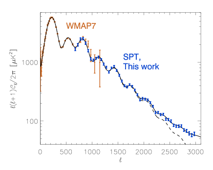
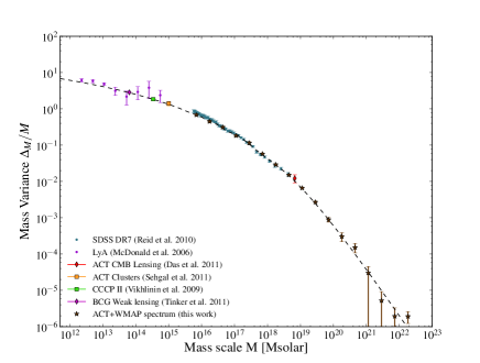
Figure 1: Left Panel: Recent CMBR angular power spectrum from the WMAP 7-year data and from the South Pole Telescope observations show as band-averaged powers along with the best fit $\Lambda$CDM model (CMB - dashed line) and (CMB + foreground solid line), taken from Ref. Ke11 . The detailed location, amplitude, and shape of the peaks (bumps) provide information on the contents of the Universe and the conditions at that early epoch plus secondary effects. Right panel: The mass variance of the reconstructed matter power spectrum from the Atacama Cosmology Telescope; large masses correspond to large scales and hence small values of $k$, taken from Ref. Hl11 . The BAO are barely visible in the detail of this arching spectrum driven by the damping, mostly at low mass, of the original perturbations during the oscillations.

References

- (1) G. Gamov, Phys. Rev. 70 (1946) 572; ibib 74 (1948) 505.
- (2) E. W. Kolb, and M. S. Turner, The Early Universe: Reprints, “Frontiers in Physics” # 70 (Addison-Wesley, 1988).
- (3) J. C. Mather et al, Astrophys. J. Lett. 354 (1990) L37.
- (4) G.F. Smoot et al, Astrophys. J. Lett. 396 (1992) L1.
- (5) N. Breton, J. L. Cervantes–Cota, and M. Salgado, Eds., An introduction to Standard Cosmology in The Early Universe and Observational Cosmology LNP 646 (Springer–Verlag, 2004).
- (6) L. Amendola and S. Tsujikawa, Dark energy: theory and observations (Cambridge University Press, 2010).
- (7) C.W. Misner, K.S. Thorne, and J.A. Wheeler, Gravitation (Freeman and Company, 1973).
- (8) A. Friedmann, Zeit. f. Phys. 10 (1922) 377; ibid 21 (1924) 326; H.P. Robertson, Astrophys. J. 82 (1935) 284; ibid 83 (1936) 187, 257; A.G. Walker, Proc. Lond. Math. Soc. (2) 42 (1937) 90.
- (9) E. P. Hubble, Proc. Nat. Acad. Sci. 15 (1929) 168.
- (10) N. Jarosik et al Astrophys. J. Suppl. 192 (2011) 14.
- (11) S. Weinberg, Rev. Mod. Phys. 61 (1989) 1.
- (12) S. Carrol, W. Press, and E. Turner, Ann. Rev. Astron. Astrophys. 30 (1992) 499.
- (13) S. Weinberg, Gravitation and Cosmology: principles and applications of the general theory of relativity (John Wiley & Sons, 1972); Cosmology (Oxford University Press, 2008).
- (14) C. M. Chambers and I. G. Moss, Phys. Rev. Lett. 73 617 (1994).
- (15) W. Rindler, Mon. Not. Roy. Astron. Soc. 116 (1956) 663.
- (16) E. J. Copeland, M. Sami, and S. Tsujikawa, Int. J. Mod. Phys. D15 (2006) 1753.
- (17) A. G. Riess et al., Astron. J. 116, (1998) 1009; Astron. J. 117 (1999) 707; S. Perlmutter et al., Astrophys. J. 517, (1999) 565.
- (18) R. Amanullah et al, Astrophys. J. 716 (2010) 712.
- (19) E.W. Kolb and M.S. Turner, The Early Universe “Frontiers in Physics” # 69 (Addison-Wesley, 1990).
- (20) R. H. Cyburt, B. D. Fields, K. A. Olive, E. Skillman, Astropart.Phys. 23 (2005) 313.
- (21) J.V. Narlikar, Introduction to Cosmology (Cambridge University press, Third Ed., 2002).
- (22) G. Steigman, Ann. Rev. Nucl Part. Sci. 29 (1979) 313.
- (23) W. de Sitter, Proc. Kon. Ned. Akad. Wet. 19 (1917) 1217; ibid 20 (1917) 229; Mon. Not. R. Astron. Soc. 76 (1916) 699; ibid 77 (1916) 155; ibid 78 (1917) 3.
- (24) G.W. Gibbons and S.W. Hawking, Phys. Rev. D 15 (1977) 2738.
- (25) A.D. Linde, Particle Physics and Inflationary Cosmology, (Harwood Ac., 1990).
- (26) A. Albrecht, P.J. Steinhardt, M.S. Turner, and F. Wilczek, Phys. Rev. Lett. 48 (1982) 1437; A.D. Dolgov and A.D. Linde, Phys. Lett. B 116 (1982) 329; L.F. Abbott, E. Farhi, and M.B. Wise, Phys. Lett. B 117 (1982) 29.
- (27) P.J. Steinhardt and M.S. Turner, Phys. Rev. D 29 (1984) 2162.
- (28) M.S. Turner, Phys. Rev. D 28 (1983) 1243.
- (29) A. R. Liddle and L. A. Urena-Lopez, Phys. Rev. Lett. 97 (2006) 161301.
- (30) J. H. Traschen and R.H. Brandenberger, Phys. Rev. D 42 (1990) 2491.
- (31) L. Kofman, A. Linde, and A.A. Starobinsky, Phys. Rev. Lett. 73 (1994) 3195; L. Kofman, A. Linde, and A.A. Starobinsky, Phys. Rev. Lett. 76 (1996) 1011.
- (32) G. N. Felder and L. Kofman, Phys. Rev. D 63 (2001) 103503.
- (33) A.D. Dolgov, Phys. Reports 222 (1992) 309; A. G. Cohen, D.B. Kaplan, and A.E. Nelson, Ann. Rev. Nucl. Part. Sci. 43 (1993) 27; J. L. Cervantes-Cota and H. Dehnen, Nucl. Phys. B 442 (1995) 391; M. Trodden, Rev. Mod. Phys. 71 (1999) 1463; F.L. Bezrukov and M. Shaposhnikov, Phys.Lett. B 659 (2008) 703.
- (34) S. Davidson, E. Nardi, and Y. Nir, Phys. Rept. 466 105 (2008).
- (35) B. A. Reid et al, Mon. Not. R. Astron. Soc. 404 (2010) 60.
- (36) J. Carlson, M. White, and N. Padmanabhan, Phys. Rev. D 80 (2009) 043531.
- (37) U. Seljak and M. Zaldarriaga. Phys. Rev. Lett. 78 (1997) 2054.
- (38) N. Turok, U.-L. Pen, and U. Seljak, Phys. Rev. D 58 (1998) 023506.
- (39) J. Kim and P. Naselsky, JCAP 7 (2009) 41.
- (40) V.F. Mukhanov, H.A. Feldman, and R.H. Brandenberger, Phys. Reports 215 (1992) 203.
- (41) C.-P. Ma and E. Bertschinger, Astrophys. J. 429 (1994) 22.
- (42) C.-P. Ma and E. Bertschinger, Astrophys. J. 455 (1995) 7.
- (43) D. H. Lyth and A. R. Liddle, The primordial density perturbation: cosmology, inflation and the origin of structure, (Cambridge University Press, 2009).
- (44) P. de Bernardis et al., Nature (London) 404 (2000) 955.
- (45) S. Hanany et al, Astrophys. J. 545 (2000) L5.
- (46) J. R. Bond, G. Efstathiou, and M. Tegmark, MNRAS 291 (1997) L33; M. Zaldarriaga, D. Spergel, and U. Seljak, ApJ 488 (1997) 1.
- (47) W. Hu and N. Sugiyama, Astrophys. J. 471 (1996) 542.
- (48) D. J. Eisenstein and W. Hu, Astrophys. J. 496 (1998) 605.
- (49) E. Komatsu et al Astrophys. J. Suppl. 180 (2009) 330.
- (50) H.-J. Seo and D. J. Eisenstein, Astrophys. J. 598 (2003) 720.
- (51) D. Schlegel et al, The BigBOSS Experiment, arXiv: 1106.1706.
- (52) D. J. Eisenstein et al, Astrophys. J. 633 (2005) 560.
- (53) A. Carnero et al, arXiv: 1104.5426.
- (54) R. Keisler et al, arXiv: 1105.3182.
- (55) R. Hlozek et al, arXiv: 1105.4887.