Abstract

The speed of computations is investigated by means of the orthogonality speed for a charged qubit interacting with a single cavity field prepared initially in a Fock state or Binomial state. We observe that the rate of the computational speed is related to the number of photons inside the cavity. Moreover, we show that the qubit-field coupling plays an opposite role, where the speed of computations is decreased as the coupling is increased. We suggest using the number of photons in the field as a control parameter to improve the speed of computations.

pacs74.70.-b, 03.65.Ta, 03.65.Yz, 03.67.-a, 42.50.-p

1 Introduction

In the last decade remarkable experiments were performed involving measurements and manipulations of states for a single or several nanoscopic Josephson junctions which were consistently interpreted in terms of two-level quantum systems [1-5]. Low-capacitance Josephson-junction devices have recently attracted a wide interest, both theoretically and experimentally, particularly in view of the possibility of identifying macroscopic quantum phenomena in their behavior. In this respect, one of the circuits that have gained great attention is the so-called Superconducting Cooper Pair Box (SCB), with an increasing number of experiments aimed at supporting a qubit interpretation of its evolution [6-9]. Several schemes have been proposed for implementing quantum computer hardware in solid state quantum electronics. These schemes use electric charge [10], magnetic flux [11] and superconducting phase [12] and electron spin [13].

The basic element of the quantum information is the quantum bit (qubit) which is considered as a two level system. In the quantum information and more precisely in the quantum computer, there is an important question which would be raised: what is the speed of sending information from a nod to another so as to reach the final output? Since the information is coded in a density operator, we therefore ask how fast the density operator will change its orthogonality [14]. This is to shed some light on the general behavior of the interaction process and its relationship with the speed of the computation [15-17] (maximum number of orthogonal states that the system can pass through per unit time), speed of orthogonality [18] (minimum time for a quantum state $\left|\Psi_{i}\right\rangle$ to evolve into orthogonal state $\left|\Psi_{f}\right\rangle$ where $\langle\Psi_{i}\left|\Psi_{f}\right\rangle=0$).

In the present paper, we consider the concrete situation of a two-level system (Cooper pair box) interacting with a quantum cavity field. We investigate the speed of computations when the initial state of the field is considered either in a Fock state or a binomial state. The following questions are considered: do useful properties of computational speed arise from considering different initial state settings? what role, if any, does mean photon number play any important role in the general behavior of the computational speed? and, in the framework of an initial binomial state, is it possible to obtain different orthogonality times which are useful for quantum computation? Answering these questions is the main aim of this paper.

The paper is organized as follows: in section II, we introduce a brief discussion on the qubit-field interaction and its dynamics. Section III is devoted to discuss the measures of the speed of the computations of typical bipartite states. Finally, discussion of the results and conclusion are given.

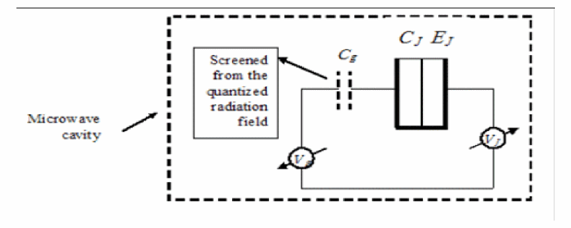
Figure 1: Schematic picture of the Cooper-pair box which is driven by an applied voltage, $Vg,$ through the gate capacitance, $Cg$. Black bars denote Cooper-pair box. The two Josephson junctions have capacitance, $C_{J},$ and Josephson energy, $E_{J}.$ The driving microwave field is generated using the electrical voltage acting on the charge qubit via the gate capacitance [11].

2 The model

We consider a superconducting box connected by a low-capacitance Josephson junction with capacitance $C_{J}$ and Josephson energy $E_{J}$, coupled capacitively to a gate voltage $V_{g}$ (gate capacitance $C_{g}$), placed inside a single-mode microwave cavity. We suppose that the gate capacitance $C_{g}$ is screened from the quantized radiation field (see figure (1)), and then the Hamiltonian of the system can be written as [19-21]

$$H=\frac{(Q-C_{g}V_{g}-C_{J}V)^{2}}{2(C_{g}+C_{J})}-E_{J}\cos\phi+\hbar\omega(a^{\dagger}a+\frac{1}{2}),$$ (1)

where $Q=2Ne$ is the Cooper pair charge on the island, where $N$ is the number of Cooper-pairs, $\phi$ is the phase difference across the junction, $\omega$ is the field frequency, and $a^{+}$, $a$ are the creation and annihilation operators of the microwave. $V$ is the effective voltage difference produced by the microwave across the junction. $V$ may be written down as [19-21]

$$V=i(\frac{\hbar\omega}{2C_{F}})^{\frac{1}{2}}(a-a^{\dagger}),$$ (2)

where $C_{F}$ is the capacitance parameter, which depends on the thickness of the junction, the relative dielectric constant of the thin insulating barrier, and the dimension of the cavity. Here, we consider the case where the charging energy with scale $E_{c}=\frac{e^{2}}{2(C_{g}+C_{J})}$ dominate over the Josephson coupling energy $E_{J}$ , and concentrate on the value $V_{g}=\frac{e}{C_{g}}$ and weak quantized radiation field, so that only the two low-energy charge states $N=0$ and $N=1$ are relevant. In this case the Hamiltonian in a basis of the charge state $\left|\downarrow\right\rangle$ and $\left|\uparrow\right\rangle$ reduces to a two-state form in a spin- $1/2$ language [10,23-24]

$$H=E_{c}(1+\frac{C_{J}^{2}V^{2}}{e^{2}})-2E_{c}\frac{C_{J}V}{e}J_{z}-\frac{1}{2}E_{J}J_{x}+\hbar\omega(a^{\dagger}a+\frac{1}{2}).$$ (3)

We denote by $J_{z}$ and $J_{x}$ the Pauli matrices in the pseudo-spin basis {$\left|\downarrow\right\rangle$, $\left|\uparrow\right\rangle$},

$$J_{x}=\left|\uparrow\right\rangle\left\langle\downarrow\right|+\left|\downarrow\right\rangle\left\langle\uparrow\right|\mbox{ and }J_{z}=\left|\uparrow\right\rangle\left\langle\uparrow\right|-\left|\downarrow\right\rangle\left\langle\downarrow\right|\mbox{},$$ (4)

where the charge states are not the eigenstates of the Hamiltonian (3), even in the absence of the quantized radiation field, i.e.$V=0$, we describe $H$ in the two charge states subspace through new states and denote the corresponding states as $\left|+\right\rangle$ and $\left|-\right\rangle$ [24] as

$$\left|+\right\rangle=\frac{1}{\sqrt{2}}(\left|\uparrow\right\rangle-\left|\downarrow\right\rangle)\mbox{, }\left|-\right\rangle=\frac{1}{\sqrt{2}}(\left|\uparrow\right\rangle+\left|\downarrow\right\rangle).$$ (5)

In the weak quantized radiation field, one may neglect the term containing $V^{2}$ in equation (3) and from Eqs. (1-5), the Hamiltonian in the new basis $\left|+\right\rangle$ and $\left|-\right\rangle$ is given by

$$H=E_{c}-2iE_{c}\frac{C_{J}}{e}(\frac{\hbar\omega}{2C_{F}})^{\frac{1}{2}}(a-a^{\dagger})\sigma_{x}+\frac{1}{2}E_{J}\sigma_{z}+\hbar\omega(a^{\dagger}a+\frac{1}{2}).$$ (6)

We denote by $\sigma_{z}$ the Pauli matrix, $\sigma_{+}$ and $\sigma_{-}$ the raising and lowering operators ($\left[\sigma_{+},\sigma_{-}\right]=\sigma_{z}$). In the rotating wave approximation,the Hamiltonian takes the following form

$$H=E_{c}+\frac{1}{2}E_{J}\sigma_{z}+i\hbar g(a\mbox{ }\sigma_{+}-a^{\dagger}\sigma_{-})+\hbar\omega(a^{\dagger}a+\frac{1}{2})\mbox{,},$$ (7)

where

$$g = (\frac{\omega}{C_{F}\hbar})^{\frac{1}{2}}\frac{E_{c}}{2}$$ (8)

$$= (\frac{\omega}{2C_{F}\hbar})^{\frac{1}{2}}\frac{eC_{J}}{(C_{g}+C_{J})}\mbox{.}.$$ (9)

It is noted that the Hamiltonian (7) is just like the simplest form of atom- field interaction, which is known as the Jaynes-Cummings model (JCM) [25]. In this paper we consider the case where $E_{J}\sim\hbar\omega<<E_{c}$ then, in the interaction picture, the Hamiltonian (7) takes the form ($\hbar=1$),

$$H_{I}^{I}=\frac{1}{2}\Delta\sigma_{z}+ig(a\mbox{ }\sigma_{+}-a^{\dagger}\sigma_{-}),$$ (10)

where $\Delta=E_{J}-\omega$ is the detuning between the Josephson energy and cavity field frequency. We shall be working from now on in the basis $\left\{\left|+\right\rangle,\left|-\right\rangle\right\}$, then in the interaction picture, the Hamiltonian (9) is written as [26]

$$H_{I}^{I}=\left(\begin{array}[]{cc}\frac{\Delta}{2}&-iga\\ iga^{\dagger}&-\frac{\Delta}{2}\end{array}\right),$$ (11)

and the corresponding evolution operator $U_{t}=\exp(-iH_{I}^{I}t)$ can be written in the form

$$U_{t}=\left(\begin{array}[]{cc}U_{11}(t)&U_{12}(t)\\ U_{21}(t)&U_{22}(t)\end{array}\right),$$ (12)

where

$$U_{11}(t) = \cos\Omega_{n+1}t-i\frac{\Delta}{2}\frac{\sin\Omega_{n+1}t}{\Omega_{n+1}},$$

$$U_{12}(t) = iga\frac{\sin\Omega_{n}t}{\Omega_{n}},$$

$$U_{22}(t) = \cos\Omega_{n}t+i\frac{\Delta}{2}\frac{\sin\Omega_{n}t}{\Omega_{n}},$$ (13)

with, $\Omega_{n}=(\frac{\Delta^{2}}{4}+g^{2}n)^{2},n=a^{\dagger}a$ and $U_{21}=U_{12}^{\dagger}$. The density operator at any time, $t>0,$ is given by

$$\rho_{I}(t)=U_{t}\rho(0)U_{t}^{\dagger},$$ (14)

where$\rho(0)=\rho_{b}(0)\otimes\rho_{f}(0)$. Having obtained the density operator at any time, $t\geq 0$ ,one can investigate the speed of computation as described in the following sections.

3 The speed of computation

We shall assume that the box is initially in its pure state, that is

$$\rho_{b}(0)=\frac{1}{2}\left(\begin{array}[]{cc}1&1\\ 1&1\end{array}\right),$$ (15)

with eigenvectors

$$\nu_{\pm}=\frac{1}{\sqrt{2}}\left(\begin{array}[]{c}1\\ \pm 1\end{array}\right).$$ (16)

Using this initial state, the density operator at any time, $t>0,$ is given by

$$\rho_{I}(t)=\left(\begin{array}[]{cc}\rho_{11}(t)&\rho_{12}(t)\\ \rho_{21}(t)&\rho_{22}(t)\end{array}\right),$$ (17)

where,

$$\rho_{11}(t) = \frac{1}{2}(U_{11}\rho_{f}(0)U_{11}^{\dagger}+U_{12}\rho_{f}(0)U_{11}^{\dagger}+U_{11}\rho_{f}(0)U_{12}^{\dagger}+U_{12}\rho_{f}(0)U_{12}^{\dagger}),$$

$$\rho_{12}(t) = \frac{1}{2}(U_{11}\rho_{f}(0)U_{21}^{\dagger}+U_{12}\rho_{f}(0)U_{21}^{\dagger}+U_{11}\rho_{f}(0)U_{22}^{\dagger}+U_{12}\rho_{f}(0)U_{22}^{\dagger}),$$

$$\rho_{22}(t) = \frac{1}{2}(U_{21}\rho_{f}(0)U_{21}^{\dagger}+U_{22}\rho_{f}(0)U_{21}^{\dagger}+U_{21}\rho_{f}(0)U_{22}^{\dagger}+U_{22}\rho_{f}(0)U_{22}^{\dagger}),$$ (18)

and $\rho_{21}(t)=\rho^{*}_{12}(t)$.

3.1 Initial Fock State

Now we assume that the field is initially in a Fock state, that is $\rho_{f}(0)=\left|n\right\rangle\left\langle n\right|$, then one can calculate $\rho_{ij}^{b}(t)$ by calculating $Tr_{f}(U\rho_{f}(0)U^{\dagger})_{ij}$, The elements of the density operator are given by,

$$\rho^{b}_{11}(t) = \frac{1}{2}\Bigl{(}\cos^{2}\Omega_{n+1}t+(\frac{\Delta}{2})^{2}\frac{\sin^{2}\Omega_{n+1}t}{\Omega_{n+1}^{2}}+g^{2}n\frac{\sin^{2}\Omega_{n}t}{\Omega_{n}^{2}}\Bigr{)},$$

$$\rho^{b}_{22}(t) = \frac{1}{2}\Bigl{(}\cos^{2}\Omega_{n}t+(\frac{\Delta}{2})^{2}\frac{\sin^{2}\Omega_{n}t}{\Omega_{n}^{2}}+g^{2}(n+1)\frac{\sin^{2}\Omega_{n+1}t}{\Omega_{n+1}^{2}}\Bigr{)},$$

$$\rho^{b}_{12}(t) = \frac{1}{2}\Bigl{(}\cos\Omega_{n+1}t-i\frac{\Delta}{2}\frac{\sin\Omega_{n+1}t}{\Omega_{n+1}})(\cos\Omega_{n}t-i\frac{\Delta}{2}\frac{\sin\Omega_{n}t}{\Omega_{n}}\Bigr{)}.$$ (19)

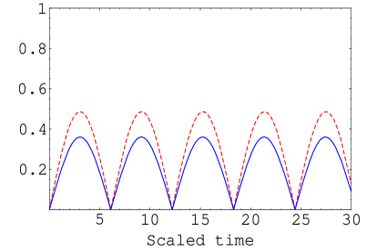
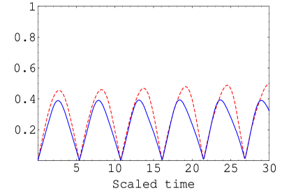
Figure 2: The speed of orthogonality for $\Delta=n=1$ (a) $g=0.1$ and (b) $g=0.25$, (c) $g=0.35$ and (d)$g=0.5$.

Direct calculations can be used to obtain the eigenvectors $u_{1,2}(t)$ for the final state $\rho^{b}(t),$ we can explicitly write $u_{1,2}(t)$ as the follows

$$u_{1,2}(t)=\pm\sqrt{\frac{\left|\rho^{b}_{12}(t)\right|^{2}}{\left|\rho^{b}_{12}(t)\right|^{2}+\left|\lambda_{1,2}(t)-\rho^{b}_{11}(t)\right|^{2}}}\left(\begin{array}[]{c}1\\ \frac{(\lambda_{1,2}(t)-\rho^{b}_{11}(t))}{\rho^{b}_{12}(t)}\end{array}\right),$$ (20)

where

$$\lambda_{1,2}(t)=\frac{1}{2}\left(1\pm\sqrt{(\rho^{b}_{11}(t)-\rho^{b}_{22}(t))^{2}+4\left|\rho^{b}_{12}(t)\right|^{2}}\right).$$ (21)

In order to facilitate our discussion, let us define the scalar product of the vectors $u_{i}(t)$ and $\nu_{j}(0)$ such as

$$Sp_{ij}=\langle\nu_{i}(0)\left|u_{j}(t)\right\rangle,$$ (22)

where $\nu_{i}$ and $u_{j}$ represent the eigenvectors of the initial and final state of the Cooper-pair box. The expression $Sp_{ij}$ represents the dot product of the four possibilities i.e $Sp_{11}=\langle\nu_{1}(0)\left|u_{1}(t)\right\rangle$, $Sp_{12}=\langle\nu_{1}(0)\left|u_{2}(t)\right\rangle$. If the dot product for any two eigenvectors vanishes this means that the two vectors are orthogonal and the information which is coded in one eigenvector is transformed to the other eigenvector. The number of vanishing eigenvectors indicates speed of orthogonality and consequently the speed of computations.

It should be noted that in our calculations we have taken into account all the possible products of $u_{i}$ and $\nu_{j}$, but we produce the best figures in all the possible products of $u_{i}$ and $\nu_{j}$. In what follows we present the dynamics of the amplitude values of $Sp_{ij}$ which represents the speed of orthogonality against the scaled time for different values of the field and the Cooper pair parameters.

In Fig. 2, we investigate the effect of the coupling constant $g$ on the speed of orthogonality $Sp_{ij}$, where, we set $\Delta=n=1$. It is clear that for small values of the coupling constant, $g$, the speed of orthogonality is very large. As the coupling constant is increased the speed of orthogonality is decreased. However for $g>0.5$, the speed is almost zero.

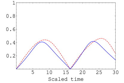
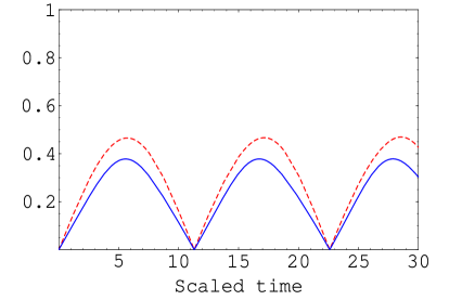
Figure 3: The effect of the detuning parameter on the speed of orthogonality. The parameters are $n=1$, $g=0.1$ and different values of detuning, where, (a)$\Delta=0.3$ (b) $\Delta=0.5$ and (c) $\Delta=1$, (d) $\Delta=2$.

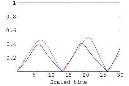
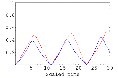
Figure 4: The effect of the number of photons on the speed of orthogonality, where $g=0.1$, $\Delta=0.3$(a)$n=3$ (b) $n=5$ and (c) $n=10$, (d) $n=20$.

Fig. 3 shows the dynamics of orthogonality speed for different values of the detuning parameter, where the other parameters are assumed to be constant. In Fig. 3a we set a small value of the detuning parameter $\Delta=0.3$, while the number of photons $n=1$ and the coupling constant $g=0.1$. It is clear that the orthogonality appears only one time. However as one increases the detuning, $\Delta=0.5,$ as shown in Fig. 3b, the amplitude of $Sp_{ij}$ vanishes at a specific time in this range of the scaled time. This means that the speed of orthogonality is increased. Further increase of the detuning parameter, the number of zeros of the amplitudes of $Sp_{ij}$ is increased and consequently the speed of orthogonality is increased as shown in Fig. 3c and Fig.3d, where we set $\Delta=1$ and $\Delta=2,$ respectively.

Now, let us investigate the effect of the field parameter which is represented by the number of photons $n$ on the speed of orthogonality. In Fig. 4, we consider different values of the photon number $n$, while we consider the values of the other parameters such that the speed of orthogonality is very small. Fig. 4a displays the dynamical behavior of the amplitude $Sp_{ij}$ for $n=3$. One sees that, this amplitude vanishes once, which means that the orthogonality appears another time (see Fig. (3a), where $n=1$). This means that the speed of orthogonality is increased as one increases the number of photon $n$. This remark appears clearly in Fig. 4b, Fig. 4c and Fig. 4d, where we set $n=5,10$ and $20,$ respectively.

From Figs. 2 and 3, it is clear that as one increases the coupling constant, $g$, i.e., the ratio $C_{j}/(C_{g}+C_{j})$ is increased, the possibility of increasing the speed of orthogonality is lower. One can overcome this problem by increasing the detuning parameter. However, it may be difficult to control the parameters $g$ and $\Delta$, but it will be more easy to control the number of photons $n$. In this case, by increasing the number of photons one can increases the speed of orthogonality and consequently the speed of computation. Therefore, one can look at these parameters as control parameters to improve the speed of computations.

3.2 Initial Binomial State

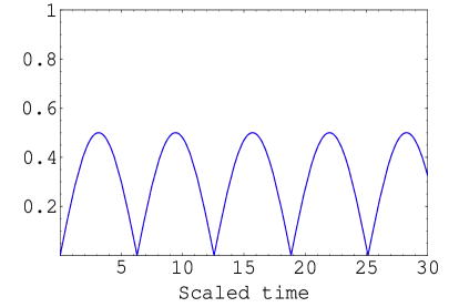
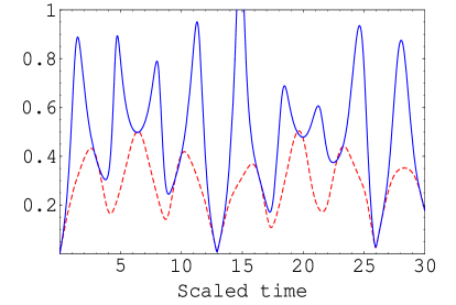
Figure 5: The speed of orthogonality for a Cooper pair interact with a field in prepared initially in a binomial state, where $\Delta=1$ and $\eta=0.1$ (a) $g=0.001$ and (b) $g=0.8$.

In this case, we assume that the field is initially prepared in a binomial state,

$$\rho_{f}(0)=\left|\mu,\eta\right\rangle\left\langle\eta,\mu\right|$$ (23)

where

$$\left|\mu,\eta\right\rangle=\sum_{m=0}^{\mu}\sqrt{\kappa}\eta^{m}(1-\left|\eta\right|^{2})^{\frac{\mu-m}{2}}\left|m\right\rangle,\quad\kappa=\frac{\mu!}{m!(\mu-m)!},\mu\mbox{ an integer, }\left|\eta\right|\leq 1,$$ (24)

the coherent state is obtained when $(\mu\rightarrow\infty,$and $\left|\eta\right|\rightarrow 0$ such that $\mu\eta^{2}\rightarrow\tilde{n}=\left|\alpha\right|^{2}).$The time evaluation of the density operator of the charged qubit and the field, $\rho(t),$ is obtained by using (23) and the unitary operator (2). Tracing out the field state, one obtains the time evolution of the qubit state, namely, $\rho_{ij}^{b}(t)=Tr_{f}(U\rho_{f}(0)U^{\dagger})_{ij}$. The elements of this density operator are given by,

$$\rho_{11}(t) = \sum_{n=0}^{\mu}\Upsilon\eta^{2n}(1-\left|\eta\right|^{2})^{\mu-n}[\cos^{2}\Omega_{n+1}t+g^{2}n\frac{\sin^{2}\Omega_{n}t}{\Omega_{n}^{2}}$$

$$+(\frac{\Delta}{2})^{2}\frac{\sin^{2}\Omega_{n+1}t}{\Omega_{n+1}^{2}}-2g\frac{(\mu-n)}{\sqrt{n+1}}\eta(1-\left|\eta\right|^{2})^{-\frac{1}{2}}\cos\Omega_{n+1}t\frac{\sin\Omega_{n}t}{\Omega_{n}}],$$

$$\rho_{22}(t) = \sum_{n=0}^{\mu}\Upsilon\eta^{2n}(1-\left|\eta\right|^{2})^{\mu-n}[\cos^{2}\Omega_{n}t+g^{2}(n+1)\frac{\sin^{2}\Omega_{n+1}t}{\Omega_{n+1}^{2}}$$

$$+(\frac{\Delta}{2})^{2}\frac{\sin^{2}\Omega_{n}t}{\Omega_{n}^{2}}-2g\frac{(\mu-n)}{\sqrt{n+1}}\eta(1-\left|\eta\right|^{2})^{-\frac{1}{2}}\cos\Omega_{n+1}t\frac{\sin\Omega_{n+1}t}{\Omega_{n+1}}],$$

$$\rho_{12}(t) = \sum_{n=0}^{\mu}\Upsilon\eta^{2n}(1-\left|\eta\right|^{2})^{\mu-n}[(\cos\Omega_{n+1}t-i\frac{\Delta}{2}\frac{\sin\Omega_{n+1}t}{\Omega_{n+1}})(\cos\Omega_{n}t$$ (25)

$$-i\frac{\Delta}{2}\frac{\sin\Omega_{n}t}{\Omega_{n}})-g^{2}\frac{(\mu-n)}{\sqrt{n+1}}\frac{(\mu-n+1)}{\sqrt{n+2}}(1-\left|\eta\right|^{2})^{-1}\frac{\sin\Omega_{n+1}t}{\Omega_{n+1}}\frac{\sin\Omega_{n+2}t}{\Omega_{n+2}}$$

$$+g\frac{(\mu-n)}{\sqrt{n+1}}\eta(1-\left|\eta\right|^{2})^{-\frac{1}{2}}\frac{\sin\Omega_{n+1}t}{\Omega_{n+1}}[(\cos\Omega_{n}t-\cos\Omega_{n+2}t)$$

$$+i\frac{\Delta}{2}(\frac{\sin\Omega_{n}t}{\Omega_{n}}-\frac{\sin\Omega_{n+2}t}{\Omega_{n+2}})]],$$

where $\Upsilon=\frac{\mu!}{(\mu-n)!n!}$. Using the obtained density operator of the system, we calculate the speed of orthogonality and consequently the computational speed.

The effect of the coupling constant on the speed of orthogonality for a Cooper pair interacts with a cavity mode initially prepared in the binomial state is described in Fig.5. It is clear that, as one increases the coupling constant the speed of orthogonality decreases, where the numbers of vanishing amplitudes $Sp_{ij}$ increases for larger values of $g$. However for $g>1$, the amplitudes $Sp_{ij}$ oscillate very fast but the number of orthogonality decreases.

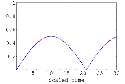
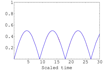
Figure 6: The same as Fig.(4), where $g=0.01,\eta=0.1$ and (a) $\Delta=0.3$ and (b) $\Delta=0.7$, (c) $\Delta=1$ and (d)$\Delta=2$.

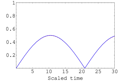
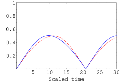
Figure 7: The same as Fig.(4), where $g=0.01$, $\Delta=0.3$ and (a) $\eta=0.001$ and (b) $\eta=0.8$.

Fig.6 describe the dynamics of the amplitudes $Sp_{ij}$ for different values of the detuning parameter while the other parameters are assumed to be fixed. It is clear that, for small value of the detuning, $\Delta=0.3$ the number of vanishing $Sp_{ij}$ is small and consequently the speed of orthogonality. However as one increases the detuning the speed of orthogonality increases and consequently the speed of computations. On the other hand, if we compare Fig. 6a, where $\Delta=0.3$ and Fig. 6b, where $\Delta=0.5$, we can see that the amplitudes $Sp_{ij}$ vanishes two times for the latter case. Moreover, the orthogonality time, the time in which the amplitudes vanish, is shorter than that depicted in Fig. 6a. However, for larger values of the detuning parameter the orthogonality time decreases more and consequently the computational time, the time which is taken to transfer the information from one node to another, decreases. Therefore, it will be enough to investigate the effect of the parameter $\eta$ on the orthogonality speed. Fig.7, displays the dynamics of $Sp_{ij}$ for different values of the parameter $\eta$. In Fig. 7a, we set a small value of $\eta,$ (say $\eta=0.001)$, while the other parameters are fixed. However the speed of orthogonality doesn’t affected as one increases $\eta$ (See Fig.(7b), where we set $\eta=0.8$).

4 Conclusion

The dynamics of a charged qubit interacts with a cavity mode prepared initially in either Fock state or Binomial states is investigated. The computational speed is studied by means of the orthogonality speed. The effect of the field and the charged qubit parameters is investigated. We show that, the detuning parameter and the number of photons inside the cavity play essential roles on controlling the speed of orthogonality and consequently the computational speed. However, larger values of the detuning and the number of photons, lead to increase the number of orthogonality and decrease the orthogonality time and consequently decrease the computational time, i.e., the speed of computations is increased. On the other hand, the effect of the the coupling between the charged qubit and the cavity mode is different. It is shown that, as one increases the coupling parameter, the number of orthogonality is increased and the orthogonality time is increased, i.e., the speed of computation is decreased.

For binomial case, the parameter $\eta$, has almost no effect on the speed of orthogonality, while the coupling constant between the field and the Cooper pair has a noticeable effect. For a large value of $g$, the number of orthogonality is decreased and consequently the computational speed is decreased.

Acknowledgement: we are grateful for the helpful comments given by the referees.

References

• [1] G. Wendin and V. S. Shumeiko, in Handbook of theoretical and Computational Technology, Edited by M. Rieth and W. Schommers, American Scientific Publishers (2005).
• [2] Y. Nakamura, Yu. A. Pashkin and J.S. Tsai, Nature 398 (1999) 786.
• [3] K. Bladh, T. Duty, D. Gunnarsson and P. Delsing, New Journal of Physics 7 (2005) 180.
• [4] K. W. Lehnet et al., Phys. Rev. Lett. 90 (2003) 027002.
• [5] Ansmann M et al., Nature 461 (2009) 504.
• [6] Y. Nakamura, Yu.A. Pashkin and J.S. Tsai, Phys. Rev. Lett. 87 (2001) 246601.
• [7] T. Yamamoto, Y. A. Pashkin, O. Astafiev and Y. Nakamura and J.S. Tsai, Nature 425 (2003) 941
• [8] A. J. Berkeley, H. Xu, R. C. Ramos, M. A. Gubrud, F. W. Strauch, P. R. Johnson, J. R Anderson, A. J. Dragt, C. J. Lobb and F. C. Wellstood, Science 300 (2003) 1548.
• [9] M. Steffen, M. Ansmann, R. C. Bialczak, N. Katz, E. Lucero, R. McDermott, M. Neeley, E. M. Weig, A. N. Cleland and J. M. Martinis, Science 313 (2006) 1423; N. Metwally and A. A. Al-Amin Physica E, 41 718-722 (2009).
• [10] D. V. Averin, Solid State Communications, 105 659 (1998); Y. Makhlin, G.Schon, and A. Shnirman, Nature 398 (1999) 305.
• [11] J. Mooij, T. Orlando, L. Levitov, L. Tian, C. H. van der Wal, and S. Lloyd, Science 285 (1999) 1036.
• [12] A. Blais, A. Zagoskin Phy. Rev. A, 61 (2000) 042308.
• [13] D. Loss, D. DiVincenzo, Phys. Rev. A 57 (1998) 120.
• [14] N. Metwally, M. Abdel-Aty, M. S. Abdalla, I.J. Mod. Phys. B, 22, No. 24 (2008) 4143-4151.
• [15] N. Margolus and L. B. Levitin, Physica D, 120 (1998) 188.
• [16] J. Batle, M. Casas, A. Plastino and A. R. Plastino, Phys. Rev. A, 72 (2005) 032337.
• [17] A. Borrs, M. Casas, A. R. Plastino and A. Plastino, Phys. Rev. A, 74 (2006) 022326.
• [18] M.-H. Yung, Phys. Rev. A, 74 (2006) 030303(R).
• [19] R. Migliore, A. Messina and A. Napoli, Eur. Phys. J. B,13 (2000) 585; 22 (2001) 111.
• [20] Y.-S. Yao, J. Zou and B. Shao, Chin. Phys., 11 (2002) 1200.
• [21] M. Zhang, J. Zou and B. Shao, Int. J. Mod. Phys., B 16 (2002) 4767.
• [22] M. Zhang , J. Zou and B. Shao, Int. J. Mod. Phys. B, 17, (2003) 2699.
• [23] A. Shnirman, G. Schon and Z. Hermon, Phys. Rev. Lett., 79 (1997) 2371.
• [24] W. Krech and Th. Wagner, Phys. Lett. A, 275 (2000) 159.
• [25] E. T. Jaynes and F. W. Cummings, Proc. IEEE, 51 (1963) 89; F. W. Cummings, Phys. Rev., 140 (1965) A1051; P. Meystre, A. Quattropani and H. P. Bates, Phys. Lett., 49A (1974) 85.
• [26] V. Buzek, H. Moya-Cessa, P. L. Knight and S. J. D. Phoenix, Phys. Rev. A, 45 (1992) 8190.