The cryptohermitian smeared-coordinate representation of wave functions

Miloslav Znojil

Nuclear Physics Institute ASCR,

250 68 Řež, Czech Republic

e-mail: znojil@ujf.cas.cz

Abstract

In discrete-coordinate quantum models the kinematical observable of position need not necessarily be chosen local (i.e., diagonal). Its smearing is selected in the nearest-neighbor form of a real asymmetric (i.e., cryptohermitian) tridiagonal matrix $\hat{Q}$. Via Gauss-Hermite illustrative example we show how such an option restricts the class of admissible dynamical observables (sampled here just by the Hamiltonian).

1 Introduction

Virtually any textbook on quantum mechanics pays attention to the point particle moving along straight line. Tacitly [1], it is assumed that the argument $x$ of its wave function $\psi(x)\in L^{2}(\mathbb{R})$ coincides with an eigenvalue of an operator of the (by assumption, observable) spatial position. The wave functions $\psi(x)$ carry the standard probability-density interpretation and describe the system in the so called $x-$representation.

For Hamiltonians $H=p^{2}+V(x)$ in which the external potential is local, such an approach is natural. Due to the second-order differential-operator form of $H$, one easily determines the energies. The calculations may be further facilitated by the transition to approximations. Typically [2], the equidistant $N-$point Runge-Kutta discretization

$$x\in\mathbb{R}\ \ \longrightarrow\ \ x_{j}=x_{j}^{(RK)}=x_{0}^{(RK)}+h\cdot j\,,\ \ \ \ \ h>0\,,\ \ \ {j=0,1,\ldots,N-1}$$

converts operator $H$ into a real and symmetric tridiagonal $N$ by $N$ matrix.

For non-local external potentials the concept of the coordinate loses its guiding role of a link between the quantum and classical pictures while the kinetic energy operator $p^{2}$ may still be simplified via Fourier transformation ${\cal F}:\,\psi(x)\,\to\,\tilde{\psi}(p)$. Thus, unless one has to deal with some other observables defined as functions of $x$, the computing costs of the mapping ${\cal F}$ remain acceptable.

The feasibility of the calculations worsens for the more complicated Hamiltonians $H\neq p^{2}+V$ so that the role of the quality of the approximations increases. In particular, the Runge-Kutta grid points $x_{j}=x_{j}^{(RK)}$ may prove far from optimal in practice [3]. Many non-Runge-Kutta discretizations are being proposed and used in physics and quantum chemistry, therefore [4].

Table 1: The sample of the closed-form grid points $x_{j}^{(HP)}$ at $N\leq 5$

$N$	$q_{0}$	$q_{1}$	$q_{2}$	$q_{3}$	$q_{4}$	…
1	0
2	$-{}{\sqrt{2}}{}$	${}{\sqrt{2}}{}$
3	$-{}{\sqrt{6}}{}$	0	${}{\sqrt{6}}{}$
4	$-{}{\sqrt{6+2\,\sqrt{6}}}{}$	$-{}{\sqrt{6-2\,\sqrt{6}}}{}$	${}{\sqrt{6-2\,\sqrt{6}}}{}$	${}{\sqrt{6+2\,\sqrt{6}}}{}$
5	$-{}{\sqrt{10+2\,\sqrt{10}}}{}$	$-{}{\sqrt{10-2\,\sqrt{10}}}{}$	0	${}{\sqrt{10-2\,\sqrt{10}}}{}$	${}{\sqrt{10+2\,\sqrt{10}}}{}$
⋮	…

In our forthcoming methodical considerations one of the most typical samples of the non-Runge-Kutta one-dimensional grid points will be selected in the form of the $N-$plet of the zeros of the $N-$th Hermite polynomial [5],

$$x\in\mathbb{R}\ \ \longrightarrow\ \ x_{j}=x_{j}^{(HP)}\,,\ \ \ \ \ \ {j=0.1,\ldots,N-1}\,.$$ (1)

In a way explained in Appendix A we felt puzzled by the conflict between the amendment of the numerical efficiency gained by the transition from $x_{j}^{(RK)}$ to $x_{j}^{(HP)}$ (cf. Refs. [5, 6] for details) and the loss of the closed formulae for $x_{j}^{(HP)}$ (with a few low$-N$ exceptions sampled in Table 1). A softening of the latter disadvantage (i.e., of the purely numerical character of the amended values $x_{j}^{(HP)}$ at higher $N$) will be proposed here, therefore.

In section 2, first of all, the numerical values of $x_{j}^{(HP)}$ will be reinterpreted as the implicitly defined eigenvalues of a suitable tridiagonal matrix $\hat{Q}^{(N)}$ with elementary matrix elements. It will be argued there that one of versions of such a next-to-diagonal form of $\hat{Q}^{(N)}$ is in fact often used during the evaluation of values $x_{j}^{(HP)}$ in numerical practice.

In section 3 (complemented also by Appendix B) our specific choice of manifestly non-Hermitian $N$ by $N$ matrices $\hat{Q}^{(N)}$ will be advocated. Their extreme simplicity will be identified there with the main criterion of applicability of the increasingly popular use of representations of quantum observables (sampled here by the position and energy) in the so called cryptohermitian picture.

In section 4, the main formal aspects and consequences of the use of the grid $x_{j}^{(HP)}$ in such an implicit representation will be explained, in detail, via the first nontrivial $N=4$ model. The abstract picture of kinematics (represented by the matrix $\hat{Q}^{(N)}$) and dynamics (represented by the related admissible families of Hamiltonians $H^{(N)}$ and/or of the so called metric operators $\Theta^{(N)}$) will be given there the concrete forms in which the construction of matrices $\Theta^{(N)}$ in the simplest (viz., tridiagonal and pentadiagonal) sparse-matrix forms will be paid particular attention.

In the final section 5 the resulting change of perspective transferring emphasis from the simplicity of quantum kinematics to a potentially better balance between the simplicity of kinematics and dynamics will be summarized.

2 Formalism: Kinematics

2.1 An implicit definition of grid points $x_{j}^{(HP)}$

Let us consider the classical orthogonal Hermite polynomials

$$H_{0}(x)=1\,,\ \ \ H_{1}(x)=2\,x\,,\ \ \ H_{2}(x)=4\,{x}^{2}-2\,,\ \ \ H_{3}(x)=8\,{x}^{3}-12\,x\,,\ldots\,$$ (2)

and make our present grid points $x_{j}^{(HP)}$ unique by defining them as the roots of equation

$$H_{N}\left(\frac{1}{2}\,x_{j}^{(HP)}\right)=0\,,\ \ \ \ j=0,1,\ldots\,,N-1\,.$$ (3)

Naturally, such a definition of the grid points is purely numerical, at the larger lattice-sizes $N$ at least. At the finite $N$, there is in fact no practical necessity of insisting on the multiplicative-operator nature (i.e., on the diagonal matrix form and representation) of the position-operator $\hat{Q}=\hat{Q}^{(N)}$. Thus, once we re-read our implicit lattice-definition (3) as a vanishing-condition for the determinant of recurrences for Hermite polynomials we may immediately replace the traditional and, in essence, purely numerical diagonal representation of the operator $\hat{Q}^{(N)}$ by its following, well known tridiagonal-matrix alternative

$$\hat{Q}^{(N)}=\left[\begin{array}[]{cccccc}0&1&0&0&\ldots&0\\ \vskip 6.0pt plus 2.0pt minus 2.0pt\cr 2&0&1&0&\ddots&\vdots\\ \vskip 6.0pt plus 2.0pt minus 2.0pt\cr 0&4&0&\ddots&\ddots&0\\ \vskip 6.0pt plus 2.0pt minus 2.0pt\cr 0&0&6&\ddots&1&0\\ \vskip 6.0pt plus 2.0pt minus 2.0pt\cr\vdots&\ddots&\ddots&\ddots&0&1\\ \vskip 6.0pt plus 2.0pt minus 2.0pt\cr 0&\ldots&0&0&{2N-2}&0\end{array}\right]\,.$$ (4)

The proof of the coincidence of the eigenvalues of this matrix with the roots of Eq. (3) is easy - it suffices to recall the recurrences for Hermite polynomials [7]. Subsequently, we may even specify the related eigenvectors of matrix (4), i.e., the smeared position eigenstates in closed form,

$$|\psi_{n}\rangle=\left(\begin{array}[]{c}H_{0}(x_{n}/2)\\ H_{1}(x_{n}/2)\\ \vdots\\ H_{N-1}(x_{n}/2)\end{array}\right)\,,\ \ \ \ \ n=0,1,\ldots\,,N-1\,.$$ (5)

In such an overall setting one has to circumvent several conceptual as well as purely technical obstacles. Some of them will be discussed in what follows.

2.2 A trivial Hermitization of $\hat{Q}^{(N)}$

As long as we have $\hat{Q}^{(N)}\neq\left[\hat{Q}^{(N)}\right]^{\dagger}$ we must abandon the “friendly” real vector space ${\cal H}^{(F)}=\mathbb{R}^{N}$ as unphysical. At the same time we may introduce a diagonal $N$ by $N$ matrix $\Omega^{(N)}_{0}$ with positive matrix elements along its diagonal, $\left[\Omega^{(N)}_{0}\right]_{mn}=\omega_{n}\delta_{mn}$. This enables us to define matrix

$$\mathfrak{q}^{(N)}_{0}=\Omega^{(N)}_{0}\hat{Q}\left[\Omega^{(N)}_{0}\right]^{-1}\,$$ (6)

possessing the same eigenvalues as $\hat{Q}$. As long as the original position operator $\hat{Q}$ itself is a tridiagonal matrix, we are allowed to require that our grid-points-preserving similarity transformation (6) has the Hermitization property,

$$\mathfrak{q}^{(N)}_{0}=\left[\mathfrak{q}^{(N)}_{0}\right]^{\dagger}\,.$$

We may put $\omega_{n}=c/\sqrt{(2n)!!}$ at any $c\neq 0$ and $n=0,1,\ldots,N-1$ yielding the closed and well known formula

$$\mathfrak{q}^{(N)}_{0}=\left[\begin{array}[]{cccccc}0&\sqrt{2}&0&0&\ldots&0\\ \vskip 6.0pt plus 2.0pt minus 2.0pt\cr\sqrt{2}&0&\sqrt{4}&0&\ddots&\vdots\\ \vskip 6.0pt plus 2.0pt minus 2.0pt\cr 0&\sqrt{4}&0&\ddots&\ddots&0\\ \vskip 6.0pt plus 2.0pt minus 2.0pt\cr 0&0&\sqrt{6}&\ddots&\sqrt{2N-4}&0\\ \vskip 6.0pt plus 2.0pt minus 2.0pt\cr\vdots&\ddots&\ddots&\ddots&0&\sqrt{2N-2}\\ \vskip 6.0pt plus 2.0pt minus 2.0pt\cr 0&\ldots&0&0&\sqrt{2N-2}&0\end{array}\right]\,.$$ (7)

Formally speaking [8] we may now treat the new matrix $\mathfrak{q}^{(N)}_{0}$ as acting in an idealized, “physical” Hilbert space ${\cal H}^{(P)}_{0}$ which remains isomorphic to $\mathbb{R}^{N}$.

3 Formalism: Dynamics

3.1 Hamiltonians

The standard textbook picture of quantum dynamics may be perceived as living in Hilbert space ${\cal H}^{(P)}_{0}$. In this space the time evolution may be assumed generated by an arbitrary “effective” Hermitian Hamiltonian matrix $\mathfrak{h}^{(N)}_{0,e}=\left[\mathfrak{h}^{(N)}_{0,e}\right]^{\dagger}$. Its isospectral backward map

$$H^{(N)}_{0,e}=\left[\Omega^{(N)}_{0}\right]^{-1}\mathfrak{h}^{(N)}_{0,e}\Omega^{(N)}_{0}$$ (8)

will then define the non-Hermitian Hamiltonian acting in the old “friendly” space ${\cal H}^{(F)}$. The original Hermiticity of $\mathfrak{h}^{(N)}_{0,e}$ is strictly equivalent to the Dieudonné’s [9] quasi-Hermiticity relation rewritten in the double-dagger-superscripted notation and in terms of the abbreviation $\Omega^{\dagger}_{0}\Omega_{0}:=\Theta_{0}$,

$$H^{(N)}_{0,e}=\left[H^{(N)}_{0,e}\right]^{\ddagger}:=\left[\Theta^{(N)}_{0}\right]^{-1}\left[H^{(N)}_{0,e}\right]^{\dagger}\Theta^{(N)}_{0}\,.$$ (9)

Under the implicit methodical assumption that the two operators of observables $\mathfrak{q}^{(N)}_{0}$ (= position) and $\mathfrak{h}^{(N)}_{0,e}$ (= Hamiltonian) in ${\cal H}^{(P)}_{0}$ are “prohibitively complicated”, the determination of at least some of the properties of the quantum system in question may still prove simpler in the unphysical, auxiliary Hilbert space ${\cal H}^{(F)}$ where the isospectral operators of observables $\hat{Q}^{(N)}$ (= position) and $H^{(N)}_{0,e}$ (= Hamiltonian) appear manifestly non-Hermitian. Thus, their direct use in computations (e.g., of their spectra) may happen to remain well motivated [10].

3.2 The introduction of the third Hilbert space

Let us now assume that at any fixed integer $\alpha\geq 1$ and in all of the text of paragraphs 2.2 and 3.1 one replaces the diagonal (i.e., trivial) matrix $\Omega^{(N)}_{0}$ by a fully general matrix $\Omega^{(N)}_{\alpha}$ (to be called a Dyson’s map [10]) such that the product $\Theta_{\alpha}=\Omega^{\dagger}_{\alpha}\Omega_{\alpha}$ (i.e., a certain less trivial metric) remains sparse and strictly $(2\alpha+1)-$diagonal. Under this assumption the kinematics of our schematic quantum system may still be represented by the same position matrix $\hat{Q}^{(N)}$ defined in ${\cal H}^{(F)}$. Naturally, the same specification of kinematics (i.e., of the grid points) also reappears, in the new physical Hilbert space ${\cal H}^{(P)}_{\alpha}$, as carried by the new, manifestly Hermitian matrix $\mathfrak{q}^{(N)}_{\alpha}$.

Naturally, the transition from $\alpha=0$ to $\alpha>0$ will allow us to change the dynamics in general. This is the key idea of our present paper. Thus, the choice of any $\alpha-$dependent dynamical input information represented, say, by some “effective” Hamiltonian $\mathfrak{h}^{(N)}_{\alpha,e}$ remains fully at our disposal. In our present exemplification of the theory this Hamiltonian will be chosen as a matrix which is Hermitian in ${\cal H}^{(P)}$ and which determines the observable properties of our hypothetical, $\alpha-$parametrized quantum system.

The related generalized, $\alpha-$parametrized version of the non-diagonal Dyson’s map $\Omega^{(N)}_{\alpha}$ will be again, in general, non-unitary, implying that $\Theta_{\alpha}\neq I$. This means that in a close parallel to the preceding two paragraphs where we used $\alpha=0$, we shall be forced to declare the “friendly” Hilbert space ${\cal H}^{(F)}_{0}$ “false” and unphysical.

In such a case, in a way outlined in [8], it proves useful to introduce the third, “standardized” Hilbert space ${\cal H}^{(S)}_{\alpha}$. By definition, the latter space may coincide with its “friendly” partner ${\cal H}^{(F)}$ as a vector space of kets $|\psi\rangle$. At the same time it will certainly differ from it by its $\Theta_{\alpha}-$dependent definition of the Hermitian conjugation of operators.

Formally, we may merely replace the zero subscripts in Eqs. (6), (8) and (9) by their generalized forms, ${}_{0}\longrightarrow_{\alpha}$, while calling the positive definite operators $\Theta_{\alpha}=\Theta_{\alpha}^{\dagger}$ the “Hilbert-space metric operators” [10]. Indeed, by construction, the physics described in the third Hilbert space ${\cal H}^{(S)}_{\alpha}$ remains strictly the same as in ${\cal H}^{(P)}_{\alpha}$. The unitary equivalence between Hilbert spaces ${\cal H}^{(S)}_{\alpha}$ and ${\cal H}^{(P)}_{\alpha}$ may be also emphasized by the notation recommended in Ref. [8] and defining the linear functionals (a. k. a. the Dirac’s bra-vectors $\langle\psi|^{(S)}$ or rather, in the compactified notation of Ref. [8], “brabravectors”) in the less usual Hilbert space ${\cal H}^{(S)}_{\alpha}$ via the Hermitian-conjugation operation which is $\alpha-$dependent and reads

$${\cal T}^{(S)}_{\alpha}:|\psi\rangle\ \to\ \langle\psi|^{(S)}:=\langle\!\langle\psi|=\langle\psi|\Theta_{\alpha}\,.$$ (10)

The values of the inner products $\langle\!\langle\psi|\phi\rangle$ in the “standardized” physical Hilbert space ${\cal H}^{(S)}$ may be also evaluated inside the auxiliary Hilbert space ${\cal H}^{(F)}$ since

$$\langle\!\langle\psi|\phi\rangle\left|{}_{in\ {\cal H}^{(S)}}\ \equiv\ \langle\psi|\Theta|\phi\rangle\right|_{in\ {\cal H}^{(F)}}\,.$$ (11)

Thus, we never leave the standard quantum mechanics. The ${\cal H}^{(S)}-$specifying metric must, of course, have all of the required properties (i.e., basically, $\Theta=\Theta^{\dagger}>0$ in the present scenario with $N<\infty$ [10]). In other words, the requirement of the consistency of the theory may be expressed, inside the auxiliary Hilbert space ${\cal H}^{(F)}$, as the compatibility of our matrices of observables (viz., position $\hat{Q}=\hat{Q}^{(N)}$ and Hamiltonian $H=H^{(N)}_{\alpha,e}$) with the Dieudonné’s constraints

$$\hat{Q}^{\dagger}\,\Theta=\hat{Q}\Theta\,$$ (12)

$$H^{\dagger}\,\Theta=H\Theta\,.$$ (13)

They represent just the necessary conditions of the (hidden) Hermiticity of the respective operators of observables.

4 An illustrative example with $N=4$

4.1 General non-diagonal isocoordinate mappings $\Omega^{(4)}$

At one of the simplest nontrivial choices of $N=4$ the present “smeared” (i.e., non-diagonal) operator of position reads

$$\hat{Q}^{(4)}=\left[\begin{array}[]{cccc}0&1&0&0\\ \vskip 6.0pt plus 2.0pt minus 2.0pt\cr 2&0&1&0\\ \vskip 6.0pt plus 2.0pt minus 2.0pt\cr 0&4&0&1\\ \vskip 6.0pt plus 2.0pt minus 2.0pt\cr 0&0&6&0\end{array}\right].$$

The related exhaustive (i.e., four-parametric) solution $\Theta$ of Eq. (12) is then easily found to read

$$\Theta^{(4)}_{(k,{\mu},p,d)}=\left[\begin{array}[]{cccc}k&{\mu}&p&d\\ \vskip 6.0pt plus 2.0pt minus 2.0pt\cr{\mu}&1/2\,k+2\,p&1/2\,{\mu}+3\,d&1/2\,p\\ \vskip 6.0pt plus 2.0pt minus 2.0pt\cr p&1/2\,{\mu}+3\,d&p+1/8\,k&1/2\,d+1/8\,{\mu}\\ \vskip 6.0pt plus 2.0pt minus 2.0pt\cr d&1/2\,p&1/2\,d+1/8\,{\mu}&1/12\,p+1/48\,k\end{array}\right]$$ (14)

Once we select $k=1$ and ${\mu}=p=d=0$ we re-obtain the above-discussed $\alpha=0$ metric $\Theta_{0}$ with elements $\left[\Theta_{0}\right]_{11}=1$, $\left[\Theta_{0}\right]_{22}=1/2$, $\left[\Theta_{0}\right]_{33}=1/8$ and $\left[\Theta_{0}\right]_{44}=1/48$. In an opposite extreme of the fully general four-parametric metric (14), one can find the complete set of the underlying isocoordinate mappings $\Omega^{(4)}$ via the factorization of $\Theta=\Omega^{\dagger}\Omega$.

The inspection of the second independent constraint (13) reveals that in the trivial diagonal-metric example with $\Theta=\Theta_{0}^{(N)}$ an important subset of the admissible Hamiltonians $H$ will be composed of arbitrary diagonal real matrices. In such a setting one might speak about the (discrete) wave functions in energy-representation.

4.2 Tridiagonal one-parametric metric

At $k=1$ and $p=d=0$ the $\alpha=1$ metric found from Eqs. (14) or (12) reads

$$\Theta_{1}^{(4)}=\Theta_{1}^{(4)}({\mu})=\left[\begin{array}[]{cccc}1&{\mu}&0&0\\ \vskip 6.0pt plus 2.0pt minus 2.0pt\cr{\mu}&1/2&1/2\,{\mu}&0\\ \vskip 6.0pt plus 2.0pt minus 2.0pt\cr 0&1/2\,{\mu}&1/8&1/8\,{\mu}\\ \vskip 6.0pt plus 2.0pt minus 2.0pt\cr 0&0&1/8\,{\mu}&1/48\end{array}\right]\,.$$ (15)

It might be factorized, in particular, into products $\Theta=\Omega^{\dagger}\Omega$ using the lower-two-diagonal ansatz for the real factor $\Omega$ and evaluating its matrix elements in the recurrent manner starting from the lower corner.

Once we wish to avoid the recurrent factorizations (which do not lead to any nice formulae at general $N$), a direct algebraic method may be used whenever the off-diagonal part of the metric remains small. For illustration let us notice that in such an approach one reproduces the metric of Eq. (15) by the approximate $N=4$ and $\alpha=1$ matrix

$$\Omega({\mu})\approx\left[\begin{array}[]{cccc}1-{{\mu}}^{2}&0&0&0\\ \vskip 6.0pt plus 2.0pt minus 2.0pt\cr{\mu}\sqrt{2}\left(1+2\,{{\mu}}^{2}\right)&\frac{1}{2}\,\sqrt{2}\left(1-2\,{{\mu}}^{2}\right)&0&0\\ \vskip 6.0pt plus 2.0pt minus 2.0pt\cr 0&{\mu}\sqrt{2}\left(1+3\,{{\mu}}^{2}\right)&\frac{1}{4}\,\sqrt{2}\left(1-3\,{{\mu}}^{2}\right)&0\\ \vskip 6.0pt plus 2.0pt minus 2.0pt\cr 0&0&\frac{1}{2}\,{\mu}\sqrt{3}&\frac{1}{12}\,\sqrt{3}\end{array}\right]$$

which is exact up to the fourth-order uncertainty factor $1+{\cal O}({\mu}^{4})$. In the same perturbative spirit we may accept the larger uncertainty $1+O\left({{\mu}}^{2}\right)$ in the approximate inverse

$$\Omega^{-1}({\mu})\approx\left[\begin{array}[]{cccc}1+{{\mu}}^{2}&0&0&0\\ \vskip 6.0pt plus 2.0pt minus 2.0pt\cr-2\,{\mu}\left(1+{{\mu}}^{2}\right)&\sqrt{2}\left(1+2\,{{\mu}}^{2}\right)&0&0\\ \vskip 6.0pt plus 2.0pt minus 2.0pt\cr 0&-4\,{\mu}\sqrt{2}\left(1+2\,{{\mu}}^{2}\right)&2\,\sqrt{2}\left(1+3\,{{\mu}}^{2}\right)&0\\ \vskip 6.0pt plus 2.0pt minus 2.0pt\cr 0&0&-12\,{\mu}\sqrt{2}\left(1+3\,{{\mu}}^{2}\right)&4\,\sqrt{3}\end{array}\right]$$

and obtain the first-order correction to formula (7) above,

$$\mathfrak{q}^{(N)}_{1}({\mu})\approx\left[\begin{array}[]{cccc}-2\,{\mu}&\sqrt{2}&0&0\\ \vskip 6.0pt plus 2.0pt minus 2.0pt\cr\sqrt{2}&-2\,{\mu}&2&0\\ \vskip 6.0pt plus 2.0pt minus 2.0pt\cr 0&2&-2\,{\mu}&\sqrt{2}\sqrt{3}\\ \vskip 6.0pt plus 2.0pt minus 2.0pt\cr 0&0&\sqrt{2}\sqrt{3}&6\,{\mu}\end{array}\right]\,.$$ (16)

In this precision the Hermitized position matrix is tridiagonal. The grid-point eigenvalues evaluated from the approximate position matrix (16) coincide with the exact values at the small $\mu$ (cf. Figure 1).

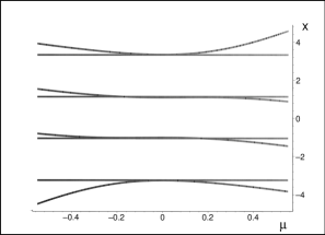
Figure 1: The quality of approximation of the $\mu-$independent spectrum of $\hat{Q}^{(4)}$ by the $\mu-$dependent grid-point eigenvalues of the Hermitian position matrix $\hat{q}^{(4)}(\mu)$ considered in the leading-order tridiagonal small$-\mu$ approximation (16).

The consistency of the perturbation calculations with respect to the small ${\mu}$ may be reconfirmed by the inspection of Figure 2 in which one sees that the smallest eigenvalue of the exact one-parametric $\alpha=1$ (i.e., tridiagonal) metric (15) ceases to be positive at the not too large values of $|{\mu}|\approx 0.3$. The exact formula

$$\Theta_{1}^{(4)}({\mu})>0\ \ {\rm iff}\ \ {\mu}\in\ \left(-{\mu}_{0},{\mu}_{0}\right)\,,$$

$${\mu}_{0}=1/\sqrt{6+2\,\sqrt{6}}\approx 0.3029054464$$ (17)

is also available due to the exact solvability of the model at $N=4$.

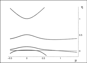
Figure 2: The ${\mu}-$dependence of the quadruplet of the eigenvalues of the tridiagonal candidate (15) for the metric.

4.3 Two-parametric pentadiagonal metric

Our above commentary accompanying Figure 2 means that at the larger $\mu$ the requirement of the positivity of the metric can only be satisfied at $\alpha\geq 2$, i.e., in a less trivial physical domain ${\cal D}$ of the available variable parameters $k$, ${\mu}$, $p$ and $d$ entering the fully general formula of Eq. (15) for the metric.

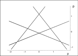
Figure 3: The boundaries of the domain of positivity of the pentadiagonal candidate for the metric.

The simplicity of our $N=4$ model enables us to make this argument more quantitative. The explicit $\alpha=2$ choice of the two variable parameters $\mu$ and $p$ in the metric

$$\Theta_{2}^{(4)}({\mu},p)=\left[\begin{array}[]{cccc}1&{\mu}&p&0\\ \vskip 6.0pt plus 2.0pt minus 2.0pt\cr{\mu}&1/2+2\,p&1/2\,{\mu}&1/2\,p\\ \vskip 6.0pt plus 2.0pt minus 2.0pt\cr p&1/2\,{\mu}&p+1/8&1/8\,{\mu}\\ \vskip 6.0pt plus 2.0pt minus 2.0pt\cr 0&1/2\,p&1/8\,{\mu}&1/12\,p+1/48\end{array}\right]$$

can be used for this purpose. In a preliminary graphical analysis we reveal (cf. Figure 3) that the two-dimensional version of the physical domain ${\cal D}$ has the piecewise linear boundaries. A more rigorous explanation can be also provided since the boundary lines may be identified with the loci of zeros of the secular polynomial $S({\mu},p,\eta)=\det(\Theta_{2}^{(4)}({\mu},p)-\eta)$ at $\eta=0$. Once we evaluate

$$S({\mu},p,0)=\det\Theta_{2}^{(4)}({\mu},p)=$$

$$={\frac{1}{768}}-1/8\,{p}^{2}{{\mu}}^{2}-1/6\,{p}^{3}+1/16\,{p}^{2}+1/12\,{p}^{4}+1/48\,p-{\frac{1}{64}}\,{{\mu}}^{2}+{\frac{1}{64}}\,{{\mu}}^{4}$$

we reveal that the polynomial $S({\mu},p,0)$ factorizes. This explains the existence of the two left-right symmetric pairs of the straight nodal lines which cross at ${\mu}=0$. The upper one is prescribed by the equation

$${\mu}_{upper}\sim\pm(p-p_{upper})=\pm\left(p-{\frac{1}{2\,\sqrt{6}-4}}\right)$$

(in Fig. 3, this is the upper pair crossing at the positive, maximal admissible $p_{upper}=1.112372435$). Similarly, the lower pair of lines given by the equation

$${\mu}_{lower}\sim\pm(p-p_{lower})=\pm\left(p+{\frac{1}{2\,\sqrt{6}+4}}\right)$$

crosses at the minimal, negative $p_{lower}=-0.1123724357$.

Along the line $p=0$, Fig. 3 correctly reproduces the position of the two boundaries (17) of the interval of the positivity of all of the eigenvalues of $\Theta_{1}^{(4)}({\mu})$ as displayed in Fig. 2. The same picture also explains why this interval of positivity of the metric grows with $p>0$ up to $p_{maximal}=1$.

5 Summary

In accord with all textbooks on quantum mechanics the set of the operators of observables (sampled here by the position $\mathfrak{q}$ and energy $\mathfrak{h}$) must be kept Hermitian in a certain physical Hilbert space of states (here, in ${\cal H}^{(P)}$). In such a setting the starting idea of our present paper was that such a Hilbert space may be replaced by any unitarily equivalent alternative (in our notation, by ${\cal H}^{(S)}$).

The majority of the existing applications of such an idea is built upon the unitary, Fourier-like correspondence ${\cal F}$ between bra or ket elements of the two spaces. In our present paper we rather made use of an indirect, manifestly non-unitary correspondence $\Omega$ involving just the ket vectors of the two spaces [8]. As far as we know (cf. also several additional comments collected in Appendix B), the first use of such a correspondence (called Dyson map) found its applications in nuclear physics [10].

Our present form of Hilbert spaces ${\cal H}^{(P)}$ or ${\cal H}^{(S)}$ has been chosen finite-dimensional, generated via a systematic $N-$point discretization of the real line of coordinates. The underlying idea was that in such a setting the efficiency of the calculations need not necessarily be optimal when we diagonalize, by brute force, all of the matrices in question (i.e., here, the pair of matrices $\mathfrak{q}$ and $\mathfrak{h}$). We imagined that even the Hermiticity of the matrices of observables need not be a condition sine qua non. We argued that the non-diagonal forms of these matrices, whenever sufficiently compact, would offer a way towards a minimization of the time needed for the numerical evaluations of phenomenological predictions.

For illustrative purposes we started from the choice of the “kinematic” grid-point eigenvalues $x_{j}^{(HP)}$ of a matrix $\mathfrak{q}$. We imagined that the latter matrix may be further simplified via a nonunitary Fourier-like transformation $\Omega^{-1}$,

$${\cal H}^{(P)}\ \longrightarrow\ {\cal H}^{(F)}\,.$$ (18)

In the latter, naively chosen Hilbert space the isospectral analogue $\hat{Q}$ of the position appears non-Hermitian but the remedy is easy. In the subsequent “Hermitization” step

$${\cal H}^{(F)}\ \longrightarrow\ {\cal H}^{(S)}\,$$ (19)

one simply endows the old space with a new, nontrivial metric $\Theta\neq I$, i.e., with an alternative, amended inner product.

Our present attention has been paid to the definition of the third space ${\cal H}^{(S)}$. We showed that and how the trick (18) plus (19) opens a new paradigm in the constructive analysis of quantum dynamics by making the pullback $\hat{Q}\ \longrightarrow\ \mathfrak{q}$ internally consistent. We showed that even though our pre-selected operators $\mathfrak{q}$ or $\hat{Q}$ of the coordinate were not diagonal, their respective Hermiticity inside ${\cal H}^{(P)}$ and ${\cal H}^{(S)}$ has still been, constructively, guaranteed.

On such a purely kinematical background the alternative dynamics were assumed given by the variable class of energy observables $\mathfrak{h}$. We explained how these Hamiltonian matrices may be related to their cryptohermitian avatars $H$, and how their eigenfunctions might be assigned the standard probabilistic interpretation. Thus, in contrast to the existing literature as reviewed, say, in [11] and starting from the wave functions in $x-$representation, we did not postulate any Hamiltonian in advance. We merely fixed its eligible class compatible with the pre-selected, smeared-coordinate representation of the wave functions.

Our main emphasis has been put on a minimal smearing of the position. For the entirely pragmatic purposes we selected the $N-$plet of grid points $x_{j}$ adapted to the optimal precision of the (discrete, approximate) integrations. Our matrices $\hat{Q}^{(N)}$ have been chosen tridiagonal, representing just one of the most elementary lattice grids given as the Hermite-polynomial zeros. We expect that such a strategy will optimize the precision of approximants, especially when evaluating or prescribing the norms and/or inner products of wave functions.

Summarizing, we proposed here the kinematical choice of the cryptohermitian position $\hat{Q}^{(N)}$ accompanied by the dynamics-determining specification of one of the eligible metrics $\Theta_{\alpha}$. In such a framework we indicated the possibility of varying the dynamics and/or of moving towards a systematic and exhaustive construction and classification of all of the alternative, $\alpha-$numbered physical Hilbert spaces, be it ${\cal H}^{(P)}_{\alpha}$ and/or its unitary equivalent, less usual version ${\cal H}^{(S)}_{\alpha}$ with nontrivial metrics given, in our illustrative example, in closed form.

Appendix A: A comment on choices of grid points

One of the roots of the popularity of the representation of the quantum-state ket-vectors $|\psi\rangle$ in their wave-function (alias “coordinate-representation”) form $\psi(x)\in L^{2}(\mathbb{R},\mu)$ may be seen in the user-friendliness of the formula giving their norm,

$$\|\psi\|:=\sqrt{\int_{-\infty}^{\infty}\,\psi^{*}(x)\psi(x){\omega}(x)dx}\,.$$ (20)

In a way similar to the definition of the Hilbert-space inner product

$$\langle\psi|\phi\rangle:=\int_{-\infty}^{\infty}\,\psi^{*}(x)\phi(x){\omega}(x)dx\,$$

these integrals contain a weighting function ${\omega}(x)$ which is most often set equal to a constant or a power of $x$ or a Gaussian.

The necessity of the evaluation of these integrals is ubiquitous. Its precision represents one of the limiting factors of the practical applicability of the theory. In particular, various empirical tests are very often passed by the so called Gauss-Hermite quadrature [5]

$$\int_{-\infty}^{\infty}\,e^{-x^{2}}\,f(x)\,dx\ =\sum_{j=0}^{N-1}\,w_{j}\,f(x_{j})+error[N,f^{(2N)}(\xi)]\,.$$ (21)

In such a Gaussian-weighted approximative formula the size of the error term is very often found acceptably small over the relevant class of the integrands. Its grid-point quantities $x_{j}$ are identified with the the roots of the well known Hermite polynomials (this identification is sampled by our present Eq. (3) above). The necessary weight factors are also obtainable in compact form, $w_{j}=w_{j}^{(N)}=C(N)/[H(N-1,x_{j})]^{2}$. The more detailed information (i.e., the proportionality factor $C(N)$, etc) may be found not only in standard monographs [12] but also, directly and free of charge, via web [13, 14].

Appendix B: A comment on the concept of cryptohermiticity

In the Dieudonné’s paper [9] operators $\hat{Q}$ satisfying relation (12) at a suitable positive and self-adjoint “metric” $\Theta$ were studied and given the name of “quasi-Hermitian” operators, $\hat{Q}\in{\cal L}^{(QH)}$. In their full generality and without additional assumptions, they were emphasized to exhibit peculiar and strongly counterintuitive, truly “non-Hermitian” properties. In particular, once they were not assumed to be Riesz operators or compact symmetrizable operators, their spectrum was shown not to be necessarily real. Moreover, their adjoints were shown non-quasi-Hermitian in general, $\hat{Q}^{\dagger}\notin{\cal L}^{(QH)}$.

In the historical perspective it may be considered rather unfortunate that more than thirty years later, Scholtz, Geyer and Hahne [10] decided to choose, incidentally, the same name for the well-behaved and very narrow compact-operator subset ${\cal L}^{(SGH)}$ of the Dieudonné’s quasi-Hermitian set. This is the reason why we use here the terminology inspired by Smilga [15] and why we call the elements of the set ${\cal L}^{(SGH)}$ cryptohermitian operators.

The most natural and physics-motivated extension of the cryptohermitian class ${\cal L}^{(SGH)}$ is the Mostafazadeh’s [16] set of the so called “pseudo-Hermitian” operators ${\cal L}^{(PH)}$ for which, roughly speaking, all of the invertible and self-adjoint operators $\Theta$ compatible with Eq. (12) (and denoted, therefore, by another symbol, say, ${\cal P}$) may remain indefinite. A potentially equivalent name of ${\cal PT}-$symmetric operators is usually reserved, by its proponents [17, 18, 19], to the narrower class of models where ${\cal P}$ coincides with the operator of parity and where it may be interpreted as the indefinite metric in Krein space [20].

One of the most compact approaches to the applications of ${\cal PT}-$symmetric operators in quantum theory has been reviewed by Carl Bender [11]. He considers merely the intersection of the cryptohermitian and ${\cal PT}-$symmetric classes of operators of potential observables while picking up a unique metric in the product form $\Theta^{(CB)}={\cal PC}$. The key merit of this approach is that the factor ${\cal C}$ with the property ${\cal C}^{2}=I$ may be interpreted as a charge of the system. The alternative name for ${\cal C}$ as proposed in [21] (viz., “quasiparity”) has not been given the meaning of an observable and found much less users in the literature, therefore [22].

References

- [1] J. Hilgevoord, Am. J. Phys. 70 (2002) 301.
- [2] M. Znojil, Int. J. Theor. Phys. 50 (2011) 1052.
- [3] M. Znojil, J. Phys. A: Math. Gen. 30 (1997) 8771.
- [4] for a characteristic sample of usage in molecular physics and chemistry cf., e.g., the MOLPRO software package http://www.molpro.net/, maintained by H.-J. Werner and P. J. Knowles.
- [5] M. Abramowitz and I. A. Stegun, Handbook of Mathematical Functions (Dover, New York, 1970).
- [6] Frank W. J. Olver, Daniel W. Lozier, Ronald F. Boisvert, Charles W. Clark, Eds., NIST Handbook of Mathematical Functions (Cambridge University Press, Cambridge, 2010).
- [7] B. W. Char et al, Maple V Language Reference Manual (Springer, New York, 1993).
- [8] M. Znojil, SYMMETRY, INTEGRABILITY and GEOMETRY: METHODS and APPLICATIONS 5 (2009) 001.
- [9] J. Dieudonne, Proc. Int. Symp. Lin. Spaces (Pergamon, Oxford, 1961), p. 115.
- [10] F. G. Scholtz, H. B. Geyer and F. J. W. Hahne, Ann. Phys. (NY) 213 (1992) 74.
- [11] C. M. Bender, Rep. Prog. Phys. 70 (2007) 947; A. Mostafazadeh, Int. J. Geom. Meth. Mod. Phys. 7 (2010) 1191.
- [12] J. Stoer and R. Bulirsch. Introduction to Numerical Analysis (Springer-Verlag, New York, 1980).
- [13] For tables of Gauss-Hermite abscissae and weights up to order n = 32 see http://www.efunda.com/math/num_integration/findgausshermite.cfm.
- [14] NIST Digital Library of Mathematical Functions: http://dlmf.nist.gov/
- [15] A. V. Smilga, J. Phys. A: Math. Theor. 41 (2008) 244026.
- [16] A. Mostafazadeh, J. Math. Phys. 43 (2002) 205, 2814 and 3944.
- [17] D. Bessis, private communication, 1992; J. Zinn-Justin, private communication, 2010.
- [18] V. Buslaev and V. Grecchi, J. Phys. A: Math. Gen. 26 (1993) 5541.
- [19] C. M. Bender and S. Boettcher, Phys. Rev. Lett. 80 (1998) 5243.
- [20] H. Langer and Ch. Tretter, Czechosl. J. Phys. 54 (2004) 1113.
- [21] M. Znojil, arXiv:math-ph/0104012.
- [22] G. Lévai, Czechosl. J. Phys. 54 (2004) 77; A. Sinha and P. Roy, Czechosl. J. Phys. 54 (2004) 129; O. Mustafa, Int. J. Theor. Phys. 47 (2008) 1300.