Negative thermal conductivity of chains of rotors with mechanical forcing

Abstract

We consider chains of rotors subjected to both thermal and mechanical forcings, in a nonequilibrium steady-state. Unusual nonlinear profiles of temperature and velocities are observed in the system. In particular, the temperature is maximal in the center, which is an indication of the nonlocal behavior of the system. Despite this uncommon behavior, local equilibrium holds for long enough chains. Our numerical results also show that, when the mechanical forcing is strong enough, the energy current can be increased by an inverse temperature gradient. This counterintuitive result again reveals the complexity of nonequilibrium states.

I Introduction

Thermodynamic properties of non-equilibrium stationary states are poorly understood. They are usually characterized by currents of conserved quantities, such as energy, flowing through the system. When stationary states are close to equilibrium states, linear response theory is effective and explains common macroscopic phenomena like Fourier’s law: In a system in contact with two thermostats at different temperatures, the heat flux is proportional to the temperature gradient (as long as the relative difference between the two temperatures is small).

In contrast, there is no general theory to describe systems in a stationary state far from equilibrium, and the corresponding macroscopic properties seem to depend on the specific details of the dynamics.

In this article, we investigate numerically the energy transport properties of a simple one-dimensional system, a chain of $N$ rotors, in a stationary state far from equilibrium. Many studies considered one-dimensional chains of oscillators subjected to a temperature gradient Lepri et al. (2003); Dhar (2008). Here we consider both thermal and mechanical forcings, obtained as follows: The leftmost rotor is attached to a wall and put in contact with a Langevin thermostat at temperature $T_{\rm L}$, while the rightmost rotor is subjected to a constant external force $F$ and put in contact with another Langevin thermostat at temperature $T_{\rm R}$.

What we observe in our numerical experiments is that the combined effect of these two generalized forces can reduce the current instead of increasing it. This counterintuitive effect is observed for large mechanical forcings $F$, when $T_{\rm R}$ is increased while $T_{\rm L}$ remains fixed (see Figure 8 below). The mechanical forcing induces a negative current (from the right to the left). When $T_{\rm R}$ is increased while $T_{\rm L}$ remains fixed, one would naively expect that the (negative) thermal forcing is also larger, and thus that the negative current should be (in absolute value) larger. In contrast to this expectation, we observe that, in this case, the current is reduced. This strange effect does not appear if, instead, $T_{\rm L}$ is lowered and $T_{\rm R}$ is fixed (see Figure 6 below), in which case the current indeed becomes larger in absolute value.

We are unable to provide explanations to the above described phenomena. We believe that such behaviors show the complexity of non-equilibrium stationary states far from equilibrium, and also suggest that Fourier’s law is only valid close to equilibrium. A naive extension of the definition of thermal conductivity to genuinely non-equilibrium settings can give negative values to this quantity (whence the somehow provocative title of this article).

In the sequel of this article, we first describe the system we work with, and the numerical integrator we have used (see Sec. II). We next turn to studying various properties of the system. In particular, we numerically check that local equilibrium holds for systems large enough, despite the fact that, globally, the system is out of equilibrium (see Sec. III.2). In Sec. III.3, we study how the current depends on the magnitude of the mechanical force and on the temperatures that are imposed on both ends of the chain. All these numerical studies are performed for chains of increasing lengths.

II Description of the system

The configuration of the system is described by the positions (angles) $q=(q_{1},\dots,q_{N})$ of the rotors, which belong to the one-dimensional torus $2\pi\mathbb{T}$, as well as their associated (angular) momenta $p=(p_{1},\dots,p_{N})$. The masses of the particles are set to 1 for simplicity. The Hamiltonian of the system is

$$H(q,p)=\sum_{i=1}^{N}\left[\frac{p_{i}^{2}}{2}+(1-\cos r_{i})\right],$$ (1)

where we have set $r_{i}=q_{i}-q_{i-1}$ for $i\geq 2$ and $r_{1}=q_{1}$.

We consider a system with free boundary conditions on the right end, whose evolution equations read:

$$\left\{\begin{aligned} dq_{i}&=p_{i}\,dt,\\ dp_{i}&=\Big{(}\sin(q_{i+1}-q_{i})-\sin(q_{i}-q_{i-1})\Big{)}dt,\ i\neq 1,N,\\ dp_{1}&=\Big{(}\sin(q_{2}-q_{1})-\sin(q_{1})\Big{)}dt\\ &\qquad\qquad-\gamma p_{1}\,dt+\sqrt{2\gamma T_{\rm L}}\,dW^{1}_{t},\\ dp_{N}&=\Big{(}F-\sin(q_{N}-q_{N-1})\Big{)}dt\\ &\qquad\qquad-\gamma p_{N}\,dt+\sqrt{2\gamma T_{\rm R}}\,dW^{N}_{t},\\ \end{aligned}\right.$$ (2)

where $W^{1}_{t}$ and $W^{N}_{t}$ are independent standard Wiener processes, and $\gamma>0$ determines the strength of the coupling to the thermostat. In the sequel, we work with $\gamma=1$. Note that the external constant force $F$ is non-gradient since it does not derive from a periodic potential.

We checked the robustness of the results we describe below with respect to the choice of boundary conditions. We indeed also considered fixed boundary conditions on the right end (this amounts to adding an extra force $-\sin(q_{N})$ to the last atom). In particular, we checked that our counterintuitive results on the behavior of the thermal current as a function of the strength of the nongradient force are still observed with these boundary conditions.

II.1 Equilibrium and nonequilibrium states

If $F=0$ and $T_{\rm L}=T_{\rm R}=T$, the system is in equilibrium, and the unique stationary measure is given by the Gibbs measure at temperature $T$ associated with the Hamiltonian (1). When $T_{\rm L}\neq T_{\rm R}$ with $F=0$, the properties of the non-equilibrium stationary state have been studied numerically by various authors Giardiná et al. (2000); Gendelman and Savin (2000); Yang and Hu (2005); Gendelman and Savin (2005). The thermal conductivity of the system, defined as the stationary energy current multiplied by the size of the system and divided by the temperature difference Bonetto et al. (2000), has a finite limit for large system sizes, even though the rotor chain is a momentum conserving one-dimensional system Basile et al. (2006, 2009). Besides, as the average temperature $T$ increases above the value 0.5, the thermal conductivity decreases dramatically Giardiná et al. (2000).

If $F\neq 0$, the system is out-of-equilibrium even if $T_{\rm L}=T_{\rm R}$ (recall indeed that $F$ is non-gradient). The force, in the stationary state, induces an energy current towards the left. The stationary state cannot be computed explicitly and, if $F$ is large, linear response theory cannot be used to obtain information about the conductivity of the system.

If $T_{\rm L}<T_{\rm R}$, there are two mechanisms that separately generate an energy current towards the left of the system: The mechanical force $F$ and the thermal force given by the temperature gradient. It seems however difficult to separate the contributions of each mechanism. The numerical experiments reported below show that these two mechanisms are not necessarily additive, and that one mechanism may reduce the effect of the other one, leading to counterintuitive results.

II.2 Numerical integration

The numerical integration of (2) is performed using a splitting strategy where the Hamiltonian part of the evolution is integrated with the Verlet scheme Verlet (1967). The fluctuation-dissipation parts, with the additional non-gradient force, are Ornstein-Uhlenbeck processes and can thus be integrated analytically. We have thus used the following algorithm:

$$\widetilde{p}^{n}_{1} = \alpha p^{n}_{1}+\sigma_{\rm L}G^{n}_{1},$$

$$\widetilde{p}^{n}_{N} = F+\alpha(p^{n}_{N}-F)+\sigma_{\rm R}G^{n}_{N},$$

$$\widetilde{p}^{n}_{i} = p^{n}_{i},\quad i\neq 1,N,$$

$$p^{n+1/2}_{i} = \widetilde{p}^{n}_{i}-\frac{\Delta t}{2}\frac{\partial H}{\partial q_{i}}(q^{n},\widetilde{p}^{n}),$$

$$q^{n+1}_{i} = q^{n}_{i}+\Delta t\,p^{n+1/2}_{i},$$

$$p^{n+1}_{i} = p^{n+1/2}_{i}-\frac{\Delta t}{2}\frac{\partial H}{\partial q_{i}}(q^{n+1},p^{n+1/2}),$$

where $\alpha=\exp(-\gamma\Delta t)$, $\displaystyle\sigma_{\rm L}=\sqrt{(1-\alpha^{2})T_{\rm L}}$, $\displaystyle\sigma_{\rm R}=\sqrt{(1-\alpha^{2})T_{\rm R}}$, and $H$ is given by (1). In turn, $G^{n}_{1}$ and $G^{n}_{N}$ are independent normal Gaussian random variables. Recall also that the friction parameter $\gamma$ is set to 1. The three first lines of the above algorithm consist in exactly integrating the Ornstein-Uhlenbeck processes on $p_{1}$ and $p_{N}$, whereas the three last lines are based on the standard Verlet algorithm.

The time-step $\Delta t=0.05$ ensures that the energy conservation in the Verlet scheme is accurate enough. While there might be some time-step bias in the value of the currents, the qualitative conclusions are robust with respect to the choice of the time-step.

III Properties of the nonequilibrium system

This section is organized as follows. First, we discuss the existence of a stationary measure for the dynamics (2). Under the assumption that such a stationary measure exists, we establish some relations that are consistent with physical intuition. We next point out that this system shows some very surprising features. For instance, the temperature profile is non-monotonic and a maximum is observed in the center of the system, while the velocity profiles are very nonlinear. Despite these nonlocal features, we show that local equilibrium holds. We finally turn to investigating the dependence of the stationary energy current on $F$, $T_{\rm L}$ and $T_{\rm R}$.

III.1 Stationary measure

We believe that there exists a unique smooth stationary measure for the dynamics (2). However, as far as we know, there is no rigorous result in this direction for rotor chains, even in the case $F=0$. Indeed, the standard techniques (see for instance Rey-Bellet (2006); Carmona (2007)) used to prove existence and uniqueness of an invariant measure for chains of oscillators under thermal forcing do not apply here.

A possible pathology for rotor chains is that the (internal) energy concentrates locally on one or several rotors, which rotate faster and faster. Since the interaction forces are bounded, it may not be possible to prevent this fast rotation. In practice, we have not observed such catastrophes in the parameter regime we considered, but the kinetic temperature profiles presented in Figure 1 (obtained from the variance of the momenta, with the previously mentioned caveat on the interpretation of this quantity) are quite unexpected and show that the internal energy tends to be larger in the middle of the chain. This picture also allows to understand what happens when the imposed temperatures at the right and left ends change: The maximal temperature in the chain is almost unchanged, but the position of the maximum is displaced. This shows that the linear response correction to the stationary measure is necessarily nonlocal. Such nonlocal effects were already observed in nonequilibrium exclusion processes Derrida et al. (2002a, b).

Figure 1: Kinetic temperature profiles for chains of length $N=1024$, with $F=1.6$ and different temperature gradients.

Some interesting relations can nonetheless be obtained under the assumption that the stationary state exists. We denote by $\langle\cdot\rangle$ the expectation with respect to the stationary measure. First, a constant profile of force settles down in the bulk. Taking expectations in (2) indeed gives

$$\langle\sin r_{i+1}\rangle =\langle\sin r_{i}\rangle,\qquad\qquad\qquad i\neq 1,N,$$

$$\langle\sin r_{2}\rangle =\langle\sin r_{1}\rangle+\gamma\langle p_{1}\rangle,$$

$$\langle\sin r_{N}\rangle =F-\gamma\langle p_{N}\rangle.$$

This leads to the following profile: $F_{i}:=\langle\sin r_{i}\rangle=F-\gamma\langle p_{N}\rangle$ for all $i\geq 2$, while $F_{1}:=\langle\sin r_{1}\rangle=F-\gamma(\langle p_{N}\rangle+\langle p_{1}\rangle)$.

The balance between the average work done by the force and the energy dissipated by the thermostats is given by

$$0=F\langle p_{N}\rangle+\gamma(T_{\rm L}-\langle p_{1}^{2}\rangle)+\gamma(T_{\rm R}-\langle p_{N}^{2}\rangle),$$ (3)

as can be seen by noticing that the average variation of the total energy $H$ is zero. Moreover, the entropy production inequality (obtained by computing the variations of the relative entropy with respect to the invariant measure, see e.g. Bernardin and Olla (2011)) gives

$$T_{\rm L}^{-1}(T_{\rm L}-\langle p_{1}^{2}\rangle)+T_{\rm R}^{-1}(T_{\rm R}-\langle p_{N}^{2}\rangle)\leq 0.$$

In the case $T_{\rm L}=T_{\rm R}=T$, this relation, combined with (3), yields $F\langle p_{N}\rangle\geq 0$. Therefore the stationary momentum on the right end has the same sign as the driving force, as expected.

Figure 2 shows that the momentum profile is not linear, and that its derivative is maximal where, according to Figure 1, temperature is maximal. We also observe on Figure 3 (top) that the profile seems to become steeper in the thermodynamic limit.

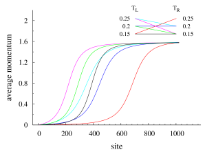
Figure 2: Average momenta for chains of length $N=1024$, with $F=1.6$.

III.2 Local equilibrium and thermodynamic limit

A very interesting question is whether nonequilibrium systems are locally close to equilibrium. This issue was considered in Mai et al. (2007) for systems subjected to thermal forcings only. We check the local equilibrium assumption in three steps.

1. We study the agreement between the local kinetic temperature (defined as the variance of the velocities) and the local potential temperature. The latter is obtained as follows. First, we numerically precompute the function

   $$g:T\mapsto\frac{\displaystyle\int_{0}^{2\pi}V(r)\exp(-V(r)/T)\,dr}{\displaystyle\int_{0}^{2\pi}\exp(-V(r)/T)\,dr}$$

   which, to a given temperature, associates the canonical average of the potential energy $V(r)=1-\cos r$ of one bond. The local potential temperature at bond $i$ is then defined as the value $T_{i}$ such that $g(T_{i})$ is equal to the time average of the potential energy of the bond $r_{i}$ along the trajectory defined by (2). The results presented in Figure 3 (bottom) show that the two local temperatures are quite different for small systems, but are identical for larger ones. Besides, as the length of the system increases, the profiles become more symmetric.

   

   

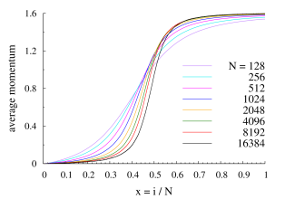
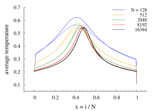
   Figure 3: Rescaled profiles for systems of increasing size $N=2^{k}$ with $k=7,\dots,14$: the $x$ variable is the site index $i$ divided by $N$. The value of the nongradient force is $F=1.6$ and $T_{\rm L}=T_{\rm R}=0.2$. Top: momenta. Bottom: kinetic (solid lines) and potential (dashed lines) temperatures.

2. We check that the individual distributions of $p$ and $r$ are in accordance with a local Gibbs equilibrium. To this end, we build the histograms of the momenta and distances at the site $i_{\rm max}$ where the local temperature is maximal (since this is the location where the disagreement between the local kinetic and potential temperatures is the strongest). The results presented in Figure 4 show that the empirical distributions of $p$ and $r$ at the site $i_{\rm max}$ are in excellent agreement with the Gibbs distributions with the same parameters (average velocity $\overline{p}_{i}$, temperature $T_{i}$), namely

   $$Z_{\rm kin}^{-1}\exp\left[-(p-\overline{p}_{i})^{2}/(2T_{i})\right]\,dp$$

   and

   $$Z_{\rm pot}^{-1}\exp\left[-V(r)/T_{i}\right]\,dr,$$

   except for the smallest systems (say, $N\leq 512$).

   \psfrag{momenta}{momentum}\psfrag{distances}{distance}\includegraphics[width=170.71652pt,angle={-90}]{Plots/figHistP.eps}

   \psfrag{momenta}{momentum}\psfrag{distances}{distance}\includegraphics[width=199.16928pt]{Plots/figHistR.eps}

   Figure 4: Top: Empirical distribution of momenta at the site $i_{\rm max}$ (where the temperature is maximal), and comparison with the local Gibbs equilibrium with the same average and variance. Bottom: Empirical distribution of the distances at bond $i_{\rm max}$ and comparison with the local Gibbs equilibrium with the same average energy. Both plots correspond to a chain of length $N=1024$, with $F=1.6$ and $T_{\rm L}=T_{\rm R}=0.2$.

3. We check that momenta and distances are independent. To this end, we compare the joint law $\psi=\psi(r_{i_{\rm max}},p_{i_{\rm max}})$ of $(r_{i_{\rm max}},p_{i_{\rm max}})$ and the product law obtained from the tensor product of the individual distributions of these two variables (denoted respectively by $\overline{\psi}_{r}(r_{i_{\rm max}})$ and $\overline{\psi}_{p}(p_{i_{\rm max}})$). More precisely, for a given number $n$ of sample points (obtained by subsampling a long trajectory every $10^{4}$ steps), we check that the distance

   $$\delta_{n}=\int_{[0,2\pi]\times\mathbb{R}}\left|\psi^{n}(r,p)-\overline{\psi}^{n}_{r}(r)\overline{\psi}^{n}_{p}(p)\right|\,dr\,dp$$ (4)

   between these two distributions indeed decreases as the inverse square-root of the number of configurations used to build the histograms. Again, this is true for systems large enough. Figure 5 shows that $\delta_{n}\sim n^{-1/2}$.

   \psfrag{chain length}{$\log_{2}n$}\psfrag{joint error}{$\log_{2}\delta_{n}$}\includegraphics[width=227.62204pt]{Plots/figJointErr.eps}

   Figure 5: Decrease of the error $\delta_{n}$ defined by (4) as a function of the number of sample points $n$. Estimated rate of decrease: $\delta_{n}\simeq 28.7\times n^{-0.494}$.

III.3 Behavior of the energy current

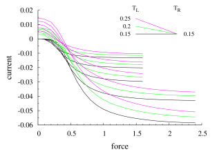
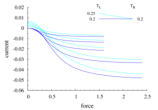
Figure 6: Comparison of the currents with fixed temperature on the right end and increasing temperatures on the left end. From top to bottom: decreasing system sizes $N=2048,1024,512,256,128$ (the ordering is the same for all situations considered; for the longest systems, we have considered forces $0\leq F\leq 1.6$; for the shortest ones, we have considered the range $F\in[0;2.4]$).

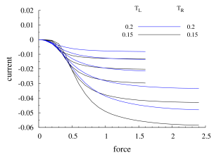
Figure 7: Comparison of the currents with fixed temperature difference. From top to bottom: decreasing system sizes $N=2048,1024,512,256,128$ (the ordering is the same for all situations considered).

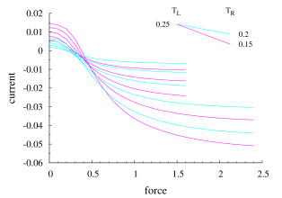
Figure 8: Comparison of the currents for a fixed temperature at the left end and various temperature differences. From top to bottom: decreasing system sizes $N=2048,1024,512,256,128$ (the ordering is the same for all situations considered).

We consider the following situations:

1. same temperatures on the left and on the right: $(T_{\rm L},T_{\rm R})=(0.20,0.20)$ or $(0.15,0.15)$;

2. hot left end and cold right end: $(T_{\rm L},T_{\rm R})=(0.25,0.15)$, $(0.20,0.15)$ or $(0.25,0.20)$;

3. cold left end and hot right end: $(T_{\rm L},T_{\rm R})=(0.15,0.25)$.

Currents are computed as a function of the magnitude $F$ of the non-gradient forcing term for systems of different lengths: $N=128$, 256, 512, 1024, 2048. Recall that local equilibrium holds at the leading order, so that the energy current is induced by the first order corrections in $1/N$.

We first compare the currents when the temperature on the right end is fixed (see Figure 6). As expected, the negative current induced by the mechanical forcing is reduced by the opposite, positive thermal current.

We next compare the currents at fixed temperature difference $T_{\rm R}-T_{\rm L}$, for different average temperatures (see Figure 7). In this case, we observe that, for strong mechanical forcings, the current is enhanced when the average temperature decreases, while the opposite happens when the mechanical forcing is small.

We finally turn to the most interesting situation. The temperature on the left end is fixed and the temperature on the right end varies (see Figure 8). In this case, counterintuitive results are observed for large mechanical forcings: The total current is enhanced as $T_{\rm R}$ decreases, even though, in such a situation, the thermal gradient is in the opposite direction. The mechanical forcing induces a negative current, while the thermal gradient induces (in the absence of any force) a positive current. The combined effect of both mechanical and thermal forcings induces a negative current larger (in absolute value) than the one in the absence of any thermal gradient!

IV Discussion of the results

In conclusion, for large mechanical forcings $F$, we observe that

1. when $T_{\rm R}$ is fixed, the current varies qualitatively as when there is no mechanical forcing: The absolute value of the current increases when $T_{\rm L}$ decreases, which means that the current induced by the thermal forcing and the current induced by the mechanical forcing are somewhat additive. In this case, a positive thermal conductivity is observed (for a fixed value $F$ of the mechanical forcing, considering only the response in the limit when $T_{\rm R}-T_{\rm L}\to 0$).

2. when $T_{\rm L}$ is fixed, the current has a surprising behavior: Its absolute value increases when $T_{\rm R}$ decreases. This means that the thermal forcing, which is naively expected to reduce the current induced by the mechanical forcing, actually enhances it. In this case, a negative thermal conductivity is observed (again, for a fixed value $F$ of the mechanical forcing).

A possible interpretation is based on the fact that, for such a system, the thermal conductivity is a decreasing function of the temperature when $F$ is large (see Figure 7). It is possible that, by lowering $T_{\rm R}$ and thus increasing the conductivity at the right end, one makes the system more sensitive to the mechanical forcing. The increased mechanical current may hence counterbalance the increased opposite thermal current.

An interesting question which we did not discuss here is the scaling of the energy current as a function of the system size when $F\neq 0$. Some preliminary results suggest that the thermal conductivity is finite, as when $F=0$, but this question definitely calls for additional studies.

References

Lepri et al. (2003)
S. Lepri,
R. Livi, and
A. Politi,
Phys. Rep. 377,
1 (2003).
Dhar (2008)
A. Dhar, Adv.
Phys. 57, 457
(2008).
Giardiná et al. (2000)
C. Giardiná,
R. Livi,
A. Politi, and
M. Vassalli,
Phys. Rev. Lett. 84,
2144 (2000).
Gendelman and Savin (2000)
O. V. Gendelman
and A. V. Savin,
Phys. Rev. Lett. 84,
2381 (2000).
Yang and Hu (2005)
L. Yang and
B. Hu, Phys.
Rev. Lett. 94, 219404
(2005).
Gendelman and Savin (2005)
O. V. Gendelman
and A. V. Savin,
Phys. Rev. Lett. 94,
219405 (2005).
Bonetto et al. (2000)
F. Bonetto,
J. L. Lebowitz,
and
L. Rey-Bellet, in
Mathematical Physics 2000, edited by
A. Fokas,
A. Grigoryan,
T. Kibble, and
B. Zegarlinsky
(Imperial College Press, 2000), pp.
128–151.
Basile et al. (2006)
G. Basile,
C. Bernardin,
and S. Olla,
Phys. Rev. Lett. 96,
204303 (2006).
Basile et al. (2009)
G. Basile,
C. Bernardin,
and S. Olla,
Commun. Math. Phys. 287,
67 (2009).
Verlet (1967)
L. Verlet,
Phys. Rev. 159,
98 (1967).
Rey-Bellet (2006)
L. Rey-Bellet,
Lect. Notes Math. 1881,
41 (2006).
Carmona (2007)
P. Carmona,
Stoch. Proc. Appl. 117,
1076 (2007).
Derrida
et al. (2002a)
B. Derrida,
J. L. Lebowitz,
and E. R. Speer,
Phys. Rev. Lett. 89,
030601 (2002a).
Derrida
et al. (2002b)
B. Derrida,
J. L. Lebowitz,
and E. R. Speer,
J. Stat. Phys. 107,
599 (2002b).
Bernardin and Olla (2011)
C. Bernardin and
S. Olla,
arXiv cond-mat.stat-mech
(2011), eprint 1105.0493v1,
URL http://arxiv.org/abs/1105.0493v1.
Mai et al. (2007)
T. Mai,
A. Dhar, and
O. Narayan,
Phys. Rev. Lett. 98,
184301 (2007).