Series expansions from the corner transfer matrix renormalization group method: the hard squares model

Abstract

The corner transfer matrix renormalization group method is an efficient method for evaluating physical quantities in statistical mechanical models. It originates from Baxter’s corner transfer matrix equations and method, and was developed by Nishino and Okunishi in 1996. In this paper, we review and adapt this method, previously used for numerical calculations, to derive series expansions. We use this to calculate 92 terms of the partition function of the hard squares model. We also examine the claim that the method is subexponential in the number of generated terms and briefly analyse the resulting series.

Keywords: Corner transfer matrix, hard squares model, series expansions.

1 Introduction

In this paper, we adapt an efficient numerical method — the corner transfer matrix renormalization group, or CTMRG for short — for the purpose of generating series expansions for the properties of various statistical mechanical models.

Much work has been devoted in recent years to finding the most accurate (i.e. largest number of correct terms) series for a variety of models. One such model is the hard squares model. In this model, each spin can take the value 0 or 1, denoting an ‘empty’ or ’occupied’ site. The weight of a configuration is $z$ to the power of the number of 1 spins, and the hard squares constraint restricts the configurations so that no two 1 spins can be directly adjacent. We wish to find the partition function of the model,

$$Z_{N}=\sum_{\{\sigma_{i}\}}z^{\sum_{i}\sigma_{i}},$$

where the outside sum is over all valid configurations, and in particular the expansion in $z$ of the partition function per site:

$$\kappa=\lim_{N\rightarrow\infty}Z_{N}^{1/N}=1+z-2z+8z^{2}-40z^{3}+225z^{4}-\ldots$$

The current ‘state of the art’ for finding series expansions is the finite lattice method, pioneered by de Neef and Enting ([14, 13]) and subsequently developed and refined by Jensen, Guttmann, and Enting ([22, 23]). This method takes advantage of the fact that the infinite partition function series can be approximated up to a certain order by an expression involving the partition functions of several finite lattices.

By itself, the finite-lattice approximation to $\kappa$ is not particularly effective, but the method derives its power by using transfer matrices to calculate the partition function of the finite lattices. These are matrices, denoted by $V$ and indexed by the values of a column of spins, which contain the Boltzmann weight of a column, given the spins on the sides. Multiplication by $V$ ‘adds’ the weight of an extra column, so the partition function of the entire lattice can be built by repeating such multiplications. This can be used either to calculate the partition function of finite lattices, for the finite lattice method, or can be extended to the thermodynamic limit, where the partition function can be expressed as

$$Z=\lim_{N\rightarrow\infty}\mbox{Tr }V^{N}.$$

Therefore the partition function can be derived directly from the largest eigenvalue of the transfer matrix.

The CTMRG uses a similar concept of transfer matrices, but with a twist. Instead of containing the weight of a column, corner transfer matrices contain the weight of a full quarter of the lattice, given the spins at the boundaries. This means that the partition function is expressible as the sum of 4th powers of corner transfer matrices. The advantage of this representation is that approximating the ‘true’ infinite-dimensional matrices by finite-size matrices is often very accurate, even for small matrices. The disadvantage is that we must evaluate the full eigenvalue spectrum of the corner transfer matrices, rather than simply the largest eigenvalue.

The CTMRG method is quite general, and can in theory be applied to any model where the Boltzmann weight of a configuration can be expressed as the product of weights of a single cell. We call such models interaction round a face (IRF) models. In terms of such a model, the face weight of the hard squares model is given by

$$\omega\left(\begin{array}[]{cc}a&b\\ c&d\end{array}\right)=\left\{\begin{array}[]{rl}0&\mbox{if $a=b=1$, $a=c=1$, $b=d=1$ or $c=d=1$}\\ z^{(a+b+c+d)/4}&\mbox{otherwise.}\end{array}\right.$$

We note that the factor of $1/4$ comes from the fact that each spin lies in 4 cell faces.

The original corner transfer matrix method was developed by Baxter, Enting, and various co-authors starting from 1978. In [3], Baxter developed the corner transfer matrix equations, which underpin all CTM-related methods. We discuss these equations in detail below. He also developed the corner transfer matrix method, which involved transforming the CTM equations and iterating through them until a solution was reached.

This method was applied to the Ising model for low-temperature and high-field series expansions ([9, 16]), as well as the hard squares model ([10]). Using what would be considered today as insignificant computational power, they managed to extract a very large number of series terms for these models (in fact, we know of no longer series expansions for the hard squares model). More recently, Baxter used this method to numerically calculate the partition function for hard particle models at $z=1$ to high precision ([8]).

A notable triumph of the corner transfer matrix approach was Baxter’s exact solution of the hard hexagons model ([4]), which he derived by noticing a pattern in the eigenvalues of the corner transfer matrices. He was then able to prove the validity of this pattern and thus solve the model.

Other applications of this method by Baxter included the 8-vertex model ([1, 2]), the 3d Ising model for one-dimensional matrices ([11]), and the chiral Potts model ([5, 7, 6]). However, in each case the actual transformations applied were model-specific, so the method remained relatively limited in application.

In 1996, Nishino and Okunishi ([29, 35, 30]) used the CTM equations to derive the corner transfer matrix renormalization group method (CTMRG). This method calculates finite-size approximations to the solution of the CTM equations using a principle derived from the density matrix renormalization group method. Nishino and Okunishi applied this method numerically to various models — the $q=5$ Potts model ([32]), the 3d Ising model ([33]), and the spin-$\frac{3}{2}$ Ising model ([37]). They also converted it to 3-dimensional lattices in [31, 34, 28, 20], and studied the eigenvalue distribution of the CTM matrices in [36].

In 2003, Foster and Pinettes ([18, 17]) applied this method to the self-avoiding walk model, and more recently Mangazeev et al. ([26, 27]) used it to evaluate the scaling function of the Ising model in a magnetic field.

All of the above applications were for numerical calculations. As far as we know, no one has tried to use this method to derive series expansions. In principle, the method can be adapted to do this with no changes. However, in practice there are some implementational difficulties, notably that we must diagonalize a matrix of series. To our knowledge this has not been attempted before. These considerations give rise to some interesting mathematics and are the subject of this paper.

It is claimed (although not actually proved) that the method has complexity $O(\alpha^{\sqrt{n}})$, as opposed to the FLM which is an exponential-time method, albeit with a small growth constant. We will briefly examine this claim.

In this paper, we apply the CTMRG method to derive series for the hard squares model. In Section 2, we revise the CTM equations and the CTMRG method. In Section 3, we discuss adjustments and algorithms needed to apply the CTMRG for series expansions. These include diagonalization of matrices of series and block eigenvalues. In Section 4 we analyse the effectiveness of our method, and analyse the resulting series in Section 5. Finally we offer a brief conclusion in Section 6.

2 The corner transfer matrix renormalization group method

2.1 The CTM equations

The CTMRG method is based on Baxter’s CTM equations ([3]), which we restate below. In these equations, $a$, $b$, $c$, and $d$ take all possible spin values, while $A(a)$, and $F(a,b)$ are $n\times n$ matrices. $\omega$ is the weight of one cell, given the spins at its corners, and $\eta$ and $\xi$ are scalars.

$$\xi A^{2}(a) = \sum_{b}F(a,b)A^{2}(b)F(b,a)$$ (1)

$$\eta A(a)F(a,b)A(b) = \sum_{c,d}\omega\left(\begin{array}[]{cc}a&b\\ c&d\end{array}\right)F(a,c)A(c)F(c,d)A(d)F(d,b).$$ (4)

It can be shown (for example in [12]) that the infinite-dimensional solution to these equations gives the partition function per site by $\kappa=\eta/\xi$. At any finite dimension, the equations are consistent and provide a lower bound (and approximation) to $\kappa$.

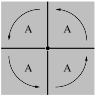
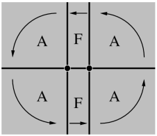
The CTM equations can best be understood by their graphical interpretation, thinking of the matrices as transfer matrices. This is illustrated in Figure 1. The $A$ matrices are interpreted as the transfer matrix of a quarter of a plane (or corner transfer matrix), given the value of the spin at the corner, whereas the $F$ matrices are interpreted as a ‘half-row’ transfer matrix, given the two spins at the end.

(a) $A(a)$

(b) $F(a,b)$

Figure 1: Graphical interpretation of the matrices in the CTM equations.

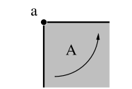
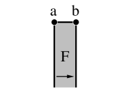
With these interpretations of the matrices, the CTM equations can be intuitively seen to be correct, as shown in Figure 2. Equation 1 corresponds to adding a row onto half a plane, which multiplies the matrix by a constant factor but otherwise leaves it unchanged. Equation 4 has a similar interpretation, but with the values of two spins fixed.

(a) Equation 1

(b) Equation 4

Figure 2: Graphical interpretation of the CTM equations.

Although this graphical interpretation suggests that each matrix be of dimension $2^{p}\times 2^{p}$ for some $p$, this is not actually necessary — the equations hold at any size. Indeed, as we shall see later, the matrices do not all have to be of the same size for the equations to be consistent.

It is easily seen that the CTM equations are invariant under the transformations:

1. $A(a)\rightarrow cA(a)$;

2. $F(a,b)\rightarrow cF(a,b),\xi\rightarrow c^{2}\xi,\eta\rightarrow c^{2}\eta$; and

3. $A(a)\rightarrow P^{T}(a)A(a)P(a),F(a,b)\rightarrow P^{T}(a)F(a,b)P(b)$, where $P(a)$ is an orthogonal matrix of size $n\times n$.

In particular, transformation 3 means that we can take $A(a)$ to be diagonal, with entries ordered from largest to smallest. Furthermore, transformations 1 and 2 imply that we can then take the top left entries of $A(0)$ and $F(0,0)$ to both be 1. Although this is not implied by the CTM equations, we can often take $F(a,b)=F^{T}(b,a)$, due to reflectional symmetry in the model.

2.2 The renormalization group method

The CTMRG method of Nishino and Okunishi ([29]) calculates successive approximations to finite-size solutions of the CTM equations. The principle behind this method is that the finite-size solution maximises $\kappa$ with respect to the matrices. Since $\sum_{a}A^{4}(a)$ is the partition function of the entire plane, we wish to keep the maximum eigenvalues of the infinite-dimensional solution in the $A$ matrices. To do this we expand these matrices, and then diagonalise them. We then apply the diagonalising transformation, but keep only the largest eigenvalues, so that the matrices are shrunk back to their original size.

More specifically, given initial values for the $A$ and $F$ matrices, we expand our $A$ matrices via

$$A_{l}(a)=\left(\begin{array}[]{cc}\sum_{b}\omega\left(\begin{array}[]{cc}a&0\\ 0&b\end{array}\right)F(0,b)A(b)F(b,0)&\sum_{b}\omega\left(\begin{array}[]{cc}a&1\\ 0&b\end{array}\right)F(0,b)A(b)F(b,1)\\ \sum_{b}\omega\left(\begin{array}[]{cc}a&0\\ 1&b\end{array}\right)F(1,b)A(b)F(b,0)&\sum_{b}\omega\left(\begin{array}[]{cc}a&1\\ 1&b\end{array}\right)F(1,b)A(b)F(b,1)\end{array}\right).$$ (5)

We expand the $F$ matrices in a similar fashion:

$$F_{l}(a,b)=\left(\begin{array}[]{cc}\omega\left(\begin{array}[]{cc}a&b\\ 0&0\end{array}\right)F(0,0)&\omega\left(\begin{array}[]{cc}a&b\\ 0&1\end{array}\right)F(0,1)\\ \omega\left(\begin{array}[]{cc}a&b\\ 1&0\end{array}\right)F(1,0)&\omega\left(\begin{array}[]{cc}a&b\\ 1&1\end{array}\right)F(1,1)\end{array}\right).$$ (6)

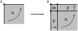
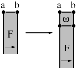
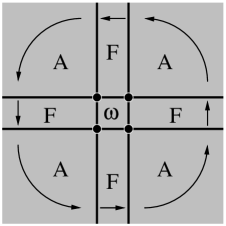
As before, these equations have graphical interpretations, shown in Figure 3. We expand $A(a)$ by adding the weight of two half-rows and a single cell. This has the result of doubling the size of $A(a)$. We add the weight of a single cell to $F(a,b)$, which also doubles its size.

(a) Expanding $A(a)$

(b) Expanding $F(a,b)$

Figure 3: Graphical interpretation of matrix expansion in the CTMRG method.

Next we must reduce both these matrices. This is done by diagonalising $A_{l}(a)$, and then truncating the diagonalising matrix so that only the $n$ largest eigenvalues are kept. To reduce the size of the $F$ matrices, we apply a transformation consistent with transformation 3 in the previous section. If we wish to change the finite size of the solution, we can simply keep a larger number of eigenvalues of $A_{l}(a)$.

The CTMRG method can now be stated in full:

1. Start with initial approximations for $A(a)$ and $F(a,b)$.

2. Calculate $A_{l}(a)$ and $F_{l}(a,b)$ from Equations 5 and 6.

3. Diagonalize $A_{l}(a)$, i.e. find orthogonal matrices $P_{l}(a)$ such that $P_{l}^{T}(a)A_{l}(a)P_{l}(a)$ is diagonal, with diagonal entries in order from largest to smallest.

4. If we want to expand the matrices, increase $n$.

5. Let $P(a)$ be the first $n$ columns of $P_{l}(a)$.

6. Set $A(a)=P^{T}(a)A_{l}(a)P(a)$ and $F(a,b)=P^{T}(a)F_{l}(a,b)P(b)$.

7. Return to step 2.

Since this method does not explicitly calculate $\xi$ or $\eta$, we calculate the partition function per site $\kappa$ by the formula

$$\kappa=\frac{\left(\mbox{Tr }\sum_{a}A^{4}(a)\right)\left(\mbox{Tr }\sum_{a,b,c,d}\omega\left(\begin{array}[]{cc}a&b\\ c&d\end{array}\right)A(a)F(a,c)A(c)F(c,d)A(d)F(d,b)A(b)F(b,a)\right)}{\left(\mbox{Tr }\sum_{a,b}A^{2}(a)F(a,b)A^{2}(b)F(b,a)\right)^{2}}.$$ (7)

In practice, we actually use $A_{l}$ and $F_{l}$ in place of $A$ and $F$ in the above formula.

This formula also has a graphical interpretation, shown in Figure 4. All terms are partition functions of the entire plane, but the term in the denominator contains one column more than the first term in the numerator, while the second term in the numerator contains both a row and a column more than the first term. The net effect is to isolate the partition function of a single cell.

(a) First term in the numerator

(b) Term in the denominator

(c) Second term in the numerator

Figure 4: Terms in Equation 7.

It is also easy to calculate the magnetisation via the formula

$$M=\frac{\mbox{Tr }\sum_{a}aA^{4}(a)}{\mbox{Tr }\sum_{a}A^{4}(a)}.$$

3 Implementing CTMRG for series

Although the CTMRG method has so far been only used for numerical calculations, it can work as a series-calculating tool. In this section, we discuss some difficulties that are specific to series calculations. We also mention some improvements which we have made.

3.1 Modular arithmetic

A standard ‘trick’ in series calculations of long length is to perform all the calculations in integers modulo a prime. If the series that we are calculating has integer coefficients, and we know the sign of each coefficient (which is the case for the hard squares model), then we can repeat the calculations using different moduli and use the Chinese Remainder Theorem to reconstruct the original coefficients.

This difficulty of doing this in this particular algorithm arises because we need to take the square roots of some numbers (for example when normalising eigenvectors). This is partially overcome by the following lemma (taken from [25, Section II.2]).

Lemma 3.1.

Let $p$ be a prime number such that $p\equiv 3\mbox{ mod }4$, and let $a$ be an integer. Then if $a$ has a square root modulo $p$, $a^{\frac{p+1}{4}}$ is a square root of $a$ modulo $p$.

This lemma is easily proved — one such proof is in [12]. Unfortunately, this still does not fully solve the problem, as not all integers have square roots modulo $p$ — this can be seen by noting that each number which has a square root has 2 distinct square roots. At small matrix sizes, this did not seem to be a problem, but at larger sizes, some of the eigenvalues of $A_{l}(a)$ contained square roots which were not calculable. In order to address this, we use block eigenvalues, which we describe below in Section 3.4.

3.2 Unequal matrix sizes

In the CTM equations and the renormalization group method, all the $A$ and $F$ matrices are always of the same size as each other. However, this is not necessary, as the equations can be made consistent with different size matrices. Table 1 shows the sizes needed.

Matrix	Size (equal sizes)	Size (unequal sizes)
$A(0),F(0,0)$	$n\times n$	$n_{1}\times n_{1}$
$A(1)$	$n\times n$	$n_{2}\times n_{2}$
$F(0,1)$	$n\times n$	$n_{1}\times n_{2}$
$F(1,1)$	$n\times n$	$n_{2}\times n_{2}$
$A_{l}(0),A_{l}(1),F_{l}(0,0),F_{l}(0,1)$	$2n\times 2n$	$(n_{1}+n_{2})\times(n_{1}+n_{2})$
$P(0)$	$2n\times n$	$(n_{1}+n_{2})\times n_{1}$
$P(1)$	$2n\times n$	$(n_{1}+n_{2})\times n_{2}$

Table 1: Required sizes for the matrices.

The ability to set the matrices to different sizes is useful because the number of correct series terms derived at each finite size depends on the largest eigenvalue of $A_{l}(a)$ that is missing from $A(a)$ (this will be discussed further in Section 4). However, the leading powers of the eigenvalues of $A_{l}(1)$ increase more rapidly than those of $A_{l}(0)$, so we can keep $A_{l}(1)$ at a smaller size and still derive the same number of terms.

3.3 Diagonalization of a matrix of series

In step 3 of the CTMRG method, we diagonalize a matrix which has power series elements. Furthermore, in order to obtain series exactly to some order, the diagonalization must be exact to that order. In theory, this is impossible even for real-valued matrices. However, $A_{l}(a)$ often turns out to have a relatively simple structure which enables us to diagonalize it exactly.

We first used the well-known power method to calculate the eigenvalues and eigenvectors of $A_{l}(a)$. The following theorem justifies its use in this case. In this theorem and all other cases, we order series in lexicographical order, so that a series with a lower leading power is always considered larger than one with a higher leading power.

Theorem 3.2.

Let $A$ be a symmetric $n\times n$ matrix of power series, with eigenvalues $\lambda_{1}\geq\lambda_{2}\geq\ldots\geq\lambda_{n}$ with leading powers $l_{1},\ldots,l_{n}$ and corresponding eigenvectors $\mathbf{x}_{1},\ldots,\mathbf{x}_{n}$, which are taken to have unit norm. Suppose that we have an estimate $\hat{\mathbf{x}}_{1}$ of $\mathbf{x}_{1}$ which is also of unit norm and accurate to $m$ terms, i.e.

$$\hat{\mathbf{x}}_{1}-\mathbf{x}_{1}=O(z^{m}).$$

Then

$$\|A\hat{\mathbf{x}}_{1}\|-\lambda_{1}=O(z^{l_{1}+m})$$

and

$$\frac{A\hat{\mathbf{x}}_{1}}{\|A\hat{\mathbf{x}}_{1}\|}-\mathbf{x}_{1}=O(z^{m+l_{2}-l_{1}}).$$

Proof.

Write

$$\hat{\mathbf{x}}_{1}-\mathbf{x}_{1}=a_{1}\mathbf{x}_{1}+a_{2}\mathbf{x}_{2}+\ldots+a_{n}\mathbf{x}_{n}$$

where $a_{i}=O(z^{m})$ for all $i$. Then

$$A\hat{\mathbf{x}}_{1} = (1+a_{1})A\mathbf{x}_{1}+a_{2}A\mathbf{x}_{2}+\ldots+a_{n}A\mathbf{x}_{n}$$

$$= (1+a_{1})\lambda_{1}\mathbf{x}_{1}+a_{2}\lambda_{2}\mathbf{x}_{2}+\ldots+a_{n}\lambda_{n}\mathbf{x}_{n}$$

$$= (1+a_{1})\lambda_{1}\mathbf{x}_{1}+O(z^{l_{2}+m})$$

$$\|A\hat{\mathbf{x}}_{1}\| = (1+a_{1})\lambda_{1}+O(z^{l_{2}+m})$$

$$= \lambda_{1}+O(z^{l_{1}+m}).$$

Normalising (with some abuse of $O$-notation) gives

$$\frac{A\hat{\mathbf{x}}_{1}}{\|A\hat{\mathbf{x}}_{1}\|} = (1+O(z^{l_{2}+m-l_{1}}))^{-1}\mathbf{x}_{1}+\frac{O(z^{l_{2}+m})}{O(z^{l_{1}})}$$

$$= \mathbf{x}_{1}+O(z^{m+l_{2}-l_{1}}).$$

∎

Theorem 3.2 shows that if the maximum eigenvalue of $A_{l}(a)$ is not degenerate to leading power, then every iteration of the power method produces more correct terms than the previous iteration, in both the eigenvalue and the eigenvector. If this occurs, we find the dominant eigenvalue using the power method, then deflate the matrix by normalising the eigenvector and calculating

$$A_{l}(a)-\lambda\mathbf{x}\mathbf{x}^{T}.$$

This matrix has the same eigenvalues and eigenvectors of $A_{l}(a)$, but with $\lambda$ replaced by 0.

While the converse of Theorem 3.2 — if the maximum eigenvalue of the matrix is degenerate to leading power, then the power method fails — is not always true, it sometimes holds. In these cases, we cannot use the power method. To overcome this, we shift the eigenvalues and invert. $(A-\lambda_{0}I)^{-1}$ has the same eigenvectors as $A$, but any eigenvalue $\lambda$ becomes $\frac{1}{\lambda-\lambda_{0}}$. We use this if we know the leading terms of one of the eigenvalues of $A_{l}(a)$ to an order which specifies it uniquely. If we know that $\lambda_{0}$ is equal to exactly one of the eigenvalues of $A_{l}(a)$ up to order $z^{m}$, then $A_{l}(a)-\lambda_{0}I$ will have one eigenvalue with leading power $z^{m}$, with all other eigenvalues having smaller leading power. Hence $(A_{l}(a)-\lambda_{0}I)^{-1}$ will have a largest eigenvalue which is not degenerate to leading power, and we can use the power method on this matrix.

In fact, because the convergence of the power method depends on the difference in leading powers between the two largest eigenvalues, if we have a very good approximation of the required eigenvalue, shifting and inverting will result in a matrix which enables us to converge to the correct eigenvalue very quickly.

This leaves us with the problem of finding the first few terms of all the eigenvalues of $A_{l}(a)$ with enough precision to uniquely identify them. In practice, at small size almost all of the eigenvalues of $A_{l}(a)$ have distinct leading terms, if not necessarily leading powers (the first case of identical leading terms occurs at size 23 in $A_{l}(0)$), so it is usually sufficient to find the first term of each eigenvalue. We used various methods:

• The eigenvalues do not change much from iteration to iteration (of the CTMRG method). We use eigenvalues from the previous iteration as starting points, and can converge to the new eigenvalues in very few power method iterations. However, when we expand the matrices, we have one eigenvalue too few, so this is not always sufficient.

• Sometimes, applying a few iterations of the power method does produce the leading term of the largest eigenvalue, even if that eigenvalue is degenerate to leading power. It is usually obvious when this happens, because the leading term becomes invariant within 2-3 iterations.

• If the lowest leading power in $A_{l}(a)$ is $z^{m}$, then $[z^{m}]A_{l}(a)$ has eigenvalues which are the coefficients of $z^{m}$ in the eigenvalues of $A_{l}(a)$. Often, there will only be a few components of $A_{l}(a)$ with leading power $z^{m}$, and these will often break down into a simple block diagonal structure. If one of the blocks is of size $1\times 1$, then that contains the leading term for an eigenvalue.

• If one of the blocks is of size $2\times 2$, then we can calculate leading terms for two eigenvalues by manually solving the eigenvalue equation for that $2\times 2$ block.

• If all else fails, we use block eigenvalues. This is described in the following section.

3.4 Block eigenvalues

In the diagonalization step of the CTMRG method, it is not really important to exactly diagonalize $A_{l}(a)$. All we need to do is to apply a similarity transformation to $A_{l}(a)$ which reduces it to the required size while keeping the largest eigenvalues. Certainly, diagonalizing is one way to ensure that this happens, but it is not the only way. The idea behind block eigenvalues is that they keep the required eigenvalues, while (potentially) avoiding calculational pitfalls which may occur if we diagonalize fully. Formally:

Definition 3.3.

Let $A$ be a symmetric $n\times n$ matrix. A $2\times 2$ matrix $L$ is a block 2-eigenvalue of $A$ with corresponding block 2-eigenvector $Y$, where $Y$ is an $n\times 2$ matrix, if

$$AY=YL.$$

Block $k$-eigenvalues (where $k>2$) are defined in an identical manner, and all results from this section can be extended to larger $k$. The next theorem shows that block 2-eigenvalues have the property of only ‘representing’ 2 eigenvalues.

Theorem 3.4.

Let $A$ be a symmetric $n\times n$ matrix with no degenerate eigenvalues, and let $L$ be a block 2-eigenvalue of $A$ with corresponding block 2-eigenvector $Y$. Then the columns of $Y$ are linear combinations of at most two eigenvectors $\mathbf{x}_{1}$ and $\mathbf{x}_{2}$ of $A$. Furthermore, if the columns of $Y$ are linear combinations of two eigenvectors, then $L$ has eigenvalues $\lambda_{1}$ and $\lambda_{2}$, which are the eigenvalues of $A$ corresponding to $\mathbf{x}_{1}$ and $\mathbf{x}_{2}$.

Proof.

Suppose that the columns of $Y$ are linear combinations of 3 eigenvectors of $A$:

$$Y=\left[\begin{array}[]{c|c}a_{1}\mathbf{x}_{1}+a_{2}\mathbf{x}_{2}+a_{3}\mathbf{x}_{3}&b_{1}\mathbf{x}_{1}+b_{2}\mathbf{x}_{2}+b_{3}\mathbf{x}_{3}\end{array}\right].$$

Let

$$L=\left[\begin{array}[]{cc}l_{11}&l_{12}\\ l_{21}&l_{22}\end{array}\right].$$

Then

$$AY = \left[\begin{array}[]{c|c}a_{1}A\mathbf{x}_{1}+a_{2}A\mathbf{x}_{2}+a_{3}A\mathbf{x}_{3}&b_{1}A\mathbf{x}_{1}+b_{2}A\mathbf{x}_{2}+b_{3}A\mathbf{x}_{3}\end{array}\right]$$

$$= \left[\begin{array}[]{c|c}a_{1}\lambda_{1}\mathbf{x}_{1}+a_{2}\lambda_{2}\mathbf{x}_{2}+a_{3}\lambda_{3}\mathbf{x}_{3}&b_{1}\lambda_{1}\mathbf{x}_{1}+b_{2}\lambda_{2}\mathbf{x}_{2}+b_{3}\lambda_{3}\mathbf{x}_{3}\end{array}\right]$$

$$= YL$$

$$= \big{[}\;\;l_{11}\left(a_{1}\mathbf{x}_{1}+a_{2}\mathbf{x}_{2}+a_{3}\mathbf{x}_{3}\right)+l_{21}\left(b_{1}\mathbf{x}_{1}+b_{2}\mathbf{x}_{2}+b_{3}\mathbf{x}_{3}\right)$$

$$\hskip 28.45274pt\big{|}\;\;l_{12}\left(a_{1}\mathbf{x}_{1}+a_{2}\mathbf{x}_{2}+a_{3}\mathbf{x}_{3}\right)+l_{22}\left(b_{1}\mathbf{x}_{1}+b_{2}\mathbf{x}_{2}+b_{3}\mathbf{x}_{3}\right)\;\;\big{]}$$

$$= \big{[}\;\;(a_{1}l_{11}+b_{1}l_{21})\mathbf{x}_{1}+(a_{2}l_{11}+b_{2}l_{21})\mathbf{x}_{2}+(a_{3}l_{11}+b_{3}l_{21})\mathbf{x}_{3}$$

$$\hskip 28.45274pt\big{|}\;\;(a_{1}l_{12}+b_{1}l_{22})\mathbf{x}_{1}+(a_{2}l_{12}+b_{2}l_{22})\mathbf{x}_{2}+(a_{3}l_{12}+b_{3}l_{22})\mathbf{x}_{3}\;\;\big{]}.$$

This implies that

$$a_{1}l_{11}+b_{1}l_{21} = a_{1}\lambda_{1}$$

$$a_{1}l_{12}+b_{1}l_{22} = b_{1}\lambda_{1}$$

and hence that $\left[\begin{array}[]{cc}a_{1}&b_{1}\end{array}\right]$ is a left eigenvector of $L$ with corresponding eigenvalue $\lambda_{1}$. Similarly, $\left[\begin{array}[]{cc}a_{2}&b_{2}\end{array}\right]$ and $\left[\begin{array}[]{cc}a_{3}&b_{3}\end{array}\right]$ are also left eigenvectors of $L$ with corresponding eigenvalues $\lambda_{2}$ and $\lambda_{3}$ respectively. But $L$ is a $2\times 2$ matrix, and so can have at most 2 distinct eigenvalues, and from our assumptions, $\lambda_{1},\lambda_{2},$ and $\lambda_{3}$ are distinct. This is a contradiction, so the columns of $Y$ can be spanned by at most 2 eigenvectors of $A$. The second part of the theorem now follows from the observed eigenvalues of $L$.

∎

It is easy to see that the converse of this theorem is also true: any two linear combinations of two eigenvectors form a block 2-eigenvector.

We observe that block eigenvalues are not unique, even if we fix the eigenvalues of $A$ which they contain. For example, if $A$ is itself $2\times 2$ with eigenvalues $\lambda_{1}$ and $\lambda_{2}$, then both $\mbox{diag}(\lambda_{1},\lambda_{2})$ and $A$ itself are block 2-eigenvalues of $A$. It is this flexibility that allows us to select block eigenvalues which are easy to compute.

We modify the power method to find block eigenvalues. This method is as follows:

1. Choose two indices $i$ and $j$.

2. Start with an estimate of the block 2-eigenvector $Y_{0}$, with $(Y_{0})_{\{i,j\}}=I_{2}$, where $(Y_{0})_{\{i,j\}}$ is the submatrix of $Y_{0}$ formed by taking rows $i$ and $j$. Set $k=0$.

3. Calculate $AY_{k}$.

4. Set $L_{k}=(Y_{0})_{\{i,j\}}$.

5. Set $Y_{k+1}=AY_{k}L_{k}^{-1}$.

6. Set $k=k+1$.

7. If $k$ does not exceed some fixed value, return to step 3.

8. Apply Gram-Schmidt orthogonalization to the columns of $Y_{k}$.

9. Set $L_{k}=Y^{T}_{k}AY_{k}$.

10. $L_{k}$ and $Y_{k}$ are the estimates for the block 2-eigenvalue and block 2-eigenvector respectively.

In step 1, $i$ and $j$ are chosen to coincide with a $2\times 2$ block of the leading power of $A_{l}(a)$. Steps 8 and 9 ensure that the columns of the approximate block eigenvector are orthonormal.

The following theorem justifies this method. Its proof is an extended version of Theorem 3.2 and will not be shown.

Theorem 3.5.

Let $A$ be a matrix of power series satisfying the conditions of Theorem 3.2. Let $Y=\left[\begin{array}[]{c|c}\mathbf{y}_{1}&\mathbf{y}_{2}\end{array}\right]$, where $\mathbf{y}_{1}$ and $\mathbf{y}_{2}$ are linear combinations of $\mathbf{x}_{1}$ and $\mathbf{x}_{2}$ such that $\mathbf{y}_{1},\mathbf{y}_{2}=O(1)$ and for some indices $i$ and $j$, $Y_{\{i,j\}}=I_{2}$. Then $Y$ is a block 2-eigenvector of $A$ with block 2-eigenvalue $L$, say. Suppose we have an estimate $\hat{Y}$ of $Y$ which also has $\hat{Y}_{\{i,j\}}=I_{2}$ and is accurate to $m$ terms, i.e.

$$\hat{Y}-Y=O(z^{m}).$$

Then

$$\hat{L}=(A\hat{Y})_{\{i,j\}}=L+O(z^{l_{1}+m})$$

and

$$A\hat{Y}\hat{L}^{-1}=Y+O(z^{m+l_{3}-l_{2}}).$$

This theorem shows that if the 2nd and 3rd largest eigenvalues of $A_{l}(a)$ are non-degenerate to leading power, using the modified power method with block 2-eigenvalues gives us a block 2-eigenvalue and associated 2-eigenvector. Therefore, if the first non-degeneracy occurs between the $k$th and ($k+1$)th largest eigenvalues, we will use block $k$-eigenvalues.

Once we have found the block eigenvalues, we must also deflate the matrix. The following theorem gives us the relevant formula.

Theorem 3.6.

Let $A$ be a symmetric matrix with block 2-eigenvalue $L$ and corresponding 2-eigenvector $Y$. Suppose that $Y^{T}Y=I$, and that $L$ has eigenvalues $\lambda_{1}$ and $\lambda_{2}$ (which are also eigenvalues of $A$). Then

$$A-YLY^{T}$$

has the same eigenvectors as $A$, and with the same corresponding eigenvalues, except that $\lambda_{1}$ and $\lambda_{2}$ are replaced by 0.

Proof.

From Theorem 3.4, we know that the columns of $Y$ are spanned by two eigenvectors of $A$, say $\mathbf{x}_{1}$ and $\mathbf{x}_{2}$. Let $\mathbf{x}$ be a different eigenvector of $A$ with corresponding eigenvalue $\lambda$. Then

$$(A-YLY^{T})\mathbf{x}=A\mathbf{x}-YLY^{T}\mathbf{x}=\lambda\mathbf{x}$$

so $\lambda$ is an eigenvalue of the deflated matrix. On the other hand,

$$(A-YLY^{T})Y=AY-YLI=0$$

so any eigenvalue associated with $Y$ is set to 0.

∎

3.5 Model-specific adjustments

Most of the adjustments we made to the method are applicable to any model. However, we did make some adjustments which are specific to the hard squares model. The most important arises from the fact that by definition, $F(1,1)$ must be the zero matrix. Furthermore, it is easy to see from Equation 5 that only the top left $n_{1}\times n_{1}$ block of $A_{l}(1)$ is nonzero. This enables us to treat $A_{l}(1)$ as a $n_{1}\times n_{1}$ matrix, which makes manipulation faster. We note that in the case where the sizes are equal ($n_{1}=n_{2}$), this means that we are calculating and keeping all of the eigenvalues of $A_{l}(1)$.

This latter point did in fact trip us up somewhat: when we tried to calculate and keep an extra eigenvalue (which should be 0), we produced a series with very high leading power, and gibberish for the eigenvector. Naturally this led to chaos when we tried to reduce the other matrices and repeat!

4 Convergence

If we use Equation 7 as written to calculate $\kappa$, the number of series terms we obtain is given by the largest eigenvalue of the $A_{l}$ matrices that we leave out in the shrinking step. More precisely, if the largest missing eigenvalue has leading power $z^{a}$, then the first term that is wrong in the approximation of $\kappa$ is $z^{4a}$. This is because all terms in Equation 7 involve 4th powers of the $A$ matrices. Table 2 shows the number of terms that we would produce if one matrix was limited in size and the other was unlimited.

Size of $A(0)$	Number of terms	Size of $A(1)$	Number of terms
1	8	1	17
2	16	2	25
3	24	3	33
4-5	32	4	41
6-7	40	5	45
8-10	48	6	49
11-13	56	7-8	57
14-17	64	9-11	65
18	68	12-14	73
19-22	72	15-18	81
23-28	80	19	85
29	88	20	89

Table 2: Number of correct series terms from each matrix.

However, as we remarked after Equation 7, in practice we use $A_{l}$ and $F_{l}$ in place of $A$ and $F$ in this equation to calculate $\kappa$. It is now much less obvious how many terms we now derive. We calculated the number of correct terms at each size by comparing series resulting from small sizes with known terms from larger sizes. The results are in Table 3.

		Number of terms	Number of terms
Size of $A(0)$	Size of $A(1)$	from small matrices	from large matrices
2	2	16	20
3	3	24	28
4	4	32	36
5	5	32	38
6	6	40	44
7	7	40	46
8	8	48	52
9	9	48	52
10	10	48	54
11	11	56	60
12	12	56	60
13	13	56	62
14	14	64	68
15	15	64	68
16-17	15	64	70
18	15	68	76
19-21	15	72	76
22	15	72	78

Table 3: Number of correct series terms using small and large matrices.

It is apparent that if we set a desired number of terms, then set the matrices to the smallest size able to derive this number of terms, then using large matrices gives us 4 extra terms. Furthermore, if we use the largest size possible, using large matrices gives us 6 extra terms if this size is different. The only exception to this rule occurs at size $(n_{1},n_{2})=(18,15)$, which can be considered a special case in the sense that every other size produces a number of terms which is a multiple of 8.

Using this information, we ran the CTMRG method for sizes up to $(n_{1},n_{2})=(29,20)$, and were able to determine that this yields 92 terms for the partition function per site.

One question of interest is whether the method is indeed an $O(\alpha^{\sqrt{n}})$ method, where $n$ is now the number of terms derived. For this to be true, we would need the matrix size (which we denote by $m$ for this argument) to also grow like $O(\beta^{\sqrt{n}})$. Empirical evidence does indeed suggest that this relationship holds. Figure 5 shows a plot of the logarithm of the matrix size against the square root of the number of terms, and it can be seen that a linear relationship is quite strongly apparent.

Figure 5: Matrix size vs. number of terms.

The line fits have very close to the same slope, and it seems reasonable to conjecture that the true slopes are indeed identical. Taking the maximum of the two fitted slopes gives us $\beta\approx 1.69$. Now the CTMRG method is theoretically an $O(m^{3})$ method if the shifted inverse power method is not used, and $O(m^{4})$ otherwise, although in practice the latter case is more efficient. This gives us an estimate of $\alpha\approx 4.85$ for the former case and $\alpha\approx 8.21$ for the latter.

5 Analysis

It must be noted that the focus of this paper is on the CTMRG method used to generate the hard squares series, rather than results obtained from analysing the resulting series. Nevertheless, the series is much longer than anything previously generated, so we analyse it to see what results can be obtained.

The series which we have generated is the low-density series, where all spins are 0 in the base state. This series was generated to 43 terms by Baxter et al. in [10], but was not used for analysis, as they preferred the high-density series (the expansion in the variable $z^{-1}$), which was also generated via CTM. Unfortunately, we have so far been unable to generate this series with CTMRG.

Two points of interest in the hard squares model are the critical point at $z_{c}\approx 3.80$, and the dominant singularity at $z\approx-0.12$. The critical point is of interest because it is the transition point where one sublattice becomes preferentially occupied, i.e. the model changes from low- to high-density. However, because the dominant singularity for the low-density series is much closer to 0, this tends to ‘drown out’ information about the critical point, so it is easier to analyse the high-density series for information about this point. Indeed, to our knowledge the low-density series has not been used to analyse the critical point since 1965 ([19]).

Our series is of sufficient length that we can make a reasonably accurate determination of the critical point. To do this, we analysed the magnetisation series

$$M(z)=\frac{d}{dz}\ln\kappa$$

using the method of differential approximants ([21]). In short, this method fits a function to the series which satisfies a low-order differential equation with polynomial coefficients, then looks at the singularity structure of the fitted function. The critical exponent of the magnetisation series is $1-\alpha$, where $\alpha$ is the specific heat exponent. Using homogeneous second-order approximants, we found

$$z_{c}=3.79635(9),\alpha=0.0020(17),$$

where the numbers in brackets are twice the standard deviation of the approximant estimates (though we note that this should not be taken as strict error bounds). These numbers are in line with the commonly held view that this model belongs to the Ising universality class, where $\alpha=0$. They are also consistent with, though considerably less accurate than, the best estimates attained by high-density analysis (see for example [24]).

A much more accurate determination can be made of the dominant unphysical singularity, also using differential approximants. This point is primarily of interest because it is known ([15]) that $M(-z)$ is the generating function of directed animals on the body-centred cubic (b.c.c.) lattice. Again using second-order approximants, we derived (where $\gamma$ is the negative exponent of the singularity)

$$z=0.1193388818(6),\gamma=0.171(14).$$

In addition, we can then use these estimates to estimate the critical amplitude by solving for various $n$ the equation

$$c_{n}=A(1/z)^{n}n^{\gamma-1}$$

and then plotting our results against $1/n$. This gives

$$A=0.145,$$

though we would hesitate to give an error for this estimate. This results in a formula for the asymptotic growth of the number of directed b.c.c. animals as

$$c_{n}\sim 0.145\times 8.379^{n}n^{-0.829}.$$

6 Conclusion

In this paper, we have given a large amount of detail as to how to adapt the CTMRG method to derive series expansions, illustrating by calculating 92 terms of the hard squares partition function per site. A number of technical difficulties have been overcome, notably with the use of block eigenvalues.

It is clear that the method is very efficient for calculating series, and we are fairly confident in saying that it appears to be an $O(\alpha^{\sqrt{n}})$ method, at least for hard squares. If this is true, theoretically this represents a vast improvement over all other non-CTM based methods, which are exponential-time.

The CTMRG is by nature a very general method, theoretically applicable to any IRF model. Although in practice certain symmetry requirements are also necessary, we are certain that its scope is not limited to the hard squares model, and believe that it can be successfully applied to many models to derive series.

In particular, although the original formulation of the CTMRG is for spin models, we are currently engaged in adapting it to vertex and bond models, where the ‘spin’ values lie on the bonds of the lattice. If this is successful, this would open up a whole new category of models which we can apply this method to.

Appendix A The hard squares partition function

$n$	Coefficient of $z^{n}$
0	1
1	1
2	-2
3	8
4	-40
5	225
6	-1362
7	8670
8	-57253
9	388802
10	-2699202
11	19076006
12	-136815282
13	993465248
14	-7290310954
15	53986385102
16	-402957351939
17	3028690564108
18	-22904845414630
19	174175863324830
20	-1331044586131594
21	10217222223168657
22	-78746146809812974
23	609153211886323748
24	-4728123941310119629
25	36812657530897835053
26	-287439461791025474818
27	2250314840062625743472
28	-17660572072127314002800
29	138917347311377551474338
30	-1095044102004611782219794
31	8649079543673381406386578
32	-68441069128808194161922385
33	542528768962390004584576547
34	-4307673277782673209498570830
35	34255913017196256622645849406
36	-272811973711116137449858922289
37	2175663718003877171512666515965
38	-17373555504340949646557187291612
39	138907228460715779361866368091340
40	-1111918671840441187102586337375728
41	8910623138600432871714003453719826
42	-71483639721296620300995136065253668
43	574046483511726716038779843196291148
44	-4614334493396507062886044646610429157
45	37125630601616372118866371971750653400
46	-298967336036118129407418784080218615722
47	2409585254960886275025134297727824908884
48	-19436320799533420112481773783042415629261
49	156900573920162022290578129250670083086420
50	-1267535404869110564352411619174739265523868
51	10247264495520354226129600890924108669994610
52	-82900281399057902108151873229350373092209619
53	671108737638240713935447505566478276195162695
54	-5436355713698184882980887629568939260561976810
55	44064694805175046617091994106334371203302938776
56	-357381432990462157109211753457839726558288436818
57	2900163105083745845730874102786889605714746995342
58	-23547968769944310985596027746076562077618218334718
59	191300842560899308725071542860775532916665485120184
60	-1554908876921181737147789458998481638358161928897591
61	12644749797865196843555951541679953304124755960793511
62	-102878765260913100430709623218183178373090721871184044
63	837422752069874189432173744615001497684269956054808622
64	-6819631352357213787230910331148600271798284788605855567
65	55560748326532902393539847760004905789472334071550252840

$n$	Coefficient of $z^{n}$
66	-452856402854393303217557453525610814293298860266644333788
67	3692603110457838500058306311991565464177314769422347258712
68	-30121676657343800172725754276632905777873884902459021355361
69	245807413474990027756549514844805809793849952994063754626736
70	-2006666888019302099239255549634083582058527531632344348155382
71	16387602447917907925939835398242666596145404236646122967314476
72	-133878529017269645222962908444675311373581968623046805553003420
73	1094101349658594729612361555133529988788157463539921142705674406
74	-8944399559315399008297389300844640091529020258243919220987964946
75	73145551008354781012338946915052673817209937064486329418176787110
76	-598361927886673095890838492285516107595411125515110286142445348366
77	4896386322427075789832417441388661081060656557690205676073687691148
78	-40079251232688073115885503442096697172216907602724038749014964900102
79	328165082254688810946984293011935816745304828942186642808616061608366
80	-2687761676918736119845722240766742417562922822567399217372718456286685
81	22019713136269272910821806308408983339580368950205667984685424553851833
82	-180448000438033885658918793091063759646692376290415150089214756908058884
83	1479139461040169224120227477170760620707156578769244001285571905105338718
84	-12127744073180764329413943869671758523793164836282542085455077710510119460
85	99463122933872289081188517872014743137876065832109978317420162733094536685
86	-815929689380612324987741425248826191973143825540604664462510726155651011716
87	6694982697997270547775373671241966492741914685730214539163542377702398519634
88	-54947741307877958845071184518809752964246445865955568127226073015990501845122
89	451077911529567493786366696817726882849261112979605658136036057774968937144332
90	-3703841147518398777454506425673146945950304284333846865189410967618798579127030
91	30419357562872572130630138383935901849475451065777199789899946292436298406543592

References

- [1] R. J. Baxter. Corner transfer matrices of the eight-vertex model. I. Low-temperature expansions and conjectured properties. J. Stat. Phys., 15(6):485–503, 1976.
- [2] R. J. Baxter. Corner transfer matrices of the eight-vertex model. II. The Ising model case. J. Stat. Phys., 17(1):1–14, 1977.
- [3] R. J. Baxter. Variational approximations for square lattice models in statistical mechanics. J. Stat. Phys., 19(5):461–478, 1978.
- [4] R. J. Baxter. Hard hexagons: exact solution. J. Phys. A: Math. Gen., 13:L61–L70, 1980.
- [5] R. J. Baxter. Corner transfer matrices of the chiral Potts model. J. Stat. Phys., 63(3-4):433–53, 1991.
- [6] R. J. Baxter. Chiral Potts model: corner transfer matrices and parametrizations. Int. J. Mod. Phys. B, 7(20-21):3489–3500, 1993.
- [7] R. J. Baxter. Corner transfer matrices of the chiral Potts model. II. The triangular lattice. J. Stat. Phys., 70(3-4):535–582, 1993.
- [8] R. J. Baxter. Planar lattice gases with nearest-neighbour exclusion. Ann. Comb., 3(2-4):191–203, 1999.
- [9] R. J. Baxter and I. G. Enting. Series expansions from corner transfer matrices - the square lattice model. J. Stat. Phys., 21(1):103–123, 1979.
- [10] R. J. Baxter, I. G. Enting, and S. K. Tsang. Hard-square lattice gas. J. Stat. Phys., 22(4):465–489, 1980.
- [11] R. J. Baxter and P. J. Forrester. A variational approximation for cubic lattice models in statistical mechanics. J. Phys. A: Math. Gen., 17(13):2675–2685, 1984.
- [12] Y. Chan. Selected problems in lattice statistical mechanics. PhD thesis, The University of Melbourne, 2005.
- [13] T. de Neef. Some applications of series expansions in magnetism. PhD thesis, Eindhoven University of Technology, 1975.
- [14] T. de Neef and I. G. Enting. Series expansions from the finite lattice method. J. Phys. A: Math. Gen., 10(5):801–805, 1977.
- [15] D. Dhar. Equivalence of the two-dimensional directed-site animal problem to baxter’s hard-square lattice-gas model. Phys. Rev. Lett., 49(14):959–982, 1982.
- [16] I. G. Enting and R. J. Baxter. An investigation of the high-field series expansions for the square lattice Ising model. J. Phys. A: Math. Gen., 13(12):3723–3734, 1980.
- [17] D. P. Foster and C. Pinettes. A corner transfer matrix renormalization group investigation of the vertex-interacting self-avoiding walk model. J. Phys. A: Math. Gen., 36:10279–10298, 2003.
- [18] D. P. Foster and C. Pinettes. Corner-transfer-matrix renormalization-group method for two-dimensional self-avoiding walks and other models. Phys. Rev. E, 67(045105), 2003.
- [19] D. S. Gaunt and M. E. Fisher. Hard-sphere lattice gases. I. Plane-square lattice. J. Chem. Phys., 43(8):2840–2863, 1965.
- [20] A. Gendiar and T. Nishino. Latent heat calculation of the three-dimensional and Potts models by the tensor product variational approach. Phys. Rev. E, 65(4):046702, 2002.
- [21] A. J. Guttmann. Asymptotic analysis of power-series expansions. In C. Domb and J. L. Lebowitz, editors, Phase transitions and critical phenomena, volume 13. Academic Press, New York, 1989.
- [22] I. Jensen, A. J. Guttmann, and I. G. Enting. Low-temperature series expansions for the spin-1 Ising model. J. Phys. A: Math. Gen., 27(21):6987–7005, 1994.
- [23] I. Jensen, A. J. Guttmann, and I. G. Enting. Low-temperature series expansions for the square lattice Ising model with spin . J. Phys. A: Math. Gen., 29(14):3805–3815, 1996.
- [24] G. Kamieniarz and H. W. J. Blöte. The non-interacting hard-square lattice gas: Ising universality. J. Phys. A: Math. Gen., 26:6679–6689, 1993.
- [25] N. Koblitz. A course in number theory and cryptography. Springer-Verlag, 1987.
- [26] V. V. Mangazeev, M. T. Batchelor, V. V. Bazhanov, and M. Yu. Dudalev. Variational approach to the scaling function of the 2D Ising model in a magnetic field. J. Phys. A.: Math. Theor., 42(4):042005, 2009.
- [27] V. V. Mangazeev, M. Yu. Dudalev, V. V. Bazhanov, and M. T. Batchelor. Scaling and universality in the two-dimensional Ising model with a magnetic field. Phys. Rev. E, 81:060103(R), 2010.
- [28] T. Nishino, Y. Hieida, K. Okunishi, N. Maeshima, Y. Akutsu, and A. Gendiar. Two-dimensional tensor product variational formulation. Progress of Theoretical Physics, 105(3):409–417, 2001.
- [29] T. Nishino and K. Okunishi. Corner transfer matrix renormalization group method. J. Phys. Soc. Jpn., 65(4):891–894, 1996.
- [30] T. Nishino and K. Okunishi. Corner transfer matrix algorithm for classical renormalization group. J. Phys. Soc. Jpn., 66(10):3040–3047, 1997.
- [31] T. Nishino and K. Okunishi. A density matrix algorithm for 3D classical models. J. Phys. Soc. Jpn., 67(9):3066–3072, 1998.
- [32] T. Nishino and K. Okunishi. Numerical latent heat observation of the potts model. J. Phys. Soc. Jpn., 67(4):1492–1493, 1998.
- [33] T. Nishino and K. Okunishi. Kramers-Wannier approximation for the 3D Ising model. Progress of Theoretical Physics, 103(3):541–548, 2000.
- [34] T. Nishino, K. Okunishi, Y. Hieida, N. Maeshima, and Y. Akutsu. Self-consistent tensor product variational approximation for 3D classical models. Nuclear Physics B, 575(3):504–512, 2000.
- [35] T. Nishino, K. Okunishi, and M. Kikuchi. Numerical renormalization group at criticality. Phys. Lett. A, 213(1-2):69–72, 1996.
- [36] K. Okunishi, Y. Hieida, and Y. Akutsu. Universal asymptotic eigenvalue distribution of density matrices and corner transfer matrices in the thermodynamic limit. Phys. Rev. E, 59(6):R6227–R6230, 1999.
- [37] N. Tsutshima and T. Horiguchi. Phase diagrams of spin-3/2 Ising model on a square lattice in terms of corner transfer matrix renormalization group method. J. Phys. Soc. Jpn., 67(5):1574–1582, 1998.