Multigrid methods for two-player zero-sum stochastic games

Marianne Akian    Sylvie Detournay
Abstract

We present a fast numerical algorithm for large scale zero-sum stochastic games with perfect information, which combines policy iteration and algebraic multigrid methods. This algorithm can be applied either to a true finite state space zero-sum two player game or to the discretization of an Isaacs equation. We present numerical tests on discretizations of Isaacs equations or variational inequalities. We also present a full multi-level policy iteration, similar to FMG, which allows to improve substantially the computation time for solving some variational inequalities.

1 Introduction

In the present paper, we are interested in solving non-linear finite dimensional equations of the form :

v(x)=maxa𝒜(minb(y𝒳μp(y|x,a,b)v(y)+r(x,a,b)))x𝒳.formulae-sequence𝑣𝑥subscript𝑎𝒜subscript𝑏subscript𝑦𝒳𝜇𝑝conditional𝑦𝑥𝑎𝑏𝑣𝑦𝑟𝑥𝑎𝑏for-all𝑥𝒳v(x)\,=\,{\max_{a\in\mathcal{A}}\,\left(\min_{b\in\mathcal{B}}\,\left(\sum_{y\in\mathcal{X}}\mu\,p(y\,|\,x,a,b)\,v(y)\,+\,r(x,a,b)\right)\right)}\qquad\forall x\in\mathcal{X}. (1)

with unknown the function v:𝒳:𝑣𝒳v:\mathcal{X}\rightarrow\mathds{R}, where 𝒳:={1,,n}assign𝒳1𝑛\mathcal{X}:=\left\{{1,\dots,n}\right\}. Here 𝒜:={1,,m1}assign𝒜1subscript𝑚1\mathcal{A}:=\left\{{1,\dots,m_{1}}\right\}, :={1,,m2}assign1subscript𝑚2\mathcal{B}:=\left\{{1,\dots,m_{2}}\right\} are finite sets; the functions (x,a,b)𝒳×𝒜×r(x,a,b)𝑥𝑎𝑏𝒳𝒜𝑟𝑥𝑎𝑏(x,a,b)\in\mathcal{X}\times\mathcal{A}\times\mathcal{B}\rightarrow r(x,a,b)\in\mathds{R} and (x,a,b,y)𝒳×𝒜××𝒳p(y|x,a,b)+𝑥𝑎𝑏𝑦𝒳𝒜𝒳𝑝conditional𝑦𝑥𝑎𝑏subscript(x,a,b,y)\in\mathcal{X}\times\mathcal{A}\times\mathcal{B}\times\mathcal{X}\rightarrow p(y|x,a,b)\in\mathds{R}_{+} are given such that y𝒳p(y|x,a,b)=1subscript𝑦𝒳𝑝conditional𝑦𝑥𝑎𝑏1\sum_{y\in\mathcal{X}}p(y|x,a,b)=1; and 0<μ<10𝜇10<\mu<1 is a given constant. These equations appear when solving the following particular dynamic games.

An infinitely repeated game, or discrete time dynamic game, or infinite horizon multi-stage game, consists in an infinite sequence of state transitions, where at each step, the transition depends on the actions of the players, and each player receives a reward which depends on the state of the game and the actions of all players at this step. The aim of each player is to maximize his own objective function, for instance his payoff which is the sum of the rewards he received at all steps. The game is stochastic when the state sequence is a random process with a Markov property, then the objective function is the expected payoff. It is a two player zero-sum game when there are two players with opposite rewards, hence player 222 aims to minimize player 111 objective function. When the game does not stop in finite time (almost surely), one often consider a discounted payoff where the reward at each step k𝑘k is discounted by some multiplicative factor μksuperscript𝜇𝑘\mu^{k}, with 0<μ<10𝜇10<\mu<1.

Consider in particular a two player zero-sum discounted stochastic game with finite state space 𝒳𝒳\mathcal{X} and action spaces 𝒜𝒜\mathcal{A} and \mathcal{B} for player 111 and player 222 respectively. Denote by r(x,a,b)𝑟𝑥𝑎𝑏r(x,a,b) the reward of player 111 when (at the current step) the state is x𝒳𝑥𝒳x\in\mathcal{X} and the actions of player 111 and 222 are a𝒜𝑎𝒜a\in\mathcal{A}, b𝑏b\in\mathcal{B} respectively. Denote by p(y|x,a,b)𝑝conditional𝑦𝑥𝑎𝑏p(y|x,a,b) the transition probability from state x𝑥x to state y𝑦y when the actions of player 111 and 222 are a𝒜𝑎𝒜a\in\mathcal{A}, b𝑏b\in\mathcal{B} respectively. Assume that player 111 plays before player 222, and that at each step, player 111 is choosing his action a𝒜𝑎𝒜a\in\mathcal{A} as a function of the current state x𝒳𝑥𝒳x\in\mathcal{X}, and player 222 is choosing his action b𝑏b\in\mathcal{B} as a function of the current state x𝒳𝑥𝒳x\in\mathcal{X} and action a𝒜𝑎𝒜a\in\mathcal{A} of player 111. Assume each player is maximizing his own objective function. Under the previous finiteness conditions on (𝒳𝒳\mathcal{X}, 𝒜𝒜\mathcal{A}, \mathcal{B}), there exists a function v:𝒳:𝑣𝒳v:\mathcal{X}\rightarrow\mathds{R} which associates to each x𝒳𝑥𝒳x\in\mathcal{X} the expected payoff v(x)𝑣𝑥v(x) of player 111 when the initial state of the game is x𝑥x. This function is called the value or the value function of the game. It is the unique solution of Equation (1) [54], called itself the dynamic programming equation or Shapley equation of the game. Solving Equation (1) is important since it also gives the optimal stationary strategies of the game, see section 2 for precise definitions of strategies and details. Discrete time zero-sums stochastic games arise in several domains of applications, such as military operations [43], network flow control [4], pursuit-evasion problems (although often studied in the deterministic case), see [46] for other applications references.

Equations of the form (1) can also be obtained as special discretizations of partial differential equations associated to differential stochastic games, where the state space 𝒳𝒳\mathcal{X} is now a subset of dsuperscript𝑑\mathds{R}^{d} (see section 3 for details). For instance the following non-linear elliptic partial differential equation called Isaacs equation :

maxa𝒜(minb(i,j=1dqij(a,b,x)2v(x)xixj+j=1dgj(a,b,x)v(x)xjλv(x)+r(x,a,b)))=0x𝒳subscript𝑎𝒜subscript𝑏superscriptsubscript𝑖𝑗1𝑑subscript𝑞𝑖𝑗𝑎𝑏𝑥superscript2𝑣𝑥subscript𝑥𝑖subscript𝑥𝑗superscriptsubscript𝑗1𝑑subscript𝑔𝑗𝑎𝑏𝑥𝑣𝑥subscript𝑥𝑗𝜆𝑣𝑥𝑟𝑥𝑎𝑏0for-all𝑥𝒳\max_{a\in\mathcal{A}}\,\left(\min_{b\in\mathcal{B}}\,\left(\sum_{i,j=1}^{d}q_{ij}(a,b,x){\displaystyle\frac{\partial^{2}v(x)}{\partial x_{i}\partial x_{j}}}+\sum_{j=1}^{d}g_{j}(a,b,x){\displaystyle\frac{\partial v(x)}{\partial x_{j}}}-\lambda v(x)+r(x,a,b)\,\right)\right)=0\;\;\forall x\in\mathcal{X} (2)

allows one to solve a differential game in the same way as (1) solves a discrete time dynamic game. Here 𝒜𝒜\mathcal{A}, \mathcal{B} are either finite sets or subsets of some psuperscript𝑝\mathds{R}^{p} spaces, λ0𝜆0\lambda\geq 0 is a scalar, and (x,a,b)𝒳×𝒜×q(x,a,b)=(qij(x,a,b))i,j=1,,d𝑥𝑎𝑏𝒳𝒜𝑞𝑥𝑎𝑏subscriptsubscript𝑞𝑖𝑗𝑥𝑎𝑏formulae-sequence𝑖𝑗1𝑑(x,a,b)\in\mathcal{X}\times\mathcal{A}\times\mathcal{B}\rightarrow q(x,a,b)=(q_{ij}(x,a,b))_{i,j=1,\dots,d} Sd+absentsubscriptsuperscript𝑆𝑑\in S^{+}_{d}, the set of positive definite symmetric d×d𝑑𝑑d\times d matrices, (x,a,b)𝒳×𝒜×g(x,a,b)=(gj(x,a,b))j=1,,d𝑥𝑎𝑏𝒳𝒜𝑔𝑥𝑎𝑏subscriptsubscript𝑔𝑗𝑥𝑎𝑏𝑗1𝑑(x,a,b)\in\mathcal{X}\times\mathcal{A}\times\mathcal{B}\rightarrow g(x,a,b)=(g_{j}(x,a,b))_{j=1,\dots,d} dabsentsuperscript𝑑\in\mathds{R}^{d}, and (x,a,b)𝒳×𝒜×r(x,a,b)𝑥𝑎𝑏𝒳𝒜𝑟𝑥𝑎𝑏(x,a,b)\in\mathcal{X}\times\mathcal{A}\times\mathcal{B}\rightarrow r(x,a,b)\in\mathds{R} are given functions. Such equations may be applied in particular to pursuit-evasion games (see for instance [6]), but they also appear in solving Hsuperscript𝐻H^{\infty} optimal control problems (see for instance [9]), or risk-sensitive optimal control problems [32], in particular for finance applications [25]. The discretization of Equation (2) with a monotone scheme in the sense of [8] yields an equation of the form (1) which can then be interpreted as the dynamic programming equation of a stochastic game with discrete time and finite state space. Suitable possible discretizations schemes are for instance : Markov chain discretizations [39, 40], monotone discretizations [8], full discretizations of semi-Lagrangian type [6], and max-plus finite element method [3] for deterministic games or control problems. Hence, we are interested in solving discretizations of Equation (2) which have the form of Equation (1), in order to find an approximation of the value of the corresponding differential stochastic game.

In the presence of a discount factor μ<1𝜇1\mu<1, the nonlinear equation (1) can be solved by applying the fixed point iterations which are called, in the optimal control and game literature, value iterations or the value iteration algorithm [10]. The iterations of this method are cheap but their convergence slows considerably as the discount factor μ𝜇\mu approaches one. Moreover, when we discretize Equation (2) with a finite difference or finite element method with a discretization step hh, we obtain an equation of the form (1) with a discount factor μ=1O(λh2)𝜇1𝑂𝜆superscript2\mu=1-O(\lambda h^{2}), then when hh is small μ𝜇\mu is close to one and the value iteration method is as slow as the Jacobi or Gauss-Seidel iterations for a discretized linear elliptic equation. Another approach consists in the so called policy iteration algorithm, initially introduced by Howard [38] for one player stochastic games (i.e. stochastic control problems). Later adaptations of this algorithm were proposed for the two player games : by Hoffman and Karp [35] for a special mean-payoff case, by Dernado [23] for approximations of value functions in discounted stochastic games, in Puri thesis [49] for discounted stochastic games, and by Cochet-Terrasson and Gaubert [19] for the general mean-payoff case. In all cases, policy algorithm converges faster than the value iteration algorithm and in practice it ends in few steps (see for instance [24] for numerical examples in the case of deterministic games).

A (feedback) policy (or pure Markovian stationary strategy, see Section 2 below) α:𝒳𝒜:𝛼𝒳𝒜{{\alpha}}:\mathcal{X}\rightarrow\mathcal{A} for the first player is a function which maps any x𝒳𝑥𝒳x\in\mathcal{X} to an action a𝒜𝑎𝒜a\in\mathcal{A}. Then, starting with an initial policy for player 111, the policy iteration algorithm for the two player zero-sum stochastic game consists in applying successively a policy evaluation step followed by a policy improvement step. The policy evaluation step amounts to compute the value of the game for the current policy α𝛼{\alpha}, that is the solution v𝑣v of (1) where instead of taking the maximum of the expression inside the “max”, one evaluates it with a=α(x)𝑎𝛼𝑥a={\alpha}(x). The policy improvement step consists in finding the optimal policy for the current value function v𝑣v, that is the policy optimizing the expression inside the “max” in (1) when the value function is v𝑣v. Computing the above value functions (in the policy evaluation steps) is performed using the policy iteration algorithm for a one-player game. The policy iteration algorithm is explained in more general settings in Section 4. It stops after a finite number of steps when the sets of actions are finite, see [41, 14, 50] for one player games and [49, 19] for two player games. In addition, under regularity assumptions on the maps r𝑟r and p𝑝p, the policy iteration algorithm for a one player game with infinite action spaces is equivalent to Newton’s method, thus can have a super-linear convergence in the neighborhood of the solution, see [51, 15] for superlinear convergence under general regularity assumptions, and [51, 2, 5] for order p>0𝑝0p>0 superlinear convergence under additional regularity and strong convexity assumptions.

Each policy iteration for a one player game (or each iteration in the inner loop of the two player algorithm) requires the solution of a linear system. Indeed, when we fix feedback policies α:𝒳𝒜:𝛼𝒳𝒜{\alpha}:\mathcal{X}\rightarrow\mathcal{A} and β:𝒳:𝛽𝒳{\beta}:\mathcal{X}\rightarrow\mathcal{B} for player 111 and 222 respectively, the system of equations (1) yields a linear system of the form : v=μMv+r𝑣𝜇𝑀𝑣𝑟v=\mu Mv+r where v,r𝒳𝑣𝑟superscript𝒳v,r\in\mathds{R}^{\mathcal{X}} are respectively the value function of the game and the vector of rewards for the fixed policies α𝛼{{\alpha}} and β𝛽{\beta}, 0<μ<10𝜇10<\mu<1 is the discount factor and M𝒳×𝒳𝑀superscript𝒳𝒳M\in\mathds{R}^{\mathcal{X}\times\mathcal{X}} is a Markov matrix whose elements are the transition probabilities Mxy=p(x|y,α(x),β(x))+subscript𝑀𝑥𝑦𝑝conditional𝑥𝑦𝛼𝑥𝛽𝑥subscript{M}_{xy}=p(x|y,{\alpha}(x),{\beta}(x))\in\mathds{R}_{+} for x,y𝒳𝑥𝑦𝒳x,y\in\mathcal{X} (and each rowsum of M𝑀M equals one). When the dynamic programming equation (1) is coming from the discretization of an Isaacs partial differential equation (2), this linear system corresponds to the discretization of a linear elliptic partial differential equation, hence it may be solved in the best case in a time in the number of discretization points by using multigrid methods, that is the cardinality |𝒳|𝒳|\mathcal{X}| of the discretized state space 𝒳𝒳\mathcal{X}, or the size of the matrix M𝑀M. For general stochastic games on a finite state space 𝒳𝒳\mathcal{X}, since M𝑀M is a Markov matrix, the matrix (IμM)𝐼𝜇𝑀(I-\mu M) of the linear system is an invertible M-matrix [13], and one may expect the same complexity when solving them by using an algebraic multigrid method.

In the present paper, we consider the combination of policy iterations with the algebraic multigrid method (AMG) introduced by Brandt, McCormick and Ruge [17, 18], see also Ruge and Stüben [53]. We shall call AMGπ𝜋\pi the resulting algorithm. This algorithm can be applied either to a true finite state space zero-sum two player game or to the discretization of an Isaacs equation, although in the present paper we restrict ourselves to numerical tests for the discretization of stochastic differential games, since the AMG algorithm needs some improvements to be applied to arbitrary non symmetric linear systems arising in game problems. Such an association of multigrid methods with policy iteration has already been used and studied in the case of one player games, that is discounted stochastic control problems (see Hoppe [36, 37] and Akian [1, 2] for Hamilton-Jacobi-Bellman equations or variational inequalities, Ziv and Shimkin [48] for AMG with learning methods). However, it is new in the case of two player games. We have implemented this algorithm (in C) and shall present numerical tests on discretizations of Isaacs or Hamilton-Jacobi-Bellman equations or variational inequalities, while comparing AMGπ𝜋\pi with the combination of policy iterations with direct solvers.

The complexity of two player zero-sum stochastic games is still unsettled, one only knows that it belongs to the complexity class of NP\capcoNP [49]. Indeed, the number of policy iterations is bounded by the number of possible policies, which is exponential in the cardinality of 𝒳𝒳\mathcal{X}. Friedmann has shown [34] that a strategy improvement algorithm requires an exponential number of iterations for a “worst”-case family of games called parity games, this result can be extended to other types of zero-sum stochastic games, in particular to mean-payoff and discounted zero-sum stochastic games, and to undiscounted stochastic control problems (one-player games) as shown by Fearnley [27, 28]. However, as for Newton’s algorithm, convergence can be improved by starting the policy iteration with a good initial guess, close to the solution. With this in mind, we present a full multi-level policy iteration, similar to FMG. It consists in solving the problem at each grid level by performing policy iterations until a convergence criterion is verified, then to interpolate the strategies and value to the next level, in order to initialize the policy iterations of the next level, until the finest level is attained. When at each level policy iterations are combined with the algebraic multigrid method, we shall call FAMGπ𝜋\pi the resulting full multi-level policy iteration algorithm. For one-player discounted games with infinite number of actions and under regularity assumptions, one can show [2, 1] that this kind of full multi-level policy iteration has a computing time in the order of the cardinality |𝒳|𝒳|\mathcal{X}| of the discretized state space 𝒳𝒳\mathcal{X} at the finest level. In Section 6, we give numerical examples on variational inequalities for two player games, the computation time of which is improved substantially using FAMGπ𝜋\pi instead of AMGπ𝜋\pi.

The paper is organized as follow. The three following sections are some recalls about basic definitions on the subject. In Section 2, we introduce the definition of a two player zero-sum stochastic game with finite state space and the corresponding dynamic programming equation. Section 3 is about two player zero-sum stochastic differential games, we recall here the definition of the Isaacs equation, the variational inequalities and the discretization scheme that we use. Section 4 is devoted to the numerical background needed to solve the dynamic programming equation, including the policy iteration algorithm and the algebraic multigrid method. Section 5 describes our algorithms AMGπ𝜋\pi and FAMGπ𝜋\pi. We present in Section 6 some numerical tests on discretizations of Isaacs equations and variational inequalities. Last section gives ending remarks.

2 Two player zero-sum stochastic games: the discrete case

The class of two player zero-sum stochastic game was first introduced by Shapley in the early fifties [54]. We recall in this section the definition of these games in the case of finite state space and discrete time (for more details see [54, 29, 55]).

We consider a finite state space 𝒳={1,,n}𝒳1𝑛\mathcal{X}=\{1,\dots,n\}. A stochastic process (ξk)k0subscriptsubscript𝜉𝑘𝑘0\left({\xi_{k}}\right)_{k\geq 0} on 𝒳𝒳\mathcal{X} gives the state of the game at each point time k𝑘k, called stage. At each of these stages, both players have the possibility to influence the course of the game.

The stochastic game Γ(x0)Γsubscript𝑥0\Gamma(x_{0}) starting from x0𝒳subscript𝑥0𝒳x_{0}\in\mathcal{X} is played in stages as follows. The initial state ξ0subscript𝜉0\xi_{0} is equal to x0subscript𝑥0x_{0} and known by the players. The player who plays first, say max, chooses an action ζ0subscript𝜁0\zeta_{0} in a set of possible actions 𝒜(ξ0)𝒜subscript𝜉0\mathcal{A}(\xi_{0}). Then the second player, called min  chooses an action η0subscript𝜂0\eta_{0} in a set of possible actions (ξ0,ζ0)subscript𝜉0subscript𝜁0\mathcal{B}(\xi_{0},\zeta_{0}). The actions of both players and the current state determine the payment r(ξ0,ζ0,η0)𝑟subscript𝜉0subscript𝜁0subscript𝜂0r(\xi_{0},\zeta_{0},\eta_{0}) made by min to max and the probability distribution p(|ξ0,ζ0,η0)p(\cdot|\xi_{0},\zeta_{0},\eta_{0}) of the new state ξ1subscript𝜉1\xi_{1}. Then the game continues in the same way with state ξ1subscript𝜉1\xi_{1} and so on.

At a stage k𝑘k, each player chooses an action knowing the history defined by ιk=(ξ0,ζ0,η0,,ξk1,ζk1,ηk1,ξk)subscript𝜄𝑘subscript𝜉0subscript𝜁0subscript𝜂0subscript𝜉𝑘1subscript𝜁𝑘1subscript𝜂𝑘1subscript𝜉𝑘\iota_{k}=(\xi_{0},\zeta_{0},\eta_{0},\cdots,\xi_{k-1},\zeta_{k-1},\eta_{k-1},\xi_{k}) for max and (ιk,ξk)subscript𝜄𝑘subscript𝜉𝑘(\iota_{k},\xi_{k}) for min. We call a strategy or policy for a player, a rule which tells him the action to choose at any stage and in any situation. There are several classes of strategies. Assume 𝒜(x)𝒜𝒜𝑥𝒜\mathcal{A}(x)\subset\mathcal{A} and (x,a)𝑥𝑎\mathcal{B}(x,a)\subset\mathcal{B} for some sets 𝒜𝒜\mathcal{A} and \mathcal{B}. A behavior or randomized strategy for max (resp. min) is a sequence α¯:=(α0,α1,)assign¯𝛼subscript𝛼0subscript𝛼1\bar{\alpha}:=(\alpha_{0},\alpha_{1},\cdots) (resp. β¯:=(β0,β1,)assign¯𝛽subscript𝛽0subscript𝛽1\bar{\beta}:=(\beta_{0},\beta_{1},\cdots)) where αksubscript𝛼𝑘\alpha_{k} (resp. βksubscript𝛽𝑘\beta_{k}) is a map which to a history hk=(x0,a0,b0,,xk1,ak1,bk1,xk)subscript𝑘subscript𝑥0subscript𝑎0subscript𝑏0subscript𝑥𝑘1subscript𝑎𝑘1subscript𝑏𝑘1subscript𝑥𝑘h_{k}=(x_{0},a_{0},b_{0},\dots,x_{k-1},a_{k-1},b_{k-1},x_{k}) with xi𝒳subscript𝑥𝑖𝒳x_{i}\in\mathcal{X}, ai𝒜(xi)subscript𝑎𝑖𝒜subscript𝑥𝑖a_{i}\in\mathcal{A}(x_{i}), bi(xi,ai)subscript𝑏𝑖subscript𝑥𝑖subscript𝑎𝑖b_{i}\in\mathcal{B}(x_{i},a_{i}) for 0ik0𝑖𝑘0\leq i\leq k (resp. (hk,ak)subscript𝑘subscript𝑎𝑘(h_{k},a_{k})) at stage k𝑘k associates a probability distribution on a probability space over 𝒜𝒜\mathcal{A} (resp. \mathcal{B}) which support is included in the possible actions space 𝒜(xk)𝒜subscript𝑥𝑘\mathcal{A}(x_{k}) (resp. (xk,ak\mathcal{B}(x_{k},a_{k})). A Markovian (or feedback) strategy is a strategy which only depends on the information of the current stage k𝑘k: αksubscript𝛼𝑘\alpha_{k} (resp. βksubscript𝛽𝑘\beta_{k}) depends only on xksubscript𝑥𝑘x_{k} (resp. (xk,ak(x_{k},a_{k})), then αk(hk)subscript𝛼𝑘subscript𝑘\alpha_{k}(h_{k}) (resp. βk(hk,ak)subscript𝛽𝑘subscript𝑘subscript𝑎𝑘\beta_{k}(h_{k},a_{k})) will be denoted αk(xk)subscript𝛼𝑘subscript𝑥𝑘\alpha_{k}(x_{k}) (resp. βk(xk,ak)subscript𝛽𝑘subscript𝑥𝑘subscript𝑎𝑘\beta_{k}(x_{k},a_{k})). It is said stationary if it is independent of k𝑘k, then αksubscript𝛼𝑘\alpha_{k} is also denoted by α𝛼\alpha and βksubscript𝛽𝑘\beta_{k} by β𝛽\beta. A strategy of any type is said pure if for any stage k𝑘k, the values of αksubscript𝛼𝑘\alpha_{k} (resp. βksubscript𝛽𝑘\beta_{k}) are Dirac probability measures at certain actions in 𝒜(xk)𝒜subscript𝑥𝑘\mathcal{A}(x_{k}) (resp. (xk,ak\mathcal{B}(x_{k},a_{k})) then we denote also by αksubscript𝛼𝑘\alpha_{k} (resp. βksubscript𝛽𝑘\beta_{k}) the map which to the history assigns the only possible action in 𝒜(xk)𝒜subscript𝑥𝑘\mathcal{A}(x_{k}) (resp. (xk,ak\mathcal{B}(x_{k},a_{k})).

In particular, if α¯¯𝛼\bar{\alpha} is a pure Markovian stationary strategy, then α¯=(αk)k0¯𝛼subscriptsubscript𝛼𝑘𝑘0\bar{\alpha}=\left({\alpha_{k}}\right)_{k\geq 0} with αk=αsubscript𝛼𝑘𝛼\alpha_{k}=\alpha for all k𝑘k and α𝛼\alpha is a map 𝒳𝒜𝒳𝒜\mathcal{X}\rightarrow\mathcal{A} such that α(x)𝒜(x)𝛼𝑥𝒜𝑥\alpha(x)\in\mathcal{A}(x) for all x𝒳𝑥𝒳x\in\mathcal{X}. In this case, we also speak about pure Markovian stationary strategy for α𝛼\alpha and we denote by 𝒜Msubscript𝒜𝑀\mathcal{A}_{M} the set of such maps. We adopt a similar convention for player min : M:={β:𝒳×𝒜|β(x,a)(x,a)x𝒳,a𝒜(x)}assignsubscript𝑀conditional-set𝛽formulae-sequence𝒳𝒜conditional𝛽𝑥𝑎𝑥𝑎for-all𝑥𝒳𝑎𝒜𝑥\mathcal{B}_{M}:=\left\{{{\beta}:\mathcal{X}\times\mathcal{A}\rightarrow\mathcal{B}\,|\,{\beta}(x,a)\in\mathcal{B}(x,a)\,\forall x\in\mathcal{X},\,a\in\mathcal{A}(x)}\right\}.

A strategy α¯=(αk)k0¯𝛼subscriptsubscript𝛼𝑘𝑘0\bar{\alpha}=\left({\alpha_{k}}\right)_{k\geq 0} (resp. β¯=(βk)k0¯𝛽subscriptsubscript𝛽𝑘𝑘0\bar{\beta}=\left({\beta_{k}}\right)_{k\geq 0}) together with an initial state determines stochastic processes (ζk)k0subscriptsubscript𝜁𝑘𝑘0\left({\zeta_{k}}\right)_{k\geq 0} for the actions of max, (ηk)k0subscriptsubscript𝜂𝑘𝑘0\left({\eta_{k}}\right)_{k\geq 0} for the actions of min and (ξk)k0subscriptsubscript𝜉𝑘𝑘0\left({\xi_{k}}\right)_{k\geq 0} for the states of the game such that

P(ξk+1=y|ιk=hk,ζk=a,ηk=b)\displaystyle P(\xi_{k+1}=y\,|\,\iota_{k}=h_{k},\zeta_{k}=a,\eta_{k}=b) =p(y|x,a,b)absent𝑝conditional𝑦𝑥𝑎𝑏\displaystyle=p(y\,|\,x,a,b) (3a)
P(ζkA|ιk=hk)𝑃subscript𝜁𝑘conditional𝐴subscript𝜄𝑘subscript𝑘\displaystyle P(\zeta_{k}\in A\,|\,\iota_{k}=h_{k}) =αk(hk)(A)absentsubscript𝛼𝑘subscript𝑘𝐴\displaystyle=\alpha_{k}(h_{k})(A) (3b)
P(ηkB|ιk=hk,ζk=a)\displaystyle P(\eta_{k}\in B\,|\,\iota_{k}=h_{k},\zeta_{k}=a) =βk(hk,a)(B)absentsubscript𝛽𝑘subscript𝑘𝑎𝐵\displaystyle=\beta_{k}(h_{k},a)(B) (3c)

where ιk:=(ξ0,ζ0,η0,,ξk1,ζk1,ηk1ξk)assignsubscript𝜄𝑘subscript𝜉0subscript𝜁0subscript𝜂0subscript𝜉𝑘1subscript𝜁𝑘1subscript𝜂𝑘1subscript𝜉𝑘\iota_{k}:=(\xi_{0},\zeta_{0},\eta_{0},\dots,\xi_{k-1},\zeta_{k-1},\eta_{k-1}\xi_{k}) is the history process, hksubscript𝑘h_{k} is a history vector at time k𝑘k: hk=(x0,a0,b0,,xk1,ak1,bk1,x)subscript𝑘subscript𝑥0subscript𝑎0subscript𝑏0subscript𝑥𝑘1subscript𝑎𝑘1subscript𝑏𝑘1𝑥h_{k}=(x_{0},a_{0},b_{0},\dots,x_{k-1},a_{k-1},b_{k-1},x) and A𝐴A (resp. B𝐵B) are measurable sets in 𝒜(x)𝒜𝑥\mathcal{A}(x) ((x,a\mathcal{B}(x,a) resp.). For instance, for each pair of pure Markovian stationary strategies (α¯¯𝛼\bar{\alpha}, β¯¯𝛽\bar{\beta}) of the two players, that is such that for k0𝑘0k\geq 0 : αk=αsubscript𝛼𝑘𝛼\alpha_{k}={\alpha} with α𝒜M𝛼subscript𝒜𝑀{\alpha}\in\mathcal{A}_{M} and βk=βsubscript𝛽𝑘𝛽\beta_{k}={\beta} with βM𝛽subscript𝑀{\beta}\in\mathcal{B}_{M}, the state process (ξk)k0subscriptsubscript𝜉𝑘𝑘0\left({\xi_{k}}\right)_{k\geq 0} is a Markov chain on 𝒳𝒳\mathcal{X} with transition probability

P(ξk+1=y|ξk=x)=p(y|x,α(x),β(x,α(x))) for x,y𝒳formulae-sequence𝑃subscript𝜉𝑘1conditional𝑦subscript𝜉𝑘𝑥𝑝conditional𝑦𝑥𝛼𝑥𝛽𝑥𝛼𝑥 for 𝑥𝑦𝒳P(\xi_{k+1}=y\,|\,\xi_{k}=x)\,=\,p(y|x,{\alpha}(x),{\beta}(x,{\alpha}(x)))\quad\text{ for }x,y\in\mathcal{X}

and ζk=α(ξk)subscript𝜁𝑘𝛼subscript𝜉𝑘\zeta_{k}={\alpha}(\xi_{k}) and ηk=β(ξk,ζk)subscript𝜂𝑘𝛽subscript𝜉𝑘subscript𝜁𝑘\eta_{k}={\beta}(\xi_{k},\zeta_{k}).

The payoff of the game Γ(x0)Γsubscript𝑥0\Gamma(x_{0}) starting from x0𝒳subscript𝑥0𝒳x_{0}\in\mathcal{X} is the expected sum of the rewards at all steps of the game that max wants to maximize and min to minimize. In this paper we consider discounted games ΓμsubscriptΓ𝜇\Gamma_{\mu} with discount factor 0<μ<10𝜇10<\mu<1: the reward at time k𝑘k is the payment made by min to max times μksuperscript𝜇𝑘\mu^{k}. When the strategies α¯¯𝛼\bar{\alpha} for max and β¯¯𝛽\bar{\beta} for min are fixed, the payoff of the game Γμ(x0,α¯,β¯)subscriptΓ𝜇subscript𝑥0¯𝛼¯𝛽\Gamma_{\mu}(x_{0},\bar{\alpha},\bar{\beta}) starting from x0subscript𝑥0x_{0} is then

J(x0,α¯,β¯)=𝔼x0α¯,β¯[k=0μkr(ξk,ζk,ηk)],𝐽subscript𝑥0¯𝛼¯𝛽subscriptsuperscript𝔼¯𝛼¯𝛽subscript𝑥0delimited-[]superscriptsubscript𝑘0superscript𝜇𝑘𝑟subscript𝜉𝑘subscript𝜁𝑘subscript𝜂𝑘J(x_{0},\bar{\alpha},\bar{\beta})\,=\,\mathbb{E}^{\bar{\alpha},\bar{\beta}}_{x_{0}}\left[\,\sum_{k=0}^{\infty}\mu^{k}r(\xi_{k},\zeta_{k},\eta_{k})\,\right],

where 𝔼x0α¯,β¯subscriptsuperscript𝔼¯𝛼¯𝛽subscript𝑥0\mathbb{E}^{\bar{\alpha},\bar{\beta}}_{x_{0}} denotes the expectation for the probability law determined by (3). A discounted game can be seen equivalently as a game which has, in each stage, a stopping probability equal to 1μ1𝜇1-\mu, independent of the actions taken by both players. The value of the game starting from x0𝒳subscript𝑥0𝒳x_{0}\in\mathcal{X}, Γμ(x0)subscriptΓ𝜇subscript𝑥0\Gamma_{\mu}(x_{0}), is then given by

v(x0)=supα¯infβ¯J(x0,α¯,β¯),𝑣subscript𝑥0subscriptsupremum¯𝛼subscriptinfimum¯𝛽𝐽subscript𝑥0¯𝛼¯𝛽v(x_{0})\,=\,\sup_{\bar{\alpha}}\inf_{\bar{\beta}}J(x_{0},\bar{\alpha},\bar{\beta}), (4)

where the supremum is taken over all strategies α¯¯𝛼\bar{\alpha} for max and the infimum is taken over all strategies β¯¯𝛽\bar{\beta} for min. Note that a non terminating game without any discount factor (or μ=1𝜇1\mu=1) is called ergodic.

We are concerned in finding optimal strategies for both players and the value of the discounted game ΓμsubscriptΓ𝜇\Gamma_{\mu} in each point. These are given by the dynamic programming equation [54] defined below.

Theorem 2.1 (Dynamic programming equations [54]).

Assume 𝒜(x)𝒜𝑥\mathcal{A}(x) and (x,a)𝑥𝑎\mathcal{B}(x,a) are finite sets for all x𝒳𝑥𝒳x\in\mathcal{X}, a𝒜(x)𝑎𝒜𝑥a\in\mathcal{A}(x). Then, the value v𝑣v of the stochastic game ΓμsubscriptΓ𝜇\Gamma_{\mu}, defined in (4), is the unique solution v:𝒳:𝑣𝒳v:\mathcal{X}\rightarrow\mathds{R} of the following dynamic programming equation:

v(x)=maxa𝒜(x)(minb(x,a)(y𝒳μp(y|x,a,b)v(y)+r(x,a,b)))=F(v;x)x𝒳.formulae-sequence𝑣𝑥subscriptsubscript𝑎𝒜𝑥subscript𝑏𝑥𝑎subscript𝑦𝒳𝜇𝑝conditional𝑦𝑥𝑎𝑏𝑣𝑦𝑟𝑥𝑎𝑏𝐹𝑣𝑥for-all𝑥𝒳v(x)\,=\,\underbrace{\max_{a\in\mathcal{A}(x)}\,\left(\min_{b\in\mathcal{B}(x,a)}\,\left(\sum_{y\in\mathcal{X}}\mu\,p(y\,|\,x,a,b)\,v(y)\,+\,r(x,a,b)\right)\right)}_{\begin{subarray}{c}=\end{subarray}\,F(v;x)}\qquad\forall x\in\mathcal{X}. (5)

Moreover, optimal strategies are obtained for both players by taking in (4) pure Markovian stationary strategies α¯¯𝛼\bar{\alpha} for max and β¯¯𝛽\bar{\beta} for min such that for all x𝑥x in 𝒳𝒳\mathcal{X}, α(x)𝛼𝑥{\alpha}(x) attains the maximum in (5) :

α(x)argmaxa𝒜(x)F(v;x,a)𝛼𝑥𝑎𝒜𝑥argmax𝐹𝑣𝑥𝑎{\alpha}(x)\,\in\,\underset{a\in\mathcal{A}(x)}{\operatorname{argmax}}\,F(v;x,a)

where

F(v;x,a):=minb(x,a)(y𝒳μp(y|x,a,b)v(y)+r(x,a,b)=F(v;x,a,b)),assign𝐹𝑣𝑥𝑎subscript𝑏𝑥𝑎subscriptsubscript𝑦𝒳𝜇𝑝conditional𝑦𝑥𝑎𝑏𝑣𝑦𝑟𝑥𝑎𝑏𝐹𝑣𝑥𝑎𝑏F(v;x,a)\,:=\,\min_{b\in\mathcal{B}(x,a)}\ \left(\underbrace{\sum_{y\in\mathcal{X}}\mu\ p(y|x,a,b)\ v(y)\ +\ r(x,a,b)}_{\begin{subarray}{c}=\end{subarray}\,F(v;x,a,b)}\right), (6)

and for all x𝑥x in 𝒳𝒳\mathcal{X} and a𝑎a in 𝒜(x)𝒜𝑥\mathcal{A}(x), β(x,a)𝛽𝑥𝑎{\beta}(x,a) attains the minimum in (6) :

β(x)argminb(x,a)F(v;x,a,b).𝛽𝑥𝑏𝑥𝑎argmin𝐹𝑣𝑥𝑎𝑏{\beta}(x)\,\in\,\underset{b\in\mathcal{B}(x,a)}{\operatorname{argmin}}\,F(v;x,a,b)\enspace.

Here we use the notation argmaxcCf(c):={cCf(c)=maxcCf(c)}assignsubscriptargmax𝑐𝐶𝑓𝑐conditional-set𝑐𝐶𝑓𝑐subscriptsuperscript𝑐𝐶𝑓superscript𝑐\operatorname{argmax}_{c\in C}f(c):=\left\{{c\in C\,\mid\,f(c)=\max_{c^{\prime}\in C}f(c^{\prime})}\right\} and similarly for argminargmin\operatorname{argmin}.

We denote by F𝐹F the dynamic programming operator from 𝒳superscript𝒳\mathds{R}^{\mathcal{X}} to itself which maps v𝑣v to the function

F(v):𝒳xF(v;x):𝐹𝑣absent𝒳missing-subexpression𝑥maps-to𝐹𝑣𝑥\begin{array}[]{l l l l}F(v):&\mathcal{X}&\rightarrow&\mathds{R}\\ &x&\mapsto&F(v;x)\end{array} (7)

where F(v;x)𝐹𝑣𝑥F(v;x) is defined in (5). This operator is monotone and contracting with constant μ𝜇\mu in the sup-norm, i.e. F(v)F(v)μvvsubscriptnorm𝐹𝑣𝐹superscript𝑣𝜇subscriptnorm𝑣superscript𝑣\|{F(v)-F(v^{{}^{\prime}})}\|_{\infty}\,\leq\,\mu\|{v-v^{{}^{\prime}}}\|_{\infty} for all v,v𝒳𝑣superscript𝑣superscript𝒳v,v^{{}^{\prime}}\in\mathds{R}^{\mathcal{X}}. Hence, fixed point iterations on Equation (5), called value iterations in the optimal control and game literature, are contracting for the sup-norm with constant μ𝜇\mu.

3 Two player zero-sum stochastic differential games: the continuous case

Another class of games which we consider is the class of two player differential stochastic games in continuous time. In these games, the state space is a regular open subset 𝒳𝒳\mathcal{X} of dsuperscript𝑑\mathds{R}^{d} and the dynamics of the game is governed by a stochastic differential equation which is jointly controlled by two players (see [31, 56] and below). In this case, the value of the game (defined below) is solution of a non linear elliptic partial differential equation of type (2), called Isaacs equation (see also [31, 56]). The discretization of this equation with a monotone scheme in the sense of [8] yields the dynamic programming equation (5) of a stochastic game with discrete state space which was described in the previous section.

In the first following subsection, we give the definitions of differential stochastic games with a bounded state space and a discounted payoff. Then, in the next subsection, we present a subclass of these differential games called optimal stopping time games. Finally, in the last subsection, we introduce the finite difference discretization scheme that we use to discretize the Isaacs equation (12) and (13) respectively. Numerical examples of such kind of games will be presented in section 6.

3.1 Differential games with regular controls.

Assume now that the state space is a regular open subset 𝒳𝒳\mathcal{X} of dsuperscript𝑑\mathds{R}^{d}. Suppose a probability space ΩΩ\Omega is given, as well as a filtration (t)t0subscriptsubscript𝑡𝑡0({\cal F}_{t})_{t\geq 0} over it (that is a non decreasing sequence of σ𝜎\sigma-algebras over ΩΩ\Omega). We consider games which dynamics is governed by the following stochastic differential equation :

dξt=g(ξt,ζt,ηt)dt+σ(ξt,ζt,ηt)dWt,𝑑subscript𝜉𝑡𝑔subscript𝜉𝑡subscript𝜁𝑡subscript𝜂𝑡𝑑𝑡𝜎subscript𝜉𝑡subscript𝜁𝑡subscript𝜂𝑡𝑑subscript𝑊𝑡d\xi_{t}\,=\,g(\xi_{t},\zeta_{t},\eta_{t})\,dt+\sigma(\xi_{t},\zeta_{t},\eta_{t})\,dW_{t}, (8)

with initial state ξ0=x𝒳subscript𝜉0𝑥𝒳\xi_{0}=x\in\mathcal{X}. Here Wtsubscript𝑊𝑡W_{t} is a dsuperscript𝑑d^{\prime}-dimensional Wiener process on (Ω,(t)t0)Ωsubscriptsubscript𝑡𝑡0(\Omega,({\cal F}_{t})_{t\geq 0}); ζtsubscript𝜁𝑡\zeta_{t} and ηtsubscript𝜂𝑡\eta_{t} are stochastic processes taking values in closed subsets 𝒜𝒜\mathcal{A} and \mathcal{B} of psuperscript𝑝\mathds{R}^{p} and qsuperscript𝑞\mathds{R}^{q} respectively; (x,a,b)𝒳×𝒜×g(x,a,b)d𝑥𝑎𝑏𝒳𝒜maps-to𝑔𝑥𝑎𝑏superscript𝑑(x,a,b)\in\mathcal{X}\times\mathcal{A}\times\mathcal{B}\mapsto g(x,a,b)\in\mathds{R}^{d} and 𝒳×𝒜×σ(x,a,b)d×dmaps-to𝒳𝒜𝜎𝑥𝑎𝑏superscript𝑑superscript𝑑\mathcal{X}\times\mathcal{A}\times\mathcal{B}\mapsto\sigma(x,a,b)\in\mathds{R}^{d\times d^{\prime}} are given functions. The dimension dsuperscript𝑑d^{\prime} of the Wiener process may be different from d𝑑d and is given by the modeling of the problem. Assuming that ζtsubscript𝜁𝑡\zeta_{t} and ηtsubscript𝜂𝑡\eta_{t} are adapted to the filtration (t)t0subscriptsubscript𝑡𝑡0({\cal F}_{t})_{t\geq 0} (that is for all k0𝑘0k\geq 0, ζtsubscript𝜁𝑡\zeta_{t} and ηtsubscript𝜂𝑡\eta_{t} are tsubscript𝑡{\cal F}_{t}-measurable), allows one to define the stochastic process ξtsubscript𝜉𝑡\xi_{t} satisfying Equation (8) and it is a necessary condition to the assumption that the actions of the two players depend only on the past states and actions. We also consider strategies α¯=(αt)t0¯𝛼subscriptsubscript𝛼𝑡𝑡0\bar{\alpha}=(\alpha_{t})_{t\geq 0} (resp. β¯=(βt)t0¯𝛽subscriptsubscript𝛽𝑡𝑡0\bar{\beta}=(\beta_{t})_{t\geq 0}) of player max (resp. min) determining the process (ζt)t0subscriptsubscript𝜁𝑡𝑡0(\zeta_{t})_{t\geq 0} (resp. (ηt)t0subscriptsubscript𝜂𝑡𝑡0(\eta_{t})_{t\geq 0}). In particular, for pure Markovian stationary strategies, one has ζt=α(ξt)subscript𝜁𝑡𝛼subscript𝜉𝑡\zeta_{t}={\alpha}(\xi_{t}) and ζt=β(ξt,ζt)subscript𝜁𝑡𝛽subscript𝜉𝑡subscript𝜁𝑡\zeta_{t}={\beta}(\xi_{t},\zeta_{t}).

When 𝒳=d𝒳superscript𝑑\mathcal{X}=\mathds{R}^{d}, the discounted payoff of the game with discount rate λ>0𝜆0\lambda>0 is given by :

J(x;α¯,β¯)=𝔼xα¯,β¯[0eλtr(ξt,ζt,ηt)𝑑t|ξ0=x]𝐽𝑥¯𝛼¯𝛽subscriptsuperscript𝔼¯𝛼¯𝛽𝑥delimited-[]conditionalsubscriptsuperscript0superscript𝑒𝜆𝑡𝑟subscript𝜉𝑡subscript𝜁𝑡subscript𝜂𝑡differential-d𝑡subscript𝜉0𝑥J(x;\bar{\alpha},\bar{\beta})\,=\,\mathbb{E}^{\bar{\alpha},\bar{\beta}}_{x}\left[\,\int^{\infty}_{0}e^{-\lambda t}r(\xi_{t},\zeta_{t},\eta_{t})\,dt\,|\,\xi_{0}=x\,\right] (9)

where (x,a,b)𝒳×𝒜×r(x,a,b)𝑥𝑎𝑏𝒳𝒜maps-to𝑟𝑥𝑎𝑏(x,a,b)\in\mathcal{X}\times\mathcal{A}\times\mathcal{B}\mapsto r(x,a,b)\in\mathds{R} is the (instantaneous, or running) reward function. Now, we consider that 𝒳𝒳\mathcal{X} is a regular open subset 𝒳𝒳\mathcal{X} of dsuperscript𝑑\mathds{R}^{d}. In this case, we denote by τ𝜏\tau the first exit time of the process (ξt)t0subscriptsubscript𝜉𝑡𝑡0(\xi_{t})_{t\geq 0} from 𝒳𝒳\mathcal{X}, i.e. τ=inf{t0|ξt𝒳}𝜏infimumconditional-set𝑡0subscript𝜉𝑡𝒳\tau=\inf\left\{{t\geq 0|\xi_{t}\notin\mathcal{X}}\right\}. Then, the discounted payoff of the game stopped at the boundary is :

J(x;α¯,β¯)=𝔼xα¯,β¯[0τeλtr(ξt,ζt,ηt)𝑑t+eλτψ1(ξτ)|ξ0=x]𝐽𝑥¯𝛼¯𝛽subscriptsuperscript𝔼¯𝛼¯𝛽𝑥delimited-[]subscriptsuperscript𝜏0superscript𝑒𝜆𝑡𝑟subscript𝜉𝑡subscript𝜁𝑡subscript𝜂𝑡differential-d𝑡conditionalsuperscript𝑒𝜆𝜏subscript𝜓1subscript𝜉𝜏subscript𝜉0𝑥J(x;\bar{\alpha},\bar{\beta})\,=\,\mathbb{E}^{\bar{\alpha},\bar{\beta}}_{x}\left[\,\int^{\tau}_{0}e^{-\lambda t}r(\xi_{t},\zeta_{t},\eta_{t})\,dt+e^{-\lambda\tau}\psi_{1}(\xi_{\tau})\,|\,\xi_{0}=x\,\right] (10)

where the function x𝒳ψ1(x)𝑥𝒳subscript𝜓1𝑥x\in\partial\mathcal{X}\rightarrow\psi_{1}(x)\in\mathds{R} is called the terminal reward. The value function of the differential stochastic game starting from x𝑥x is defined as in section 2 by

v(x)=supα¯infβ¯J(x;α¯,β¯)𝑣𝑥subscriptsupremum¯𝛼subscriptinfimum¯𝛽𝐽𝑥¯𝛼¯𝛽v(x)\,=\,\sup_{\bar{\alpha}}\ \inf_{\bar{\beta}}\ J(x;\bar{\alpha},\bar{\beta}) (11)

where the supremum is taken over all strategies α¯¯𝛼\bar{\alpha} for max and the infimum is taken over all strategies β¯¯𝛽\bar{\beta} for min.

As previously, we are interested in finding the value function of the game and the corresponding optimal strategies. We denote by L(v;x,a,b)𝐿𝑣𝑥𝑎𝑏L(v;x,a,b) the following second order partial differential operator :

L(v;x,a,b):=i,j=1dqij(x,a,b)2v(x)xixj+j=1dgj(x,a,b)v(x)xjλv(x),assign𝐿𝑣𝑥𝑎𝑏superscriptsubscript𝑖𝑗1𝑑subscript𝑞𝑖𝑗𝑥𝑎𝑏superscript2𝑣𝑥subscript𝑥𝑖subscript𝑥𝑗superscriptsubscript𝑗1𝑑subscript𝑔𝑗𝑥𝑎𝑏𝑣𝑥subscript𝑥𝑗𝜆𝑣𝑥L(v;x,a,b)\,:=\,\sum_{i,j=1}^{d}q_{ij}(x,a,b){\displaystyle\frac{\partial^{2}v(x)}{\partial x_{i}\partial x_{j}}}+\sum_{j=1}^{d}g_{j}(x,a,b){\displaystyle\frac{\partial v(x)}{\partial x_{j}}}-\lambda v(x),

with (qij)i,j=1,..,d=12σσT{\displaystyle(q_{ij})_{i,j=1,..,d}=\frac{1}{2}\sigma\sigma^{T}}. When ddsuperscript𝑑𝑑d^{\prime}\geq d and σ(x,a,b)𝜎𝑥𝑎𝑏\sigma(x,a,b) is onto for all x𝒳,a𝒜,bformulae-sequence𝑥𝒳formulae-sequence𝑎𝒜𝑏x\in\mathcal{X},\;a\in\mathcal{A},\;b\in\mathcal{B}, the matrix q(x,a,b)𝑞𝑥𝑎𝑏q(x,a,b) is of full rank and the operator L𝐿L is elliptic. The value of the game v𝑣v is solution, under some regularity assumptions on ΩΩ\Omega and on the functions g𝑔g, σ𝜎\sigma, r𝑟r and ψ𝜓\psi (for instance boundedness and uniform Lipschitz continuity), of the dynamic programming equation, called Isaacs partial differential equation :

{maxa𝒜(minb(L(v;x,a,b)+r(x,a,b)))= 0 for x𝒳v(x)=ψ1(x) for x𝒳.casesformulae-sequencesubscript𝑎𝒜subscript𝑏𝐿𝑣𝑥𝑎𝑏𝑟𝑥𝑎𝑏 0 for 𝑥𝒳formulae-sequence𝑣𝑥subscript𝜓1𝑥 for 𝑥𝒳\left\{\begin{array}[]{l}{\displaystyle\max_{a\in\mathcal{A}}\,\left(\min_{b\in\mathcal{B}}\,\left(L(v;x,a,b)+r(x,a,b)\,\right)\right)\,=\,0\qquad\text{ for }x\in\mathcal{X}}\\[10.00002pt] v(x)\,=\,\psi_{1}(x)\qquad\text{ for }x\in\partial\mathcal{X}.\end{array}\right. (12)

This has been shown in the viscosity sense in [31]. See also [20] and references therein for uniqueness of the solution of (12). If the value v𝑣v of the game is a classical solution of (12), α𝛼{\alpha} and β𝛽{\beta} are strategies such that for all x𝑥x in 𝒳𝒳\mathcal{X} and a𝑎a in 𝒜(x)𝒜𝑥\mathcal{A}(x), α(x)𝛼𝑥{\alpha}(x) and β(x,a)𝛽𝑥𝑎{\beta}(x,a) are the unique actions that realize the maximum and the minimum in Equation (12) for max and min respectively, then α𝛼{\alpha} and β𝛽{\beta} are pure Markovian stationary strategies, that are optimal for (11) (with ξ,ζ,η𝜉𝜁𝜂\xi,\zeta,\eta satisfying (8), (10), with ζt=α(ξt)subscript𝜁𝑡𝛼subscript𝜉𝑡\zeta_{t}={\alpha}(\xi_{t}) and ηt=β(ξt,ζt)subscript𝜂𝑡𝛽subscript𝜉𝑡subscript𝜁𝑡\eta_{t}={\beta}(\xi_{t},\zeta_{t})).

Note that for a game with one player, i.e. for a stochastic control problem, Equation (12) is the so-called Hamilton-Jacobi-Bellman equation. Also when 𝒳𝒳\mathcal{X} is bounded, and L𝐿L is strongly uniformely elliptic (if for some c>0𝑐0c>0, q(x,a,b)cI𝑞𝑥𝑎𝑏𝑐𝐼q(x,a,b)\geq cI for all x𝒳,a𝒜,bformulae-sequence𝑥𝒳formulae-sequence𝑎𝒜𝑏x\in\mathcal{X},\;a\in\mathcal{A},\;b\in\mathcal{B}), then the case λ=0𝜆0\lambda=0 can also be considered.

3.2 Differential games with optimal stopping control

When the action (ζt,ηt)subscript𝜁𝑡subscript𝜂𝑡(\zeta_{t},\eta_{t}) of the players are not continuous or not bounded, the dynamic programming equation of the game is no more of the form of Equation (12), but may be a variational inequality or a quasi-variational inequality, see for instance [33, 11] for the case of optimal stopping games with one or two players and  [30, 12] for impulse or singular control.

We consider here an optimal stopping game, that is a game in which one of the players have the choice of stopping the game at any moment (see [33] for a more general case). We assume here that max has this ability. Then at each time t𝑡t, he chooses to stop or not the game, that is he is choosing an element of the action space {0,1}01\{0,1\} where 111 means that the game is continuing, 00 that the game stops, with ζs=0subscript𝜁𝑠0\zeta_{s}=0 and ξs=ξtsubscript𝜉𝑠subscript𝜉𝑡\xi_{s}=\xi_{t} for st𝑠𝑡s\geq t when ζt=0subscript𝜁𝑡0\zeta_{t}=0 (i.e. g(x,0,b)=0𝑔𝑥0𝑏0g(x,0,b)=0, σ(x,0,b)=0𝜎𝑥0𝑏0\sigma(x,0,b)=0 b,x𝒳formulae-sequencefor-all𝑏𝑥𝒳\forall b\in\mathcal{B},x\in\mathcal{X} in (8)). The second player min plays as previously and we consider the same model as in previous subsection. The value of a strategy α¯¯𝛼\bar{\alpha} for max determines a process (ζt)t0subscriptsubscript𝜁𝑡𝑡0(\zeta_{t})_{t\geq 0} adapted to the filtration of (ξt)t0subscriptsubscript𝜉𝑡𝑡0(\xi_{t})_{t\geq 0} (that is (σ(ξt))t0subscript𝜎subscript𝜉𝑡𝑡0(\sigma(\xi_{t}))_{t\geq 0}), then a stopping time κ=inf{t0|ζt=0}𝜅infimumconditional-set𝑡0subscript𝜁𝑡0\kappa=\inf\left\{{t\geq 0|\zeta_{t}=0}\right\} adapted to the process (ξt)t0subscriptsubscript𝜉𝑡𝑡0(\xi_{t})_{t\geq 0} and vice versa.

So if r(x,0,b)=λψ2(x)b𝑟𝑥0𝑏𝜆subscript𝜓2𝑥for-all𝑏r(x,0,b)=\lambda\psi_{2}(x)\,\forall b\in\mathcal{B}, the discounted payoff (10) can be written as a function of the stopping time κ𝜅\kappa instead of α¯¯𝛼\bar{\alpha} :

J(x;κ,β)=𝔼xκ,β[0κeλtr(ξt,1,ηt)𝑑t+eλκψ2(ξκ) 1Iκ<τ+eλτψ1(ξτ) 1Iκ=τ|ξ0=x].𝐽𝑥𝜅𝛽subscriptsuperscript𝔼𝜅𝛽𝑥delimited-[]subscriptsuperscript𝜅0superscript𝑒𝜆𝑡𝑟subscript𝜉𝑡1subscript𝜂𝑡differential-d𝑡superscript𝑒𝜆𝜅subscript𝜓2subscript𝜉𝜅1subscriptI𝜅𝜏conditionalsuperscript𝑒𝜆𝜏subscript𝜓1subscript𝜉𝜏1subscriptI𝜅𝜏subscript𝜉0𝑥J(x;\kappa,{\beta})\,=\,\mathbb{E}^{\kappa,{\beta}}_{x}\left[\,\int^{\kappa}_{0}e^{-\lambda t}r(\xi_{t},1,\eta_{t})\,dt+e^{-\lambda\kappa}\psi_{2}(\xi_{\kappa})\,{1{\hskip-2.5pt}\hbox{I}}_{\kappa<\tau}+e^{-\lambda\tau}\psi_{1}(\xi_{\tau})\,{1{\hskip-2.5pt}\hbox{I}}_{\kappa=\tau}\,\Big{|}\,\xi_{0}=x\,\right]\enspace.

Indeed, if κ<τ𝜅𝜏\kappa<\tau, then ξs=ξκ𝒳subscript𝜉𝑠subscript𝜉𝜅𝒳\xi_{s}=\xi_{\kappa}\in\mathcal{X}, sκ𝑠𝜅s\geq\kappa, so τ=+𝜏\tau=+\infty, and κτeλtr(ξt,ζt,ηt)𝑑t=eλκψ2(ξκ)superscriptsubscript𝜅𝜏superscript𝑒𝜆𝑡𝑟subscript𝜉𝑡subscript𝜁𝑡subscript𝜂𝑡differential-d𝑡superscript𝑒𝜆𝜅subscript𝜓2subscript𝜉𝜅\int_{\kappa}^{\tau}e^{-\lambda t}r(\xi_{t},\zeta_{t},\eta_{t})\,dt=e^{-\lambda\kappa}\psi_{2}(\xi_{\kappa}). The value function (11) of the game starting from x𝑥x is then given by :

v(x)=supκinfβJ(x;κ,β)𝑣𝑥subscriptsupremum𝜅subscriptinfimum𝛽𝐽𝑥𝜅𝛽v(x)\,=\,\sup_{\kappa}\ \inf_{{\beta}}\ J(x;\kappa,{\beta})

where the supremum is taken over all stopping times κτ𝜅𝜏\kappa\leq\tau and the infimum is taken over all strategies β𝛽{\beta} for min.

Since the variable “a𝑎a” appears only when equal to 111, one can ommit it in equations, hence Equation (12) becomes :

{max{minb(L(v;x,b)+r(x,b))\raisebox{-0.6pt}{\hspace*{0.2pt}$1$}⃝,λ(ψ2(x)v(x))\raisebox{-0.6pt}{\hspace*{0.2pt}$2$}⃝}= 0for x in 𝒳,v(x)=ψ1(x)for x𝒳,casessubscriptsubscript𝑏𝐿𝑣𝑥𝑏𝑟𝑥𝑏\raisebox{-0.6pt}{\hspace*{0.2pt}$1$}⃝subscript𝜆subscript𝜓2𝑥𝑣𝑥\raisebox{-0.6pt}{\hspace*{0.2pt}$2$}⃝ 0for x in 𝒳,𝑣𝑥subscript𝜓1𝑥for x𝒳,\left\{\begin{array}[]{l}{\displaystyle\max\ \bigg{\{}\,\underbrace{\min_{b\in\mathcal{B}}\ (\,L(v;x,b)+r(x,b)\,)}_{\begin{subarray}{c}\text{\tiny\raisebox{-0.6pt}{\hspace*{0.2pt}$1$}⃝}\end{subarray}}\,,\,\underbrace{\lambda(\psi_{2}(x)-v(x))}_{\begin{subarray}{c}\text{\tiny\raisebox{-0.6pt}{\hspace*{0.2pt}$2$}⃝}\end{subarray}}\,\bigg{\}}\,=\,0\qquad\text{for $x$ in $\mathcal{X},$}}\\[10.00002pt] v(x)\,=\,\psi_{1}(x)\qquad\text{for $x\in\partial\mathcal{X},$}\end{array}\right. (13)

since λ>0𝜆0\lambda>0, one can divide the term \raisebox{-0.9pt}{\hspace*{0.7pt}${2}$}⃝ by λ𝜆\lambda, and get the variational inequality in the usual form used in viscosity solutions literature. In another usual way, Equation (13) can be written as :

for x𝒳{minb(L(v;x,b)+r(x,b))0ψ2(x)v(x)0(minb(L(v;x,b)+r(x,b)))(ψ2(x)v(x))= 0for x𝒳casessubscript𝑏𝐿𝑣𝑥𝑏𝑟𝑥𝑏0subscript𝜓2𝑥𝑣𝑥0subscript𝑏𝐿𝑣𝑥𝑏𝑟𝑥𝑏subscript𝜓2𝑥𝑣𝑥 0\text{for $x\in\mathcal{X}$}\quad\left\{\begin{array}[]{l}\displaystyle\min_{b\in\mathcal{B}}\ (\,L(v;x,b)+r(x,b)\,)\leq 0\\ \psi_{2}(x)-v(x)\leq 0\\ \left(\displaystyle\min_{b\in\mathcal{B}}\ (\,L(v;x,b)+r(x,b)\,)\right)\,\left(\psi_{2}(x)-v(x)\right)\,=\,0\end{array}\right. (14)

with v(x)=ψ1(x)𝑣𝑥subscript𝜓1𝑥v(x)=\psi_{1}(x) for x𝒳𝑥𝒳x\in\partial\mathcal{X}. Both Equation (13) and Equation (14) are called variational inequalities. Note however, that Equation (13), or the resulting equation obtained by simplifying by λ𝜆\lambda in \raisebox{-0.9pt}{\hspace*{0.7pt}${2}$}⃝, reveals more the control nature and can be used to define viscosity solutions (where one need to write equations in the form F(x,v(x),Dv(x),D2v(x))=0𝐹𝑥𝑣𝑥𝐷𝑣𝑥superscript𝐷2𝑣𝑥0F(x,v(x),Dv(x),D^{2}v(x))=0 on 𝒳𝒳\mathcal{X}), whereas Equation (14) is more adapted to a variational approach.

As for (12), if v𝑣v is a classical solution of (13) or (14), if for all x𝑥x in 𝒳𝒳\mathcal{X}: α(x)𝛼𝑥{\alpha}(x) is equal to 111 or 00 if resp. \raisebox{-0.9pt}{\hspace*{0.7pt}${1}$}⃝ or \raisebox{-0.9pt}{\hspace*{0.7pt}${2}$}⃝ is maximum in (13) and if for all x𝑥x in 𝒳𝒳\mathcal{X}: β(x,1)𝛽𝑥1{\beta}(x,1) is the action b𝑏b\in\mathcal{B} which realize the minimum in \raisebox{-0.9pt}{\hspace*{0.7pt}${1}$}⃝, then an optimal pure Markovian stationary strategy is obtained by taking ηt=β(ξt,1)subscript𝜂𝑡𝛽subscript𝜉𝑡1\eta_{t}={\beta}(\xi_{t},1) and κ𝜅\kappa equal to the first time when α(ξt)=0𝛼subscript𝜉𝑡0{\alpha}(\xi_{t})=0. So this equation behaves as Equation (12) but where the first player has a discrete action space equal to {0,1}01\{0,1\}, 111 meaning continue to play and 00 meaning stop the game. This variational inequality can be treated with the same methods as (12).

3.3 Discretization

Several discretization methods may transform equations (12) or (13) into a dynamic programming equation of the form (5). This is the case when using Markov discrezation of the diffusion’s (12) as in [39, 40] and in general when using discrezation schemes that are monotone in the sense of [8]. One can obtain such discretizations by using the simple finite difference scheme below when there are no mixed derivative (that is σσT𝜎superscript𝜎𝑇\sigma\sigma^{T} is a diagonal matrix). Under less restrictive assumptions on the coefficients, finite difference schemes with larger stencil also lead to monotone schemes [16, 45]. In the deterministic case (when σ0𝜎0\sigma\equiv 0), one can also use semi-Lagrangian scheme [6, 7] or max-plus finite element method [3], both of them having the property of leading to a discrete equation of the form (5).

We suppose that 𝒳𝒳\mathcal{X} is the d𝑑d-dimensional open unit cube. Let h=1m1𝑚h=\frac{1}{m} (m𝑚superscriptm\in{\mathds{N}}^{*}) denote the finite difference step in each coordinate direction, eisubscript𝑒𝑖e_{i} the unit vector in the ithsuperscript𝑖𝑡i^{th}-coordinate direction, and x=(x1,,xd)𝑥subscript𝑥1subscript𝑥𝑑x=(x_{1},\ldots,x_{d}) a point of the uniform grid 𝒳h=𝒳(h)dsubscript𝒳𝒳superscript𝑑\mathcal{X}_{h}=\mathcal{X}\cap\mbox{$(h{\mathds{Z}})^{d}$}. Equation (12) is discretized by replacing the first and second order derivatives of v𝑣v by the following approximation, for i=1,,d𝑖1𝑑i=1,\dots,d :

v(x)xiv(x+hei)v(xhei)2hsimilar-to𝑣𝑥subscript𝑥𝑖𝑣𝑥subscript𝑒𝑖𝑣𝑥subscript𝑒𝑖2{\partial v(x)\over\partial x_{i}}\sim{v(x+he_{i})-v(x-he_{i})\over 2h} (15)

or

v(x)xi{v(x+hei)v(x)hwhengi(x,a,b)0v(x)v(xhei)hwhengi(x,a,b)<0.similar-to𝑣𝑥subscript𝑥𝑖cases𝑣𝑥subscript𝑒𝑖𝑣𝑥whensubscript𝑔𝑖𝑥𝑎𝑏0missing-subexpressionmissing-subexpressionmissing-subexpression𝑣𝑥𝑣𝑥subscript𝑒𝑖whensubscript𝑔𝑖𝑥𝑎𝑏0{\partial v(x)\over\partial x_{i}}\sim\left\{\begin{array}[]{lll}\displaystyle{v(x+he_{i})-v(x)\over h}&\text{when}&g_{i}(x,a,b)\geq 0\\ \\ \displaystyle{v(x)-v(x-he_{i})\over h}&\text{when}&g_{i}(x,a,b)<0.\end{array}\right. (16)
2vxi2(x)v(x+hei)2v(x)+v(xhei)h2,similar-tosuperscript2𝑣superscriptsubscript𝑥𝑖2𝑥𝑣𝑥subscript𝑒𝑖2𝑣𝑥𝑣𝑥subscript𝑒𝑖superscript2{\displaystyle\frac{\partial^{2}v}{\partial x_{i}^{2}}}(x)\sim{{v(x+he_{i})-2v(x)+v(x-he_{i})}\over{h}^{2}}, (17)

Approximation (15) may be used when L𝐿L is uniformly elliptic and hh is small, whereas (16) has to be used when L𝐿L is degenerate (see [39, 40]). For equations (12) and (13), these differences are computed in the entire grid 𝒳hsubscript𝒳\mathcal{X}_{h}, by prolonging v𝑣v on the “boundary”, 𝒳h:=𝒳assignsubscript𝒳limit-from𝒳\partial\mathcal{X}_{h}:=\partial\mathcal{X}\cap(h)dsuperscript𝑑(h{\mathds{Z}})^{d}using Dirichlet boundary condition:

v(x)=ψ(x)x𝒳(h)d.formulae-sequence𝑣𝑥𝜓𝑥for-all𝑥𝒳superscript𝑑v(x)\,=\,\psi(x)\qquad\forall\,x\in\partial\mathcal{X}\cap\mbox{$(h{\mathds{Z}})^{d}$}.

We obtain a system of Nhsubscript𝑁N_{h} non linear equations of Nhsubscript𝑁N_{h} unknowns, the values of the function vh:x𝒳hvh(x):subscript𝑣𝑥subscript𝒳maps-tosubscript𝑣𝑥v_{h}:x\in\mathcal{X}_{h}\mapsto v_{h}(x)\in\mathds{R} :

maxa𝒜(minb(Lh(vh;(x,a,b))+r(x,a,b)))= 0x𝒳h,subscript𝑎𝒜subscript𝑏subscript𝐿subscript𝑣𝑥𝑎𝑏𝑟𝑥𝑎𝑏 0for-all𝑥subscript𝒳\max_{a\in\mathcal{A}}\,(\,\min_{b\in\mathcal{B}}\ (\,L_{h}(v_{h};(x,a,b))+r(x,a,b)\,)\,)\,=\,0\;\;\;\forall\,x\in\mathcal{X}_{h}\enspace, (18)

where Nh=𝒳h1/hdsubscript𝑁subscript𝒳similar-to1superscript𝑑N_{h}=\sharp\mathcal{X}_{h}\sim 1/h^{d} and Lhsubscript𝐿L_{h} is a function which to v𝒳h𝑣superscriptsubscript𝒳v\in\mathds{R}^{\mathcal{X}_{h}}, x𝒳h𝑥subscript𝒳x\in\mathcal{X}_{h}, a𝒜𝑎𝒜a\in\mathcal{A}, b𝑏b\in\mathcal{B} associates the approximation of L(v;x,a,b)𝐿𝑣𝑥𝑎𝑏L(v;x,a,b).

When there are no mixed derivatives (qi,j(x,a,b)=0subscript𝑞𝑖𝑗𝑥𝑎𝑏0q_{i,j}(x,a,b)=0 if ij𝑖𝑗i\neq j, i,j{1,,d}𝑖𝑗1𝑑i,j\in\{1,\dots,d\}), the discretization is monotone in the sense of [8], then if (12) has a unique viscosity solution, the solution vhsubscript𝑣v_{h} of (18) converges uniformly to the solution v𝑣v of (12[8]. Moreover, multiplying Equation (18) by ch2𝑐superscript2ch^{2} with c𝑐c small enough, it can be rewritten in the form (5), with a discount factor μ=1O(λch2)𝜇1𝑂𝜆𝑐superscript2\mu=1-O(\lambda ch^{2}). A similar result holds for the discretization of (13) (by multiplying only the diffusion part by ch2𝑐superscript2ch^{2}).

We refer to section 6.1 for an example of an Issacs equation (23) whose discretization (using scheme (16)- (17)) yields an equation (24) which has the form of (5).

4 Background for numerical solution of discrete dynamic programming equations

In this section, we present the policy iteration algorithm to solve the dynamic programming equation (5) of a two player zero-sum discounted stochastic game with finite state space. We first present the policy iteration algorithm for a one player game which is then used in the following subsection to define the policy iteration algorithm for the two player case. The last part of this section is devoted to a recall of multigrid methods which we will use in the policy iterations for solving the linear systems.

4.1 Policy iteration algorithm for one player games

First, we consider a one player stochastic game with a min player and finite state space 𝒳𝒳\mathcal{X}. In this case, the dynamic programming operator F𝐹F, mapping nsuperscript𝑛\mathds{R}^{n} to itself, is given for each x𝒳𝑥𝒳x\in\mathcal{X} by :

F(v;x)=minb(x)(y𝒳μp(y|x,b)v(y)+r(x,b)).𝐹𝑣𝑥subscript𝑏𝑥subscript𝑦𝒳𝜇𝑝conditional𝑦𝑥𝑏𝑣𝑦𝑟𝑥𝑏F(v;x)\ =\ \min_{b\in\mathcal{B}(x)}\ \left(\sum_{y\in\mathcal{X}}\mu\ p(y|x,b)\ v(y)\ +\ r(x,b)\right)\enspace. (19)

This game is more commonly called a Markov Decision Process (MDP) with finite state space 𝒳𝒳\mathcal{X}, we refer to [38, 22, 50] for a deeper description on this topic. Then, the discounted value of the game starting in x𝒳𝑥𝒳x\in\mathcal{X} is given by :

v(x)=infβ¯𝔼xβ¯[k=0μkr(ξk,ηk)],𝑣𝑥subscriptinfimum¯𝛽subscriptsuperscript𝔼¯𝛽𝑥delimited-[]superscriptsubscript𝑘0superscript𝜇𝑘𝑟subscript𝜉𝑘subscript𝜂𝑘v(x)\,=\,\inf_{\bar{\beta}}\mathbb{E}^{\bar{\beta}}_{x}\left[\,\sum_{k=0}^{\infty}\mu^{k}r(\xi_{k},\eta_{k})\,\right],

where the processes ξk,ηksubscript𝜉𝑘subscript𝜂𝑘\xi_{k},\eta_{k} and strategies β¯¯𝛽\bar{\beta} are defined such as in the section 2. The value v𝑣v of the game is solution of the dynamic programming equation : v(x)=F(v;x)𝑣𝑥𝐹𝑣𝑥v(x)\,=\,F(v;x) for x𝑥x in 𝒳𝒳\mathcal{X}. Then the policy iteration algorithm for Markov Decision Processes, that was first introduce by Howard [38], is given in Algorithm 1 and give us the discounted value of the game v:𝒳:𝑣𝒳v:\mathcal{X}\rightarrow\mathds{R} and the optimal policy for min.

Algorithm 1 Policy iteration algorithm for Markov Decision Processes (one player game)

Given an initial policy β0Msuperscript𝛽0subscript𝑀{\beta}^{0}\in\mathcal{B}_{M}, the policy iterations consist in applying successively the two following steps:

  1. 1.

    Compute the value vk+1superscript𝑣𝑘1v^{{k}+1} of the game with fixed feedback policy βksuperscript𝛽𝑘{\beta}^{k}, that is the solution of

    vk+1(x)=y𝒳μp(y|x,βk(x))v(y)+r(x,βk(x))superscript𝑣𝑘1𝑥subscript𝑦𝒳𝜇𝑝conditional𝑦𝑥superscript𝛽𝑘𝑥𝑣𝑦𝑟𝑥superscript𝛽𝑘𝑥v^{{k}+1}(x)=\sum_{y\in\mathcal{X}}\mu\ p(y|x,{\beta}^{k}(x))\ v(y)\ +\ r(x,{\beta}^{k}(x)) (20)
  2. 2.

    Improve the policy: Find the optimal feedback policy βk+1superscript𝛽𝑘1{\beta}^{{k}+1} for the value vk+1superscript𝑣𝑘1v^{{k}+1}, i.e. for each x𝑥x in 𝒳𝒳\mathcal{X}, chose βk+1(x)superscript𝛽𝑘1𝑥{\beta}^{{k}+1}(x) such that :

    βk+1(x)argminb(x){y𝒳μp(y|x,b)vk+1(y)+r(x,b)}superscript𝛽𝑘1𝑥𝑏𝑥argminsubscript𝑦𝒳𝜇𝑝conditional𝑦𝑥𝑏superscript𝑣𝑘1𝑦𝑟𝑥𝑏{\beta}^{{k}+1}(x)\ \in\ \underset{b\in\mathcal{B}(x)}{\operatorname{argmin}}\ \left\{\,\sum_{y\in\mathcal{X}}\mu\,p(y\,|\,x,b)\,v^{{k}+1}(y)\,+\,r(x,b)\,\right\}

until we cannot improve the policy anymore.

Each policy iteration of Algorithm 1 strictly improves the current policy and produces a non increasing sequence of values (vk)k1subscriptsuperscript𝑣𝑘𝑘1(v^{{k}})_{{k}\geq 1}. It implies that the algorithm never visits twice the same policy. Hence if the action sets are finite in each point of 𝒳𝒳\mathcal{X}, the policy iterations stop after a finite time (see for instance [51, 41, 14]). Moreover, under regularity assumptions, the policy iteration algorithm for a one player game with infinite action spaces is equivalent to Newton’s method [2, 5, 15, 51]. Indeed, define G(v)=F(v)v𝐺𝑣𝐹𝑣𝑣G(v)=F(v)-v, then the problem is to find the solution of G(v)=0𝐺𝑣0G(v)=0 where all entries of G𝐺G are concave functions. The policy improvement step can be seen as the computation of an element of the sup-differential of G𝐺G in the current approximation vk+1superscript𝑣𝑘1v^{{k}+1} and the value improvement step computes the zero of the previous sup-differential. When G𝐺G is regular, the sequence of value functions (vk)k1subscriptsuperscript𝑣𝑘𝑘1(v^{k})_{{k}\geq 1} is exactly the sequence of the Newton’s algorithm.

4.2 Policy iteration algorithm for two player games

Now, we give the policy iteration algorithm for solving a two player zero-sum stochastic games with finite state space 𝒳𝒳\mathcal{X}, as defined in Puri thesis [49]. Recall the definitions of section 2, we need to solve the dynamic programming Equation (5) which give us the value of the game (Equation (4)) and the optimal strategies for both players. For a fixed pure feedback policy for max α𝒜M𝛼subscript𝒜𝑀{\alpha}\in\mathcal{A}_{M}, the value v𝑣v of the game is solution of the equation v=Fα(v)𝑣superscript𝐹𝛼𝑣v=F^{{\alpha}}(v) where Fαsuperscript𝐹𝛼F^{{\alpha}} is an operator mapping nsuperscript𝑛\mathds{R}^{n} to itself whose x𝑥x-coordinate is given by :

Fα(v;x):=F(v;x,α(x))=minb(x,α(x))(y𝒳μp(y|x,α(x),b)v(y)+r(x,α(x),b)),assignsuperscript𝐹𝛼𝑣𝑥𝐹𝑣𝑥𝛼𝑥subscript𝑏𝑥𝛼𝑥subscript𝑦𝒳𝜇𝑝conditional𝑦𝑥𝛼𝑥𝑏𝑣𝑦𝑟𝑥𝛼𝑥𝑏F^{{\alpha}}(v;x)\,:=\,F(v;x,{\alpha}(x))\,=\,\min_{b\in\mathcal{B}(x,{\alpha}(x))}\ \left(\sum_{y\in\mathcal{X}}\mu\ p(y|x,{\alpha}(x),b)\ v(y)\ +\ r(x,{\alpha}(x),b)\right)\enspace,

for each x𝒳𝑥𝒳x\in\mathcal{X} and vn𝑣superscript𝑛v\in\mathds{R}^{n}. Note that Fαsuperscript𝐹𝛼F^{{\alpha}} is the dynamic programming operator of a one player game with only the min player. Then the policy iteration algorithm is given in Algorithm 2.

Algorithm 2 Policy Iteration

Given an initial policy α0𝒜Msuperscript𝛼0subscript𝒜𝑀{\alpha}^{0}\in\mathcal{A}_{M} for max, the policy iterations consist in applying successively the two following steps:

  1. 1.

    Compute the value vs+1superscript𝑣𝑠1v^{{s}+1} of the game with fixed feedback policy αssuperscript𝛼𝑠{\alpha}^{s}, that is the solution of

    vs+1=Fαs(vs+1)superscript𝑣𝑠1superscript𝐹superscript𝛼𝑠superscript𝑣𝑠1v^{{s}+1}\ =\ F^{{\alpha}^{s}}(v^{{s}+1})

    by using Algorithm 1.

  2. 2.

    Improve the policy: Find the optimal feedback policy αs+1superscript𝛼𝑠1{\alpha}^{{s}+1} of max for the value vs+1superscript𝑣𝑠1v^{{s}+1} , i.e. for each x𝑥x in 𝒳𝒳\mathcal{X}, chose αs+1(x)superscript𝛼𝑠1𝑥{\alpha}^{{s}+1}(x) such that :

    αs+1(x)argmaxa𝒜(x)F(vs+1;x,a)superscript𝛼𝑠1𝑥𝑎𝒜𝑥argmax𝐹superscript𝑣𝑠1𝑥𝑎{\alpha}^{{s}+1}(x)\ \in\ \underset{a\in\mathcal{A}(x)}{\operatorname{argmax}}\ F(v^{{s}+1};x,a)

    where F(v;x,a)𝐹𝑣𝑥𝑎F(v;x,a) is defined by (6).

until we cannot improve the policy anymore.

Step 1 of Algorithm 2 is performed by using the policy iteration algorithm for a one player game. That is, given an initial feedback policy for min βs,0Msuperscript𝛽𝑠0subscript𝑀{\beta}^{{s},0}\in\mathcal{B}_{M}, we iterate on min policies βs,kMsuperscript𝛽𝑠𝑘subscript𝑀{\beta}^{{s},{k}}\in\mathcal{B}_{M} and value functions vs,ksuperscript𝑣𝑠𝑘v^{{s},{k}}. Then at each step k𝑘{k} of the interior policy iteration (Algorithm 1 step 1), one computes vs,k+1superscript𝑣𝑠𝑘1v^{{s},{k}+1}, the value of the game with fixed strategies αs𝒜Msuperscript𝛼𝑠subscript𝒜𝑀{\alpha}^{s}\in\mathcal{A}_{M} for max and βs,kMsuperscript𝛽𝑠𝑘subscript𝑀{\beta}^{{s},{k}}\in\mathcal{B}_{M} for min. This is done by solving the linear system :

vs,k+1=μMαsβs,kvs,k+1+rαsβs,k,superscript𝑣𝑠𝑘1𝜇superscript𝑀superscript𝛼𝑠superscript𝛽𝑠𝑘superscript𝑣𝑠𝑘1superscript𝑟superscript𝛼𝑠superscript𝛽𝑠𝑘v^{{s},{k}+1}\ =\ \mu\,M^{{\alpha}^{{s}}{\beta}^{{s},{k}}}\,v^{{s},{k}+1}\,+\,r^{{\alpha}^{{s}}{\beta}^{{s},{k}}}\enspace, (21)

where for all α𝒜M,βMformulae-sequence𝛼subscript𝒜𝑀𝛽subscript𝑀{\alpha}\in\mathcal{A}_{M},\,{\beta}\in\mathcal{B}_{M}: Mαβn×nsuperscript𝑀𝛼𝛽superscript𝑛𝑛M^{{\alpha}{\beta}}\in\mathds{R}^{n\times n} is a stochastic matrix whose elements are defined by (Mαβ)x,y=p(y|x,α(x),β(x))subscriptsuperscript𝑀𝛼𝛽𝑥𝑦𝑝conditional𝑦𝑥𝛼𝑥𝛽𝑥(M^{{\alpha}{\beta}})_{x,y}=p(y|x,{\alpha}(x),{\beta}(x)) for all x,y𝒳𝑥𝑦𝒳x,y\in\mathcal{X} and rαβnsuperscript𝑟𝛼𝛽superscript𝑛r^{{\alpha}{\beta}}\in\mathds{R}^{n} is the vector whose elements are defined by (rαβ)x=r(x,α(x)β(x))subscriptsuperscript𝑟𝛼𝛽𝑥𝑟𝑥𝛼𝑥𝛽𝑥(r^{{\alpha}{\beta}})_{x}=r(x,{\alpha}(x){\beta}(x)) for x𝒳𝑥𝒳x\in\mathcal{X}.

As for the one player case, each iteration of the policy iteration algorithm strictly improve the current policy, hence it can never visit twice the same policy. Moreover, the algorithm produces a non decreasing (resp. non increasing) sequence of values (vs)s1subscriptsuperscript𝑣𝑠𝑠1(v^{s})_{{s}\geq 1} (resp. (vs,k)k1subscriptsuperscript𝑣𝑠𝑘𝑘1(v^{{s},{k}})_{{k}\geq 1}) of the external loop (resp. internal loop), see [49, 19]. It follows that if the action sets for both players are finite in each point of 𝒳𝒳\mathcal{X}, the policy iterations stop after a finite time [49].

4.3 AMG

The linear systems defined in (21) have all the form v=μMv+r𝑣𝜇𝑀𝑣𝑟v=\mu Mv+r where M𝑀M a Markov matrix. We solve them using algebraic multigrid methods which we recall in this section.

Standard multigrid was originally created in the seventies to solve efficiently linear elliptic partial differential equations (see for instance [42]). It works as follows. Multigrid methods require discretizations of the given continuous equation on a sequence of grids. Each of them, starting from a coarse grid, being a refinement of the previous until a given accuracy is attained. The size of the coarsest grid is chosen such that the cost of solving the problem on it is cheap. Assume also that transfer operators between these grids are given: interpolation and restriction. Then, a multigrid cycle on the finest grid consists in : first, the application of a smoother on the finest grid; then a restriction of the residual on the next coarse grid; then solving the residual problem on this coarse grid using the same multigrid scheme; then, interpolate this solution (which is an approximation of the error) and correct the error on the fine grid; finally, the application of a smoother on the finest grid. If the multigrid components are properly chosen, this process is efficient to find the solution on the finest grid. Indeed, in general the relaxation process is smoothing the error which then can be well approximated by elements in the range of the interpolation. It implies, in good cases, that the contraction factor of the multigrid method is independent of the discretization step and also the complexity is in the order of the number of discretization points. We shall refer to this standard method as geometric multigrid.

Algebraic multigrid method, called AMG, has been initially developed in the early eighties (see for example [18, 17, 53]) for solving large sparse linear systems arising from the discretization of partial differential equations with unstructured grids or PDE’s not suitable for the application of the geometric multigrid solver or large discrete problems not derived from any continuous problem.

The AMG method consists of two phases, called “setup phase” and “solving phase”. In contrast to geometric multigrids, the mode of constructing the coarse levels (coarse “grids”) which constitute the setup phase, is based only on the algebraic equations. The points of the fine grids are represented by the variables and coarse grids by subset of these variables. The selection of those coarse variables and the construction of the transfer operators between levels are done in such a way that the range of the interpolation approximates the errors not reduced by a given relaxation scheme. Then the “solving phase” is performed in the same way as a geometric multigrid method and consists of the application of a smoother and a correction of the error by a coarse grid solution. The whole process is briefly recall below.

Consider a system of n𝑛n linear equations given in the matrix form:

Av=f𝐴𝑣𝑓Av=f (22)

where the matrix A𝐴A n×nabsentsuperscript𝑛𝑛\in\mathds{R}^{n\times n} and the vector f𝑓f nsuperscript𝑛\mathds{R}^{n} are given, and we are looking for the vector vn𝑣superscript𝑛v\in\mathds{R}^{n}. We call fine grid Ω0superscriptΩ0\Omega^{0} the set of all variables of the system, i.e. Ω0={1,,n}superscriptΩ01𝑛\Omega^{0}=\{1,\ldots,n\}.

First, recall that a relaxation method consist of the following approximations:

uSu+SofwithS=ISoAformulae-sequence𝑢𝑆𝑢subscript𝑆𝑜𝑓with𝑆𝐼subscript𝑆𝑜𝐴u\leftarrow Su+S_{o}f\quad\text{with}\quad S=I-S_{o}A

where S𝑆S is called the smoothing operator and I𝐼I is the identity operator in n×nsuperscript𝑛𝑛\mathds{R}^{n\times n}. The error e=uv𝑒𝑢𝑣e=u-v propagates as

eSe.𝑒𝑆𝑒e\leftarrow Se.

The method is said to converge if ρ(S)<1𝜌𝑆1\rho(S)<1 where ρ(S)=maxi|λi|𝜌𝑆subscript𝑖subscript𝜆𝑖\rho(S)=\max_{i}|\lambda_{i}| is the spectral radius of S𝑆S with λisubscript𝜆𝑖\lambda_{i} his eigenvalues. For example, the smoother operator of the weighted Jacobi method is S=IwD1A𝑆𝐼𝑤superscript𝐷1𝐴S=I-wD^{-1}A and that of the Gauss-Seidel is S=IL1A𝑆𝐼superscript𝐿1𝐴S=I-L^{-1}A where D𝐷D and L𝐿L are the diagonal and lower triangular part of the matrix A𝐴A resp.

Assume ΩlsuperscriptΩ𝑙\Omega^{l} the grid on level l𝑙l where level 00 correspond to the finest grid Ω0superscriptΩ0\Omega^{0}. The construction of the coarse grid Ωl+1superscriptΩ𝑙1\Omega^{l+1} from the fine grid ΩlsuperscriptΩ𝑙\Omega^{l}, consists in the splitting of the nlsubscript𝑛𝑙n_{l} variables from the grid ΩlsuperscriptΩ𝑙\Omega^{l} into two distinct subsets, namely C𝐶C which contains the variables belonging to both grids, ΩlsuperscriptΩ𝑙\Omega^{l} and Ωl+1superscriptΩ𝑙1\Omega^{l+1}, and F𝐹F the variables belonging to the grid ΩlsuperscriptΩ𝑙\Omega^{l} only. We have then Ωl=CFsuperscriptΩ𝑙𝐶𝐹\Omega^{l}=C\cup F. The coarse grid Ωl+1=CsuperscriptΩ𝑙1𝐶\Omega^{l+1}=C contains nl+1subscript𝑛𝑙1n_{l+1} variables. This splitting is based on the “connections” between the variables on level l𝑙l [18, 53] and such as the range of the associate interpolation or prolongation operator 𝒫l+1lsubscriptsuperscript𝒫𝑙𝑙1\mathcal{P}^{l}_{l+1} accurately approximates the errors not efficiently reduced by the relaxation phase (these errors are “smooth” in the algebraic multigrid terminology). The restriction operator ll+1subscriptsuperscript𝑙1𝑙\mathcal{R}^{l+1}_{l} maps residuals from grid ΩlsuperscriptΩ𝑙\Omega^{l} to the grid Ωl+1superscriptΩ𝑙1\Omega^{l+1}. In [18, 53], the operator is fixed to be ll+1=(𝒫l+1l)Tsubscriptsuperscript𝑙1𝑙superscriptsuperscriptsubscript𝒫𝑙1𝑙𝑇\mathcal{R}^{l+1}_{l}=(\mathcal{P}_{l+1}^{l})^{T}. The coarse grid operator is defined by Al+1=ll+1Al𝒫l+1lsuperscript𝐴𝑙1subscriptsuperscript𝑙1𝑙superscript𝐴𝑙subscriptsuperscript𝒫𝑙𝑙1A^{l+1}=\mathcal{R}^{l+1}_{l}A^{l}\mathcal{P}^{l}_{l+1} where Al+1superscript𝐴𝑙1A^{l+1} is the approximation of Alsuperscript𝐴𝑙A^{l} on Ωl+1superscriptΩ𝑙1\Omega^{l+1} and A0=Asuperscript𝐴0𝐴A^{0}=A. Similarly, for any vector vlnlsuperscript𝑣𝑙superscriptsubscript𝑛𝑙v^{l}\in\mathds{R}^{n_{l}} we denote vl+1=ll+1vlsuperscript𝑣𝑙1subscriptsuperscript𝑙1𝑙superscript𝑣𝑙v^{l+1}=\mathcal{R}^{l+1}_{l}v^{l} its restriction on Ωl+1superscriptΩ𝑙1\Omega^{l+1}. This construction can be repeated recursively from the finest level l=0𝑙0l=0 to the coarsest level L𝐿L.

The solution phase consists in applying the multigrid cycle described in Algorithm 3, it is called V(ν1subscript𝜈1\nu_{1},ν2subscript𝜈2\nu_{2})-cycle if γ=1𝛾1\gamma=1 and W(ν1subscript𝜈1\nu_{1},ν2subscript𝜈2\nu_{2})-cycle if γ=2𝛾2\gamma=2.

Algorithm 3 Multigrid scheme ulMG(ul,fl)superscript𝑢𝑙𝑀𝐺superscript𝑢𝑙superscript𝑓𝑙u^{l}\leftarrow MG(u^{l},f^{l})
  if  l<L𝑙𝐿l<L then
     pre relaxation :
     ulSul+Soflsuperscript𝑢𝑙𝑆superscript𝑢𝑙subscript𝑆𝑜superscript𝑓𝑙\qquad u^{l}\leftarrow Su^{l}+S_{o}f^{l}\quad (on ΩlsuperscriptΩ𝑙\Omega^{l}) ν1subscript𝜈1\qquad\nu_{1} times
     coarse grid correction :
     fl+1ll+1(flAlul)superscript𝑓𝑙1subscriptsuperscript𝑙1𝑙superscript𝑓𝑙superscript𝐴𝑙superscript𝑢𝑙\qquad f^{l+1}\leftarrow\mathcal{R}^{l+1}_{l}(f^{l}-A^{l}u^{l})
     ul+10superscript𝑢𝑙10\qquad u^{l+1}\leftarrow 0
     ul+1MG(ul+1,fl+1)γsuperscript𝑢𝑙1𝑀𝐺superscript𝑢𝑙1superscript𝑓𝑙1𝛾\qquad u^{l+1}\leftarrow MG(u^{l+1},f^{l+1})\qquad\gamma times
     ulul+𝒫l+1lul+1superscript𝑢𝑙superscript𝑢𝑙subscriptsuperscript𝒫𝑙𝑙1superscript𝑢𝑙1\qquad u^{l}\leftarrow u^{l}+\mathcal{P}^{l}_{l+1}u^{l+1}
     post relaxation :
     ulSul+Soflsuperscript𝑢𝑙𝑆superscript𝑢𝑙subscript𝑆𝑜superscript𝑓𝑙\qquad u^{l}\leftarrow Su^{l}+S_{o}f^{l}\quad (on ΩlsuperscriptΩ𝑙\Omega^{l}) ν2subscript𝜈2\qquad\nu_{2} times
  else
     Solve ALuL=fLsuperscript𝐴𝐿superscript𝑢𝐿superscript𝑓𝐿A^{L}u^{L}=f^{L}
  end if

Convergence theorem for the V-cycle is given in[53] for A𝐴A symmetric and positive definite. See also [18, 17, 26], for two-level convergence for linear systems where the matrix of the system is a M-matrix, symmetric and positive definite. Also we can find in the literature, two-grid convergence analysis for non-symmetric linear system in [47] and [44].

5 A multigrid algorithm for discrete dynamic programming equations

5.1 Policy iteration combined with algebraic multigrid method (AMGπ𝜋\pi)

Recall that in the policy iteration algorithm for games at each step k𝑘{k} of the interior policy iteration, we have to solve a linear system (21) which is of the form v=μMv+r𝑣𝜇𝑀𝑣𝑟v=\mu Mv+r with M𝑀M a Markov matrix and 0<μ<10𝜇10<\mu<1 the discount factor. Since (IμM)𝐼𝜇𝑀(I-\mu M) are non singular M𝑀M-matrices, we use AMG to solve those systems. For shortness in the sequel, we shall call the resulting algorithm AMGπ𝜋\pi that is the combination of policy iterations and AMG. The name AMGπ𝜋\pi refers also to the numerical implementation of this algorithm. Note that in practice, in Algorithm 1 (equivalently in Algorithm 2), the policy iterations are stopped when after Step 1, the norm of the residual, rv=F(v)vsubscript𝑟𝑣𝐹𝑣𝑣r_{v}=F(v)-v, is smaller than a given value denoted by ϵitalic-ϵ\epsilon. We used this stopping criterion in AMGπ𝜋\pi. The iterations of AMGπ𝜋\pi are summarized in the scheme represented in Figure 1

α0superscript𝛼0{\alpha}^{0}\vdotsαssuperscript𝛼𝑠{\alpha}^{s}\vdotsβs,0superscript𝛽𝑠0{\beta}^{{s},0}\vdotsβs,ksuperscript𝛽𝑠𝑘{\beta}^{{s},{k}}\vdotsvs,k,0superscript𝑣𝑠𝑘0v^{{s},{k},0}\vdotsvs,k,msuperscript𝑣𝑠𝑘𝑚v^{{s},{k},m}\vdotsvs,k+1,0superscript𝑣𝑠𝑘10v^{{s},{k}+1,0}PI externalPI internAMG
Figure 1: Representation of the nested iterations of AMGπ𝜋\pi.

where (vs,k,0,,vs,k,m,,vs,k+1,0)superscript𝑣𝑠𝑘0superscript𝑣𝑠𝑘𝑚superscript𝑣𝑠𝑘10(v^{{s},{k},0},\cdots,v^{{s},{k},m},\cdots,v^{{s},{k}+1,0}) is a sequence of value functions generated by the multigrid solver. The algebraic multigrid methods allows us to solve linear systems arising from either the discretization of Isaacs or Hamilton-Jacobi-Bellman equations or a true finite state space zero-sum two player game. However in the present paper, we restrict ourselves to numerical tests for the discretization of stochastic differential games, since the AMG algorithm needs some improvements to be applied to arbitrary non symmetric linear systems arising in game problems.

In the one player game case, convergence results of combination of policy iteration and geometric multigrid method have been established by Hoppe [36, 37] and Akian [1, 2].

5.2 Full multi-level policy iteration (FAMGπ𝜋\pi)

Recall that the number of policy iterations can be exponential in the cardinality of the state space 𝒳𝒳\mathcal{X}. However, as for Newton’s algorithm, convergence can be improved by starting the policy iterations with a good initial guess, close to the solution. With this in mind, we present a full multi-level scheme, that we shall call FAMGπ𝜋\pi. As in standard FMG, starting from the coarsest level, it consists in solving the problem at each grid level by performing policy iterations AMGπ𝜋\pi until a convergence criterion is verified, then to interpolate the strategies and value function to the next level, in order to initialize the policy iterations of that level. This scheme is repeated until the finest level is attained.

Refer to caption
Interpolation of strategies and valueAMGπ𝜋\pi𝒳0superscript𝒳0\mathcal{X}^{0}𝒳1superscript𝒳1\mathcal{X}^{1}𝒳2superscript𝒳2\mathcal{X}^{2}𝒳3superscript𝒳3\mathcal{X}^{3}
Figure 2: FAMGπ𝜋\pi with AMGπ𝜋\pi V-cycles

The algorithm FAMGπ𝜋\pi only applies to Isaacs partial differential equations (12). It works as follows. The state space 𝒳𝒳\mathcal{X} is first discretized on sequence of LF+1subscript𝐿𝐹1L_{F}+1 grids : 𝒳LF𝒳1𝒳0=𝒳hsubscript𝒳subscript𝐿𝐹subscript𝒳1subscript𝒳0subscript𝒳\mathcal{X}_{L_{F}}\subset\dots\subset\mathcal{X}_{1}\subset\mathcal{X}_{0}=\mathcal{X}_{h} such that on grid 𝒳lsubscript𝒳𝑙\mathcal{X}_{l}, 0lLF0𝑙subscript𝐿𝐹0\leq l\leq L_{F}, the discretization step is hl=2lhsubscript𝑙superscript2𝑙h_{l}=2^{l}h, where hh is the discretization step chosen on the finest grid 𝒳hsubscript𝒳\mathcal{X}_{h}. Then, the Isaacs PDE is discretized on all levels, 0lLF0𝑙subscript𝐿𝐹0\leq l\leq L_{F}, using the finite differences scheme (16)- (17). For level l𝑙l, we denote by Fl:𝒳l𝒳l:subscript𝐹𝑙subscript𝒳𝑙subscript𝒳𝑙F_{l}:\mathcal{X}_{l}\rightarrow\mathcal{X}_{l} the dynamic programming operator, (v)l:𝒳l:superscript𝑣𝑙subscript𝒳𝑙(v)^{l}:\mathcal{X}_{l}\rightarrow\mathds{R} the value of game, x𝒳l(α)l(x)𝒜(x)𝑥subscript𝒳𝑙superscript𝛼𝑙𝑥𝒜𝑥x\in\mathcal{X}_{l}\rightarrow({\alpha})^{l}(x)\in\mathcal{A}(x) and (x𝒳l,a𝒜(x))(β)l(x,a)(x,a)formulae-sequence𝑥subscript𝒳𝑙𝑎𝒜𝑥superscript𝛽𝑙𝑥𝑎𝑥𝑎(x\in\mathcal{X}_{l},a\in\mathcal{A}(x))\rightarrow({\beta})^{l}(x,a)\in\mathcal{B}(x,a) the strategies of max and min respectively. We denote by ll1subscriptsuperscript𝑙1𝑙\mathcal{I}^{l-1}_{l} the linear interpolation operator which maps any vector (v)lsuperscript𝑣𝑙(v)^{l} from 𝒳lsuperscriptsubscript𝒳𝑙\mathds{R}^{\mathcal{X}_{l}} to 𝒳l1superscriptsubscript𝒳𝑙1\mathds{R}^{\mathcal{X}_{l-1}} :

ll1(v)l(x)={(v)l(x)x𝒳ly𝒩(x)1(𝒩)(v)l(y)x𝒳l1𝒳l\mathcal{I}^{l-1}_{l}(v)^{l}(x)=\quad\left\{\begin{array}[]{l l}(v)^{l}(x)&x\in\mathcal{X}_{l}\\ \sum_{y\in\mathcal{N}(x)}\frac{1}{\sharp(\mathcal{N})}\,(v)^{l}(y)&x\in\mathcal{X}_{l-1}\setminus\mathcal{X}_{l}\end{array}\right.

where 𝒩(x)={y𝒳l|xy2<=hl}𝒩𝑥conditional-set𝑦subscript𝒳𝑙subscriptnorm𝑥𝑦2subscript𝑙\mathcal{N}(x)=\left\{{y\in\mathcal{X}_{l}\,|\,\left\|{x-y}\right\|_{2}<=h_{l}}\right\} for x𝒳l1𝒳l𝑥subscript𝒳𝑙1subscript𝒳𝑙x\in\mathcal{X}_{l-1}\setminus\mathcal{X}_{l}, and we denote by 𝒰ll1subscriptsuperscript𝒰𝑙1𝑙\mathcal{U}^{l-1}_{l} the operator which interpolates a strategy from grid 𝒳lsubscript𝒳𝑙\mathcal{X}_{l} to grid 𝒳l1subscript𝒳𝑙1\mathcal{X}_{l-1}, for instance for a strategy of max :

𝒰ll1((α)l))={(α)l(x)x𝒳la0𝒜(x)x𝒳l1𝒳l\mathcal{U}^{l-1}_{l}(({\alpha})^{l}))=\quad\left\{\begin{array}[]{l l}({\alpha})^{l}(x)&x\in\mathcal{X}_{l}\\ a_{0}\in\mathcal{A}(x)&x\in\mathcal{X}_{l-1}\setminus\mathcal{X}_{l}\end{array}\right.

where a0subscript𝑎0a_{0} is chosen arbitrary A(x)𝐴𝑥A(x) in for x𝒳l1𝒳l𝑥subscript𝒳𝑙1subscript𝒳𝑙x\in\mathcal{X}_{l-1}\setminus\mathcal{X}_{l}. We denote by AMGπ(α,β,v,ϵ)𝜋𝛼𝛽𝑣italic-ϵ\pi({\alpha},{\beta},v,\epsilon) the algorithm AMGπ𝜋\pi with initial strategy α𝛼{\alpha} for player max iterations, initial policy β𝛽{\beta} for the first iteration of player min, value v𝑣v as initial approximation for the first call of AMG and ϵitalic-ϵ\epsilon the stopping criterion for the policy iterations. Then FAMGπ𝜋\pi algorithm is given in Algorithm 4 where c>0𝑐0c>0 is a given constant.

Algorithm 4 FAMGπ𝜋\pi
  Given an initial (α0)LF,(β0)LFsuperscriptsuperscript𝛼0subscript𝐿𝐹superscriptsuperscript𝛽0subscript𝐿𝐹({\alpha}^{0})^{L_{F}},({\beta}^{0})^{L_{F}} and (v0)Lfsuperscriptsuperscript𝑣0subscript𝐿𝑓(v^{0})^{L_{f}} on level LFsubscript𝐿𝐹L_{F},
  for l=LF𝑙subscript𝐿𝐹l=L_{F} to 111 do
     ((α)l,(β)l,(v)l)superscript𝛼𝑙superscript𝛽𝑙superscript𝑣𝑙absent(({\alpha})^{l},({\beta})^{l},(v)^{l})\leftarrow AMGπ((α0)l,(β0)l,(v0)l,chl2)𝜋superscriptsuperscript𝛼0𝑙superscriptsuperscript𝛽0𝑙superscriptsuperscript𝑣0𝑙𝑐superscriptsubscript𝑙2\pi(({\alpha}^{0})^{l},({\beta}^{0})^{l},(v^{0})^{l},ch_{l}^{2}) on level l𝑙l
     (v0)l1=ll1(v)lsuperscriptsuperscript𝑣0𝑙1subscriptsuperscript𝑙1𝑙superscript𝑣𝑙(v^{0})^{l-1}\,=\,\mathcal{I}^{l-1}_{l}\,(v)^{l}
     (α0)l1=𝒰ll1(α)lsuperscriptsuperscript𝛼0𝑙1subscriptsuperscript𝒰𝑙1𝑙superscript𝛼𝑙(\alpha^{0})^{l-1}=\mathcal{U}^{l-1}_{l}(\alpha)^{l} and (β0)l1=𝒰ll1(β)lsuperscriptsuperscript𝛽0𝑙1subscriptsuperscript𝒰𝑙1𝑙superscript𝛽𝑙(\beta^{0})^{l-1}=\mathcal{U}^{l-1}_{l}(\beta)^{l}
  end for
  solve v=F(v)𝑣𝐹𝑣v=F(v) on 𝒳hsubscript𝒳\mathcal{X}_{h} by using AMGπ((α0)0,(β0)0,(v0)0,ϵ)𝜋superscriptsuperscript𝛼00superscriptsuperscript𝛽00superscriptsuperscript𝑣00italic-ϵ\pi(({\alpha}^{0})^{0},({\beta}^{0})^{0},(v^{0})^{0},\epsilon)

Figure 2 illustrates the FAMGπ𝜋\pi algorithm when V-cycles are use in AMGπ𝜋\pi. The dashed lines represent the interpolation of the solution and strategies from a coarse grid 𝒳lsuperscript𝒳𝑙\mathcal{X}^{l} to the next fine grid 𝒳l1superscript𝒳𝑙1\mathcal{X}^{l-1}. The continuous V-lines are the V-cycles of AMGπ𝜋\pi which are not fixed in number since at each level, AMGπ𝜋\pi cycles are performed until a given criterion is attained.

Note that our FAMGπ𝜋\pi program only applies to stochastic differential games since for them coarse representation, including equations and strategies, can be easily constructed by tacking different sizes of discretization step.

For one-player discounted games with infinite number of actions and under regularity and strong convexity assumptions, it is shown in [2, 1] that this kind of full multi-level policy iteration has a computing time in the order of the cardinality of 𝒳𝒳\mathcal{X}.

6 Numerical results

In this section, we apply our programs AMGπ𝜋\pi and FAMGπ𝜋\pi, which were implemented in C, to examples of two player zero-sum stochastic differential games. Let first give some details about the implementation of the algorithms that we use and some notations for the numerical results.

The AMG linear solver of AMGπ𝜋\pi implements the construction phase, including the coarsing scheme and the interpolation operator, described in [53] and the general recursive multigrid cycle for the solution phase (see Algorithm 3). In the tests, W(111,111)-cycles were used and the chosen smoother is a CF relaxation method, that is a Gauss Seidel relaxation scheme that relaxes first on C-points and then on F-points. The AMGπ𝜋\pi program is the implementation of the method explained in section 5 with the above AMG linear solver. The FAMGπ𝜋\pi program is the implementation of Algorithm 4.

The following notations are used in the tables: s𝑠{s} denotes the iteration over max policies and kmax𝑘𝑚𝑎𝑥{{k}max} is the corresponding number of iterations for min policies, that is the number of linear systems solved at iteration s𝑠{s}. The residual error of the game is denoted by rv=F(v)vsubscript𝑟𝑣𝐹𝑣𝑣r_{v}=F(v)-v and the exact error, when known, by e=F(v)u𝑒𝐹𝑣𝑢e=F(v)-u where u𝑢u is the discretized exact solution of the game. The infinite norm and discrete L2subscript𝐿2L_{2} norm are given for each of them.

6.1 Isaacs equations

The first example concern a diffusion problem where the value v:𝒳:𝑣𝒳v:\mathcal{X}\rightarrow\mathds{R} of the game is solution of the following Isaacs PDE :

{maxa𝒜minb(Δv(x)+(av(x))(bv(x))λv(x)+b222+f(x))=0x in 𝒳,v(x)=ψ1(x)x in 𝒳casessubscript𝑎𝒜subscript𝑏Δ𝑣𝑥𝑎𝑣𝑥𝑏𝑣𝑥𝜆𝑣𝑥subscriptsuperscriptnorm𝑏222𝑓𝑥0𝑥 in 𝒳𝑣𝑥subscript𝜓1𝑥𝑥 in 𝒳\left\{\begin{array}[]{l l}{\displaystyle\max_{a\in\mathcal{A}}\min_{b\in\mathcal{B}}\left(\Delta v(x)+(a\cdot\nabla v(x))-\left(b\cdot\nabla v(x)\right)-\lambda v(x)+\frac{\left\|{b}\right\|^{2}_{2}}{2}+f(x)\right)=0}&x\text{ in }\mathcal{X}\enspace,\\ v(x)=\psi_{1}(x)&x\text{ in }\partial\mathcal{X}\end{array}\right. (23)

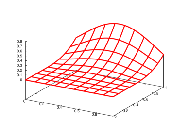
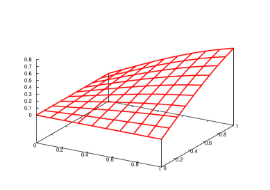
where 𝒳=]0,1[×]0,1[\mathcal{X}=]0,1[\times]0,1[ is the unit square, 𝒜={a2|a21}𝒜conditional-set𝑎superscript2subscriptnorm𝑎21\mathcal{A}=\left\{{a\in\mathds{R}^{2}\,|\,\left\|{a}\right\|_{2}\leq 1}\right\}, =2superscript2\mathcal{B}=\mathds{R}^{2}, ψ1(x1,x2)=sin(x1)×sin(x2)subscript𝜓1subscript𝑥1subscript𝑥2subscript𝑥1subscript𝑥2\psi_{1}(x_{1},x_{2})=\sin(x_{1})\times\sin(x_{2}) for (x1,x2)𝒳subscript𝑥1subscript𝑥2𝒳(x_{1},x_{2})\in\partial\mathcal{X}, and f(x)=(Δu(x)+u(x)20.5u(x)22λu(x))𝑓𝑥Δ𝑢𝑥subscriptnorm𝑢𝑥20.5superscriptsubscriptnorm𝑢𝑥22𝜆𝑢𝑥f(x)=-(\Delta u(x)+\left\|{\nabla u(x)}\right\|_{2}-0.5\left\|{\nabla u(x)}\right\|_{2}^{2}-\lambda u(x)) with u(x1,x2)=sin(x1)×sin(x2)𝑢subscript𝑥1subscript𝑥2subscript𝑥1subscript𝑥2u(x_{1},x_{2})=\sin(x_{1})\times\sin(x_{2}) for x=(x1,x2)𝒳𝑥subscript𝑥1subscript𝑥2𝒳x=(x_{1},x_{2})\in\mathcal{X}. Note that the exact solution is v(x1,x2)=sin(x1)×sin(x2)𝑣subscript𝑥1subscript𝑥2subscript𝑥1subscript𝑥2v(x_{1},x_{2})=\sin(x_{1})\times\sin(x_{2}) on 𝒳=[0,1]×[0,1]𝒳0101\mathcal{X}=[0,1]\times[0,1] and is represented in Figure 3. Indeed, by convex duality (or computation of Fenchel-Legendre transformations [52]), we have that

u2=maxa21,adau and 12u22=maxbdbu12b22formulae-sequencesubscriptnorm𝑢2subscriptformulae-sequencesubscriptnorm𝑎21𝑎superscript𝑑𝑎𝑢 and 12subscriptsuperscriptnorm𝑢22subscript𝑏superscript𝑑𝑏𝑢12subscriptsuperscriptnorm𝑏22\left\|{u}\right\|_{2}=\max_{{\left\|{a}\right\|}_{2}\leq 1,a\in\mathds{R}^{d}}\,a\,\cdot\,\,u\qquad\text{ and }\qquad\frac{1}{2}\left\|{u}\right\|^{2}_{2}=\max_{b\in\mathds{R}^{d}}\,b\,\cdot\,u-\frac{1}{2}\left\|{b}\right\|^{2}_{2}

for all ud𝑢superscript𝑑u\in\mathds{R}^{d}, a=uu22𝑎𝑢superscriptsubscriptnorm𝑢22a=\frac{u}{\left\|{u}\right\|_{2}^{2}} and b=u𝑏𝑢b=u are optimal solutions in these equations.
Refer to caption
Figure 3: Graph of sin(x1)×sin(x2)subscript𝑥1subscript𝑥2\sin(x_{1})\times\sin(x_{2}) on 𝒳=[0,1]×[0,1]𝒳0101\mathcal{X}=[0,1]\times[0,1].

To solve Equation (23), we first discretize the domain [0,1]×[0,1]0101[0,1]\times[0,1] on a grid with m+1𝑚1m+1 points in each direction, i.e. with a discretization step h=1m1𝑚h=\frac{1}{m} and we obtain a discrete space 𝒳hsubscript𝒳\mathcal{X}_{h} with boundary 𝒳hsubscript𝒳\partial\mathcal{X}_{h}. We denote by xi=ihsubscript𝑥𝑖𝑖x_{i}=ih with i=0,,m𝑖0𝑚i=0,\dots,m such that 𝒳h={(xi,xj)|i,j{1,,m1}}subscript𝒳conditional-setsubscript𝑥𝑖subscript𝑥𝑗𝑖𝑗1𝑚1\mathcal{X}_{h}=\left\{{(x_{i},x_{j})\,|\,i,j\in\left\{{1,\dots,m-1}\right\}}\right\} and 𝒳h={(xi,xj)|i{0,m},j{0,,m} or j{0,m},i{0,,m}}subscript𝒳conditional-setsubscript𝑥𝑖subscript𝑥𝑗formulae-sequenceformulae-sequence𝑖0𝑚𝑗0𝑚 or 𝑗0𝑚𝑖0𝑚\partial\mathcal{X}_{h}=\left\{{(x_{i},x_{j})\,|\,i\in\left\{{0,m}\right\},j\in\left\{{0,\dots,m}\right\}\text{ or }j\in\left\{{0,m}\right\},i\in\left\{{0,\dots,m}\right\}}\right\}. Then, using the discretization scheme (16)- (17), Equation (23) becomes for (xi,xj)𝒳hsubscript𝑥𝑖subscript𝑥𝑗subscript𝒳(x_{i},x_{j})\in\mathcal{X}_{h} :

0=0absent\displaystyle 0\,= max(a1,a2)𝒜min(b1,b2){(4v(xi,xj)+v(xi+1,xj)+v(xi1,xj)+v(xi,xj+1)+v(xi,xj1)h2)\displaystyle\max_{(a_{1},a_{2})\in\mathcal{A}}\min_{(b_{1},b_{2})\in\mathcal{B}}\ \Bigg{\{}\left(\frac{-4v(x_{i},x_{j})+v(x_{i+1},x_{j})+v(x_{i-1},x_{j})+v(x_{i},x_{j+1})+v(x_{i},x_{j-1})}{h^{2}}\right)
+(a1b1)(v(xi+1,xj)v(xi,xj)h)1I(a1b1)0+(a1b1)(v(xi,xj)v(xi1,xj)h)1I(a1b1)<0subscript𝑎1subscript𝑏1𝑣subscript𝑥𝑖1subscript𝑥𝑗𝑣subscript𝑥𝑖subscript𝑥𝑗1subscriptIsubscript𝑎1subscript𝑏10subscript𝑎1subscript𝑏1𝑣subscript𝑥𝑖subscript𝑥𝑗𝑣subscript𝑥𝑖1subscript𝑥𝑗1subscriptIsubscript𝑎1subscript𝑏10\displaystyle+(a_{1}-b_{1})\left(\frac{v(x_{i+1},x_{j})-v(x_{i},x_{j})}{h}\right){1{\hskip-2.5pt}\hbox{I}}_{(a_{1}-b_{1})\geq 0}+(a_{1}-b_{1})\left(\frac{v(x_{i},x_{j})-v(x_{i-1},x_{j})}{h}\right){1{\hskip-2.5pt}\hbox{I}}_{(a_{1}-b_{1})<0}
+(a2b2)(v(xi,xj+1)v(xi,xj)h)1I(a2b2)0+(a2b2)(v(xi,xj)v(xi,xj1)h)1I(a2b2)<0subscript𝑎2subscript𝑏2𝑣subscript𝑥𝑖subscript𝑥𝑗1𝑣subscript𝑥𝑖subscript𝑥𝑗1subscriptIsubscript𝑎2subscript𝑏20subscript𝑎2subscript𝑏2𝑣subscript𝑥𝑖subscript𝑥𝑗𝑣subscript𝑥𝑖subscript𝑥𝑗11subscriptIsubscript𝑎2subscript𝑏20\displaystyle+(a_{2}-b_{2})\left(\frac{v(x_{i},x_{j+1})-v(x_{i},x_{j})}{h}\right){1{\hskip-2.5pt}\hbox{I}}_{(a_{2}-b_{2})\geq 0}+(a_{2}-b_{2})\left(\frac{v(x_{i},x_{j})-v(x_{i},x_{j-1})}{h}\right){1{\hskip-2.5pt}\hbox{I}}_{(a_{2}-b_{2})<0}
λv(xi,xj)+b12+b222+f(xi,xj)},\displaystyle-\lambda v(x_{i},x_{j})+\frac{b_{1}^{2}+b_{2}^{2}}{2}+f(x_{i},x_{j})\Bigg{\}}\enspace,

multiply by h2csuperscript2𝑐\frac{h^{2}}{c}, where c=4+h|a1b1|+h|a2b2|>0𝑐4subscript𝑎1subscript𝑏1subscript𝑎2subscript𝑏20c=4+h\left|{a_{1}-b_{1}}\right|+h\left|{a_{2}-b_{2}}\right|>0, and adding v(xi,xj)𝑣subscript𝑥𝑖subscript𝑥𝑗v(x_{i},x_{j}) on both sides, we obtain :

v(xi,xj)=𝑣subscript𝑥𝑖subscript𝑥𝑗absent\displaystyle v(x_{i},x_{j})\,= max(a1,a2)𝒜min(b1,b2)(1+h2cλ)1\displaystyle\max_{(a_{1},a_{2})\in\mathcal{A}}\min_{(b_{1},b_{2})\in\mathcal{B}}\ \left(1+\frac{h^{2}}{c}\lambda\right)^{-1}
{(1c+hc(a1b1)1I(a1b1)0)v(xi+1,xj)+(1chc(a1b1)1I(a1b1)<0)v(xi1,xj)\displaystyle\Bigg{\{}\left(\frac{1}{c}+\frac{h}{c}(a_{1}-b_{1}){1{\hskip-2.5pt}\hbox{I}}_{(a_{1}-b_{1})\geq 0}\right)v(x_{i+1},x_{j})+\left(\frac{1}{c}-\frac{h}{c}(a_{1}-b_{1}){1{\hskip-2.5pt}\hbox{I}}_{(a_{1}-b_{1})<0}\right)v(x_{i-1},x_{j})
+(1c+hc(a2b2)1I(a2b2)0)v(xi,xj+1)+(1chc(a2b2)1I(a2b2)<0)v(xi,xj1)1𝑐𝑐subscript𝑎2subscript𝑏21subscriptIsubscript𝑎2subscript𝑏20𝑣subscript𝑥𝑖subscript𝑥𝑗11𝑐𝑐subscript𝑎2subscript𝑏21subscriptIsubscript𝑎2subscript𝑏20𝑣subscript𝑥𝑖subscript𝑥𝑗1\displaystyle+\left(\frac{1}{c}+\frac{h}{c}(a_{2}-b_{2}){1{\hskip-2.5pt}\hbox{I}}_{(a_{2}-b_{2})\geq 0}\right)v(x_{i},x_{j+1})+\left(\frac{1}{c}-\frac{h}{c}(a_{2}-b_{2}){1{\hskip-2.5pt}\hbox{I}}_{(a_{2}-b_{2})<0}\right)v(x_{i},x_{j-1})
+h2cb12+b222+h2cf(xi,xj)} for (xi,xj)𝒳h,\displaystyle+\frac{h^{2}}{c}\,\frac{b_{1}^{2}+b_{2}^{2}}{2}+\frac{h^{2}}{c}\,f(x_{i},x_{j})\ \Bigg{\}}\qquad\text{ for }(x_{i},x_{j})\in\mathcal{X}_{h}\enspace, (24)

where v(xi,xj)𝑣subscript𝑥𝑖subscript𝑥𝑗v(x_{i},x_{j}) is replaced by ψ1(xi,xj)subscript𝜓1subscript𝑥𝑖subscript𝑥𝑗\psi_{1}(x_{i},x_{j}) for (xi,xj)𝒳hsubscript𝑥𝑖subscript𝑥𝑗subscript𝒳(x_{i},x_{j})\in\partial\mathcal{X}_{h}. This equation has the form of Equation (5) with a discount factor μ𝜇\mu equal to (1+h2cλ)11superscript1superscript2𝑐𝜆11(1+\frac{h^{2}}{c}\lambda)^{-1}\leq 1, transition probabilities from (xi,xj)𝒳hsubscript𝑥𝑖subscript𝑥𝑗subscript𝒳(x_{i},x_{j})\in\mathcal{X}_{h} to (xi,xj)𝒳hsubscript𝑥superscript𝑖subscript𝑥superscript𝑗subscript𝒳(x_{i^{{}^{\prime}}},x_{j^{{}^{\prime}}})\in\mathcal{X}_{h} are given by :

p((xi,xj)|(xi,xj),(a1,a2),(b1,b2))=𝑝conditionalsubscript𝑥superscript𝑖subscript𝑥superscript𝑗subscript𝑥𝑖subscript𝑥𝑗subscript𝑎1subscript𝑎2subscript𝑏1subscript𝑏2absent\displaystyle p((x_{i^{{}^{\prime}}},x_{j^{{}^{\prime}}})|(x_{i},x_{j}),(a_{1},a_{2}),(b_{1},b_{2}))\,=\, 1c+hc(a1b1)1I(a1b1)01𝑐𝑐subscript𝑎1subscript𝑏11subscriptIsubscript𝑎1subscript𝑏10\displaystyle\frac{1}{c}+\frac{h}{c}(a_{1}-b_{1}){1{\hskip-2.5pt}\hbox{I}}_{(a_{1}-b_{1})\geq 0} if i=i+1,j=j,formulae-sequenceif superscript𝑖𝑖1superscript𝑗𝑗\displaystyle\text{ if }i^{{}^{\prime}}=i+1,j^{{}^{\prime}}=j\enspace, (25)
1chc(a1b1)1I(a1b1)<01𝑐𝑐subscript𝑎1subscript𝑏11subscriptIsubscript𝑎1subscript𝑏10\displaystyle\frac{1}{c}-\frac{h}{c}(a_{1}-b_{1}){1{\hskip-2.5pt}\hbox{I}}_{(a_{1}-b_{1})<0} if i=i1,j=j,formulae-sequenceif superscript𝑖𝑖1superscript𝑗𝑗\displaystyle\text{ if }i^{{}^{\prime}}=i-1,j^{{}^{\prime}}=j\enspace,
1c+hc(a2b2)1I(a2b2)01𝑐𝑐subscript𝑎2subscript𝑏21subscriptIsubscript𝑎2subscript𝑏20\displaystyle\frac{1}{c}+\frac{h}{c}(a_{2}-b_{2}){1{\hskip-2.5pt}\hbox{I}}_{(a_{2}-b_{2})\geq 0} if i=i,j=j+1,formulae-sequenceif superscript𝑖𝑖superscript𝑗𝑗1\displaystyle\text{ if }i^{{}^{\prime}}=i,j^{{}^{\prime}}=j+1\enspace,
1chc(a2b2)1I(a2b2)<01𝑐𝑐subscript𝑎2subscript𝑏21subscriptIsubscript𝑎2subscript𝑏20\displaystyle\frac{1}{c}-\frac{h}{c}(a_{2}-b_{2}){1{\hskip-2.5pt}\hbox{I}}_{(a_{2}-b_{2})<0} if i=i,j=j1,formulae-sequenceif superscript𝑖𝑖superscript𝑗𝑗1\displaystyle\text{ if }i^{{}^{\prime}}=i,j^{{}^{\prime}}=j-1\enspace,
00\displaystyle 0 else,else\displaystyle\text{ else}\enspace,

and the running cost is, for (xi,xj)𝒳hsubscript𝑥𝑖subscript𝑥𝑗subscript𝒳(x_{i},x_{j})\in\mathcal{X}_{h} :

r((xi,xj),(a1,a2),(b1,b2))=𝑟subscript𝑥𝑖subscript𝑥𝑗subscript𝑎1subscript𝑎2subscript𝑏1subscript𝑏2absent\displaystyle r((x_{i},x_{j}),(a_{1},a_{2}),(b_{1},b_{2}))\,= h2c(b12+b222+f(xi,xj))superscript2𝑐superscriptsubscript𝑏12superscriptsubscript𝑏222𝑓subscript𝑥𝑖subscript𝑥𝑗\displaystyle\,\frac{h^{2}}{c}\left(\frac{b_{1}^{2}+b_{2}^{2}}{2}+f(x_{i},x_{j})\right)
+(hc(a1b1)1I(a1b1)0)ψ1(xi+1,xj)1I(xi+1,xj)𝒳h𝑐subscript𝑎1subscript𝑏11subscriptIsubscript𝑎1subscript𝑏10subscript𝜓1subscript𝑥𝑖1subscript𝑥𝑗1subscriptIsubscript𝑥𝑖1subscript𝑥𝑗subscript𝒳\displaystyle+\left(\frac{h}{c}(a_{1}-b_{1}){1{\hskip-2.5pt}\hbox{I}}_{(a_{1}-b_{1})\geq 0}\right)\psi_{1}(x_{i+1},x_{j}){1{\hskip-2.5pt}\hbox{I}}_{(x_{i+1},x_{j})\in\partial\mathcal{X}_{h}}
(hc(a1b1)1I(a1b1)<0)ψ1(xi1,xj)1I(xi1,xj)𝒳h𝑐subscript𝑎1subscript𝑏11subscriptIsubscript𝑎1subscript𝑏10subscript𝜓1subscript𝑥𝑖1subscript𝑥𝑗1subscriptIsubscript𝑥𝑖1subscript𝑥𝑗subscript𝒳\displaystyle-\left(\frac{h}{c}(a_{1}-b_{1}){1{\hskip-2.5pt}\hbox{I}}_{(a_{1}-b_{1})<0}\right)\psi_{1}(x_{i-1},x_{j}){1{\hskip-2.5pt}\hbox{I}}_{(x_{i-1},x_{j})\in\partial\mathcal{X}_{h}}
+(hc(a2b2)1I(a2b2)0)ψ1(xi,xj+1)1I(xi,xj+1)𝒳h𝑐subscript𝑎2subscript𝑏21subscriptIsubscript𝑎2subscript𝑏20subscript𝜓1subscript𝑥𝑖subscript𝑥𝑗11subscriptIsubscript𝑥𝑖subscript𝑥𝑗1subscript𝒳\displaystyle+\left(\frac{h}{c}(a_{2}-b_{2}){1{\hskip-2.5pt}\hbox{I}}_{(a_{2}-b_{2})\geq 0}\right)\psi_{1}(x_{i},x_{j+1}){1{\hskip-2.5pt}\hbox{I}}_{(x_{i},x_{j+1})\in\partial\mathcal{X}_{h}}
(hc(a2b2)1I(a2b2)<0)ψ1(xi,xj1)1I(xi,xj1)𝒳h.𝑐subscript𝑎2subscript𝑏21subscriptIsubscript𝑎2subscript𝑏20subscript𝜓1subscript𝑥𝑖subscript𝑥𝑗11subscriptIsubscript𝑥𝑖subscript𝑥𝑗1subscript𝒳\displaystyle-\left(\frac{h}{c}(a_{2}-b_{2}){1{\hskip-2.5pt}\hbox{I}}_{(a_{2}-b_{2})<0}\right)\psi_{1}(x_{i},x_{j-1}){1{\hskip-2.5pt}\hbox{I}}_{(x_{i},x_{j-1})\in\partial\mathcal{X}_{h}}\enspace.

Note that when i,j{2,,m2}𝑖𝑗2𝑚2i,j\in\{2,\dots,m-2\} the sum of the transition probabilities from (xi,xj)subscript𝑥𝑖subscript𝑥𝑗(x_{i},x_{j}) to the points of 𝒳hsubscript𝒳\mathcal{X}_{h} equals μ𝜇\mu, when i𝑖i or j𝑗j is in {1,m1}1𝑚1\{1,m-1\} this sum is strictly less than μ𝜇\mu. Hence, the matrix Mα,βsuperscript𝑀𝛼𝛽M^{{\alpha},{\beta}} in (21) is substochastic, and since it is irreducible, it has a spectral radius strictly less than one. So even when λ=0𝜆0\lambda=0 or equivalently μ=1𝜇1\mu=1, the system (21) has an unique solution and the dynamic programing equations has also an unique solution. Hence, we shall take λ=0𝜆0\lambda=0 in the numerical tests. Note also that for this example, the matrices Mα,βsuperscript𝑀𝛼𝛽M^{{\alpha},{\beta}} in (21) are not symmetric but close to be symmetric when hh is small, since the non-symmetric part correspond to the order one term in equation (24) and are dominated by order two terms when b𝑏b is optimal in (24).

Table 1: Numerical results for equation (23) on a 1025×1025102510251025\times 1025 points grid.
Policy iteration with LU
s𝑠{s} kmax𝑘𝑚𝑎𝑥{{k}max} rvsubscriptnormsubscript𝑟𝑣\left\|{r_{v}}\right\|_{\infty} rvL2subscriptnormsubscript𝑟𝑣subscript𝐿2\left\|{r_{v}}\right\|_{L_{2}} esubscriptnorm𝑒\left\|{e}\right\|_{\infty} eL2subscriptnorm𝑒subscript𝐿2\left\|{e}\right\|_{L_{2}} cpu time (s)
111 333 8.51e78.51𝑒78.51e-7 5.96e75.96𝑒75.96e-7 4.47e24.47𝑒24.47e-2 2.48e22.48𝑒22.48e-2 1.40e+21.40𝑒21.40e+2
222 222 2.44e82.44𝑒82.44e-8 6.16e96.16𝑒96.16e-9 1.84e41.84𝑒41.84e-4 1.05e41.05𝑒41.05e-4 2.31e+22.31𝑒22.31e+2
333 111 7.38e137.38𝑒137.38e-13 2.03e132.03𝑒132.03e-13 4.13e64.13𝑒64.13e-6 2.16e62.16𝑒62.16e-6 2.77e+22.77𝑒22.77e+2
AMGπ𝜋\pi
s𝑠{s} kmax𝑘𝑚𝑎𝑥{{k}max} rvsubscriptnormsubscript𝑟𝑣\left\|{r_{v}}\right\|_{\infty} rvL2subscriptnormsubscript𝑟𝑣subscript𝐿2\left\|{r_{v}}\right\|_{L_{2}} esubscriptnorm𝑒\left\|{e}\right\|_{\infty} eL2subscriptnorm𝑒subscript𝐿2\left\|{e}\right\|_{L_{2}} cpu time (s)
111 333 8.51e78.51𝑒78.51e-7 5.96e75.96𝑒75.96e-7 4.47e24.47𝑒24.47e-2 2.48e22.48𝑒22.48e-2 2.65e+12.65𝑒12.65e+1
222 222 2.44e82.44𝑒82.44e-8 6.16e96.16𝑒96.16e-9 1.84e41.84𝑒41.84e-4 1.05e41.05𝑒41.05e-4 4.59e+14.59𝑒14.59e+1
333 111 7.92e137.92𝑒137.92e-13 2.02e132.02𝑒132.02e-13 4.13e64.13𝑒64.13e-6 2.16e62.16𝑒62.16e-6 5.56e+15.56𝑒15.56e+1

In tables 1, we present numerical results when equations (23) is discretized on a grid with 102510251025 points in each direction, i.e. with a discretization step of h=1/2101superscript210h=1/2^{10}. The stopping criterion for the policy iterations is ϵ=1010italic-ϵsuperscript1010\epsilon=10^{-10}. The first table of 1 shows the results of the policy iteration algorithm with a direct solver LU (we used the package UMFPACK [21]) and the second table of 1 the results of AMGπ𝜋\pi. We observe that AMGπ𝜋\pi solves the problem faster than the policy iterations with a direct solver. In both tables, we see that only three steps on max policies are needed (first column) and a total of six steps on min policies (second column) which involves the resolution of six linear systems. The small number of iterations is due to the fact that the solution is regular. In table 2, we show that the computation time is improved when applying FAMGπ𝜋\pi with c=0.1𝑐0.1c=0.1 to the same example. In this case, the problem is solved in approximately 18s18𝑠18s.

Table 2: Numerical results for Equation (23) on a 1025×1025102510251025\times 1025 points grid, computed by FAMGπ𝜋\pi with c=101𝑐superscript101c=10^{-1}.
s𝑠{s} kmax𝑘𝑚𝑎𝑥{{k}max} rvsubscriptnormsubscript𝑟𝑣\left\|{r_{v}}\right\|_{\infty} rvL2subscriptnormsubscript𝑟𝑣subscript𝐿2\left\|{r_{v}}\right\|_{L_{2}} esubscriptnorm𝑒\left\|{e}\right\|_{\infty} eL2subscriptnorm𝑒subscript𝐿2\left\|{e}\right\|_{L_{2}} cpu time (s)
points in each direction : 333, h 5.00e015.00𝑒015.00e-01
111 222 1.42e011.42𝑒011.42e-01 1.42e011.42𝑒011.42e-01 1.07e011.07𝑒011.07e-01 1.07e011.07𝑒011.07e-01 <<1much-less-thanabsent1<<1
222 111 2.34e032.34𝑒032.34e-03 2.34e032.34𝑒032.34e-03 2.45e042.45𝑒042.45e-04 2.45e042.45𝑒042.45e-04 <<1much-less-thanabsent1<<1
points in each direction : 555, h 2.50e012.50𝑒012.50e-01
111 222 5.53e035.53𝑒035.53e-03 2.84e032.84𝑒032.84e-03 3.00e033.00𝑒033.00e-03 1.75e031.75𝑒031.75e-03 <<1much-less-thanabsent1<<1
points in each direction : 999, h 1.25e011.25𝑒011.25e-01
111 222 2.40e042.40𝑒042.40e-04 1.10e041.10𝑒041.10e-04 8.20e048.20𝑒048.20e-04 4.46e044.46𝑒044.46e-04 <<1much-less-thanabsent1<<1
points in each direction : 171717, h 6.25e026.25𝑒026.25e-02
111 222 3.18e053.18𝑒053.18e-05 7.83e067.83𝑒067.83e-06 3.36e043.36𝑒043.36e-04 1.90e041.90𝑒041.90e-04 1.00e021.00𝑒021.00e-02
points in each direction : 333333, h 3.12e023.12𝑒023.12e-02
111 111 5.89e045.89𝑒045.89e-04 7.08e057.08𝑒057.08e-05 5.05e045.05𝑒045.05e-04 1.99e041.99𝑒041.99e-04 1.00e021.00𝑒021.00e-02
points in each direction : 656565, h 1.56e021.56𝑒021.56e-02
111 111 1.69e041.69𝑒041.69e-04 1.25e051.25𝑒051.25e-05 1.62e041.62𝑒041.62e-04 4.67e054.67𝑒054.67e-05 4.00e024.00𝑒024.00e-02
points in each direction : 129129129, h 7.81e037.81𝑒037.81e-03
111 111 4.28e054.28𝑒054.28e-05 2.16e062.16𝑒062.16e-06 4.73e054.73𝑒054.73e-05 1.21e051.21𝑒051.21e-05 1.80e011.80𝑒011.80e-01
points in each direction : 257257257, h 3.91e033.91𝑒033.91e-03
111 111 1.08e051.08𝑒051.08e-05 3.77e073.77𝑒073.77e-07 1.31e051.31𝑒051.31e-05 6.07e066.07𝑒066.07e-06 7.50e017.50𝑒017.50e-01
points in each direction : 513513513, h 1.95e031.95𝑒031.95e-03
111 111 2.70e062.70𝑒062.70e-06 6.61e086.61𝑒086.61e-08 7.29e067.29𝑒067.29e-06 3.56e063.56𝑒063.56e-06 3.13e+003.13𝑒003.13e+00
points in each direction : 102510251025, h 9.77e049.77𝑒049.77e-04
111 222 1.23e101.23𝑒101.23e-10 8.13e138.13𝑒138.13e-13 4.16e064.16𝑒064.16e-06 2.17e062.17𝑒062.17e-06 1.85e+011.85𝑒011.85e+01
02004006008001000120014002002superscript2002200^{2}4002superscript4002400^{2}6002superscript6002600^{2}8002superscript8002800^{2}10002superscript100021000^{2}12002superscript120021200^{2}14002superscript140021400^{2}

CPU time (seconds)

number of discretization nodesRefer to captionPI with LU (UMFPACK)PI with AMG
Figure 4: Comparison between AMGπ𝜋\pi versus policy iteration algorithm with a LU solver for solving equation (23) when increasing the size of the problem.
681012142002superscript2002200^{2}4002superscript4002400^{2}6002superscript6002600^{2}8002superscript8002800^{2}10002superscript100021000^{2}12002superscript120021200^{2}14002superscript140021400^{2}

Total number of linear systems solved

number of discretization nodesRefer to caption
Figure 5: Number of iterations on min policies (i.e the number of linear systems solved) for solving equation (23) when increasing the size of the problem corresponding to figure 4 for both methods (AMGπ𝜋\pi and policy iteration algorithm with LU).

In figure 4, we compare the policy iteration algorithm with a direct solver LU (UMFPACK [21]) and AMGπ𝜋\pi for solving equation (24), when increasing by one the number of discretization points in each direction from m=5𝑚5m=5 to m=1500𝑚1500m=1500. The stopping criterion for the policy iterations is ϵ=1010italic-ϵsuperscript1010\epsilon=10^{-10}. In figure 5, we represent the corresponding number of iterations on min policies, i.e the number of linear systems solved for each size of problem, this number is the same for both methods. We can see that the most part of the computation time for the resolution of the non-linear equation (24) is used to solved the linear systems involved in the policy iteration. We also remark that the computation time for AMGπ𝜋\pi seems to grow linearly with the size of the problem.

s𝑠{s} kmax𝑘𝑚𝑎𝑥{{k}max} AMG rvsubscriptnormsubscript𝑟𝑣\left\|{r_{v}}\right\|_{\infty} rvL2subscriptnormsubscript𝑟𝑣subscript𝐿2\left\|{r_{v}}\right\|_{L_{2}} esubscriptnorm𝑒\left\|{e}\right\|_{\infty} eL2subscriptnorm𝑒subscript𝐿2\left\|{e}\right\|_{L_{2}} cpu time (s)
111 222 5,4545,4 2.15e042.15𝑒042.15e-04 1.52e041.52𝑒041.52e-04 4.45e024.45𝑒024.45e-02 2.50e022.50𝑒022.50e-02 5.00e025.00𝑒025.00e-02
222 222 4,3434,3 5.97e065.97𝑒065.97e-06 1.59e061.59𝑒061.59e-06 2.36e042.36𝑒042.36e-04 1.43e041.43𝑒041.43e-04 1.00e011.00𝑒011.00e-01
333 111 333 3.02e093.02𝑒093.02e-09 7.47e107.47𝑒107.47e-10 6.49e056.49𝑒056.49e-05 3.44e053.44𝑒053.44e-05 1.30e011.30𝑒011.30e-01
Table 3: Numerical results with a 65×65656565\times 65 points grid, computed by AMGπ𝜋\pi for equation (23).
s𝑠{s} kmax𝑘𝑚𝑎𝑥{{k}max} AMG rvsubscriptnormsubscript𝑟𝑣\left\|{r_{v}}\right\|_{\infty} rvL2subscriptnormsubscript𝑟𝑣subscript𝐿2\left\|{r_{v}}\right\|_{L_{2}} esubscriptnorm𝑒\left\|{e}\right\|_{\infty} eL2subscriptnorm𝑒subscript𝐿2\left\|{e}\right\|_{L_{2}} cpu time (s)
111 222 5,4545,4 5.40e055.40𝑒055.40e-05 3.80e053.80𝑒053.80e-05 4.46e024.46𝑒024.46e-02 2.49e022.49𝑒022.49e-02 2.30e012.30𝑒012.30e-01
222 222 4,3434,3 1.53e061.53𝑒061.53e-06 3.95e073.95𝑒073.95e-07 2.07e042.07𝑒042.07e-04 1.23e041.23𝑒041.23e-04 4.30e014.30𝑒014.30e-01
333 111 333 4.08e104.08𝑒104.08e-10 9.65e119.65𝑒119.65e-11 3.28e053.28𝑒053.28e-05 1.72e051.72𝑒051.72e-05 5.40e015.40𝑒015.40e-01
Table 4: Numerical results with a 129×129129129129\times 129 points grid, computed by AMGπ𝜋\pi for equation (23).
s𝑠{s} kmax𝑘𝑚𝑎𝑥{{k}max} AMG rvsubscriptnormsubscript𝑟𝑣\left\|{r_{v}}\right\|_{\infty} rvL2subscriptnormsubscript𝑟𝑣subscript𝐿2\left\|{r_{v}}\right\|_{L_{2}} esubscriptnorm𝑒\left\|{e}\right\|_{\infty} eL2subscriptnorm𝑒subscript𝐿2\left\|{e}\right\|_{L_{2}} cpu time (s)
111 222 5,4545,4 1.35e051.35𝑒051.35e-05 9.51e069.51𝑒069.51e-06 4.47e024.47𝑒024.47e-02 2.49e022.49𝑒022.49e-02 1.06e+001.06𝑒001.06e+00
222 222 4,3434,3 3.86e073.86𝑒073.86e-07 9.86e089.86𝑒089.86e-08 1.94e041.94𝑒041.94e-04 1.13e041.13𝑒041.13e-04 1.98e+001.98𝑒001.98e+00
333 111 333 5.17e115.17𝑒115.17e-11 1.22e111.22𝑒111.22e-11 1.65e051.65𝑒051.65e-05 8.63e068.63𝑒068.63e-06 2.49e+002.49𝑒002.49e+00
Table 5: Numerical results with a 257×257257257257\times 257 points grid, computed by AMGπ𝜋\pi for equation (23).
s𝑠{s} kmax𝑘𝑚𝑎𝑥{{k}max} AMG rvsubscriptnormsubscript𝑟𝑣\left\|{r_{v}}\right\|_{\infty} rvL2subscriptnormsubscript𝑟𝑣subscript𝐿2\left\|{r_{v}}\right\|_{L_{2}} esubscriptnorm𝑒\left\|{e}\right\|_{\infty} eL2subscriptnorm𝑒subscript𝐿2\left\|{e}\right\|_{L_{2}} cpu time (s)
111 222 5,4545,4 3.39e063.39𝑒063.39e-06 2.38e062.38𝑒062.38e-06 4.47e024.47𝑒024.47e-02 2.48e022.48𝑒022.48e-02 4.55e+004.55𝑒004.55e+00
222 222 4,3434,3 9.71e089.71𝑒089.71e-08 2.46e082.46𝑒082.46e-08 1.87e041.87𝑒041.87e-04 1.08e041.08𝑒041.08e-04 8.28e+008.28𝑒008.28e+00
333 111 333 6.26e126.26𝑒126.26e-12 1.55e121.55𝑒121.55e-12 8.26e068.26𝑒068.26e-06 4.31e064.31𝑒064.31e-06 1.04e+011.04𝑒011.04e+01
Table 6: Numerical results with a 513×513513513513\times 513 points grid, computed by AMGπ𝜋\pi for equation (23).
s𝑠{s} kmax𝑘𝑚𝑎𝑥{{k}max} AMG rvsubscriptnormsubscript𝑟𝑣\left\|{r_{v}}\right\|_{\infty} rvL2subscriptnormsubscript𝑟𝑣subscript𝐿2\left\|{r_{v}}\right\|_{L_{2}} esubscriptnorm𝑒\left\|{e}\right\|_{\infty} eL2subscriptnorm𝑒subscript𝐿2\left\|{e}\right\|_{L_{2}} cpu time (s)
111 222 5,4545,4 8.48e078.48𝑒078.48e-07 5.95e075.95𝑒075.95e-07 4.47e024.47𝑒024.47e-02 2.48e022.48𝑒022.48e-02 1.85e+011.85𝑒011.85e+01
222 222 4,3434,3 2.43e082.43𝑒082.43e-08 6.15e096.15𝑒096.15e-09 1.83e041.83𝑒041.83e-04 1.05e041.05𝑒041.05e-04 3.40e+013.40𝑒013.40e+01
333 111 333 7.40e137.40𝑒137.40e-13 2.02e132.02𝑒132.02e-13 4.13e064.13𝑒064.13e-06 2.16e062.16𝑒062.16e-06 4.27e+014.27𝑒014.27e+01
Table 7: Numerical results with a 1025×1025102510251025\times 1025 points grid, computed by AMGπ𝜋\pi for equation (23).
s𝑠{s} kmax𝑘𝑚𝑎𝑥{{k}max} AMG rvsubscriptnormsubscript𝑟𝑣\left\|{r_{v}}\right\|_{\infty} rvL2subscriptnormsubscript𝑟𝑣subscript𝐿2\left\|{r_{v}}\right\|_{L_{2}} esubscriptnorm𝑒\left\|{e}\right\|_{\infty} eL2subscriptnorm𝑒subscript𝐿2\left\|{e}\right\|_{L_{2}} cpu time (s)
111 222 5,4545,4 2.12e072.12𝑒072.12e-07 1.49e071.49𝑒071.49e-07 4.47e024.47𝑒024.47e-02 2.48e022.48𝑒022.48e-02 7.46e+017.46𝑒017.46e+01
222 222 4,3434,3 6.09e096.09𝑒096.09e-09 1.54e091.54𝑒091.54e-09 1.82e041.82𝑒041.82e-04 1.04e041.04𝑒041.04e-04 1.38e+021.38𝑒021.38e+02
333 111 333 1.13e131.13𝑒131.13e-13 3.04e143.04𝑒143.04e-14 2.07e062.07𝑒062.07e-06 1.08e061.08𝑒061.08e-06 1.72e+021.72𝑒021.72e+02
Table 8: Numerical results with a 2049×2049204920492049\times 2049 points grid, computed by AMGπ𝜋\pi for equation (23).

Each table 8 to 8 contains numerical results for Equation (23) discretized on grids with discretization step h=1261superscript26h=\frac{1}{2^{6}}, h=1271superscript27h=\frac{1}{2^{7}}, h=1281superscript28h=\frac{1}{2^{8}}, h=1291superscript29h=\frac{1}{2^{9}}, h=12101superscript210h=\frac{1}{2^{10}} and h=12111superscript211h=\frac{1}{2^{11}} respectively. For these tests, the stopping criterion for the policy iterations is ϵ=0.001h2italic-ϵ0.001superscript2\epsilon=0.001\,{h}^{2} where hh is the discretization step. The stopping criterion for the linear solver AMG is r2<1012subscriptnorm𝑟2superscript1012\left\|{r}\right\|_{2}<10^{-12} where r𝑟r is the residual for the linear system. For each line of the tables, the third column, named AMG, contains the number of iterations needed by AMG for solving each linear system (kmax𝑘𝑚𝑎𝑥{{k}max} systems per line). We can see that the number of iterations of AMG is independent of the size of the problem. Note that the norm of the error enorm𝑒\left\|{e}\right\| decrease slowly when the grid becomes finer, this is because the exact solution (Figure 3) is smooth and a small number of points is sufficient to get a good approximation, also the non-linearity of the problem gives a worse approximation than one might expect in the linear case. But a smooth solution is generally more difficult for linear iterative solvers.

6.2 Optimal stopping game

Next tests concern an optimal stopping time game where the value v:𝒳:𝑣𝒳v:\mathcal{X}\rightarrow\mathds{R} of the game is solution of the variational inequality :

{maxa𝒜{minb(0.5Δv(x)(bv(x))+b222+f(x))\raisebox{-0.6pt}{\hspace*{0.2pt}$1$}⃝,ψ2(x)v(x)\raisebox{-0.6pt}{\hspace*{0.2pt}$2$}⃝}= 0x in 𝒳v(x)=ψ1(x)x in 𝒳casessubscript𝑎𝒜subscriptsubscript𝑏0.5Δ𝑣𝑥𝑏𝑣𝑥subscriptsuperscriptnorm𝑏222𝑓𝑥\raisebox{-0.6pt}{\hspace*{0.2pt}$1$}⃝subscriptsubscript𝜓2𝑥𝑣𝑥\raisebox{-0.6pt}{\hspace*{0.2pt}$2$}⃝ 0𝑥 in 𝒳𝑣𝑥subscript𝜓1𝑥𝑥 in 𝒳\left\{\begin{array}[]{l l}{\displaystyle\max_{a\in\mathcal{A}}\left\{\underbrace{\min_{b\in\mathcal{B}}\left(0.5\Delta v(x)-\left(b\cdot\nabla v(x)\right)+\frac{\left\|{b}\right\|^{2}_{2}}{2}+f(x)\right)}_{\begin{subarray}{c}\text{\tiny\raisebox{-0.6pt}{\hspace*{0.2pt}$1$}⃝}\end{subarray}}\,,\,\underbrace{\psi_{2}(x)-v(x)}_{\begin{subarray}{c}\text{\tiny\raisebox{-0.6pt}{\hspace*{0.2pt}$2$}⃝}\end{subarray}}\right\}\,=\,0}&x\text{ in }\mathcal{X}\\ v(x)=\psi_{1}(x)&x\text{ in }\partial\mathcal{X}\end{array}\right. (26)

where 𝒳=]0,1[×]0,1[\mathcal{X}=]0,1[\times]0,1[ is the unit square, the sets 𝒜={0,1}𝒜01\mathcal{A}=\left\{{0,1}\right\}, =2superscript2\mathcal{B}=\mathds{R}^{2}, ψ2(x1,x2)=0subscript𝜓2subscript𝑥1subscript𝑥20\psi_{2}(x_{1},x_{2})=0 for (x1,x2)𝒳subscript𝑥1subscript𝑥2𝒳(x_{1},x_{2})\in\mathcal{X}, for (x1,x2)𝒳subscript𝑥1subscript𝑥2𝒳(x_{1},x_{2})\in\mathcal{X} :

f(x1,x2)={(0.5Δu(x1,x2)0.5u(x1,x2)22)ifx2(x10.5)2+0.10.5Δu(x1,x2)0.5u(x1,x2)22else,𝑓subscript𝑥1subscript𝑥2cases0.5Δ𝑢subscript𝑥1subscript𝑥20.5superscriptsubscriptnorm𝑢subscript𝑥1subscript𝑥222ifsubscript𝑥2superscriptsubscript𝑥10.520.10.5Δ𝑢subscript𝑥1subscript𝑥20.5superscriptsubscriptnorm𝑢subscript𝑥1subscript𝑥222elsef(x_{1},x_{2})\,=\,\left\{\begin{array}[]{l l}-(0.5\Delta u(x_{1},x_{2})-0.5\left\|{\nabla u(x_{1},x_{2})}\right\|_{2}^{2})&\text{if}\ x_{2}\geq(x_{1}-0.5)^{2}+0.1\\ 0.5\Delta u(x_{1},x_{2})-0.5\left\|{\nabla u(x_{1},x_{2})}\right\|_{2}^{2}&\text{else}\enspace,\\ \end{array}\right.

and for (x1,x2)𝒳subscript𝑥1subscript𝑥2𝒳(x_{1},x_{2})\in\partial\mathcal{X} : ψ1(x1,x2)=u(x1,x2)subscript𝜓1subscript𝑥1subscript𝑥2𝑢subscript𝑥1subscript𝑥2\psi_{1}(x_{1},x_{2})=u(x_{1},x_{2}) where

u(x1,x2)={(x2((x10.5)2+0.1))3ifx2(x10.5)2+0.10else.𝑢subscript𝑥1subscript𝑥2casessuperscriptsubscript𝑥2superscriptsubscript𝑥10.520.13ifsubscript𝑥2superscriptsubscript𝑥10.520.10elseu(x_{1},x_{2})\,=\,\left\{\begin{array}[]{l l}(x_{2}-((x_{1}-0.5)^{2}+0.1))^{3}&\text{if}\ x_{2}\geq(x_{1}-0.5)^{2}+0.1\\ 0&\text{else}\enspace.\end{array}\right.

The definitions of the functions f𝑓f, ψ1subscript𝜓1\psi_{1} and ψ2subscript𝜓2\psi_{2} are chosen such that the function u𝑢u, represented in Figure 6, is solution of (26) almost everywhere and such that the terms \raisebox{-0.9pt}{\hspace*{0.7pt}${1}$}⃝ and \raisebox{-0.9pt}{\hspace*{0.7pt}${2}$}⃝ in Equation (26) are non positive for all x𝒳𝑥𝒳x\in\mathcal{X} (this condition must hold for the variational inequality to be well-defined). This example leads to a free boundary problem for the actions of max. Indeed, the points of the state space 𝒳hsubscript𝒳\mathcal{X}_{h} can be divided in two parts, the points where max chooses action 111 (means continue to play) and the points where max chooses action 00 (means that he stops the game). For (x1,x2)𝒳hsubscript𝑥1subscript𝑥2subscript𝒳(x_{1},x_{2})\in\mathcal{X}_{h}, the optimal strategy α𝛼{\alpha} for max is α(x1,x2)=1𝛼subscript𝑥1subscript𝑥21{\alpha}(x_{1},x_{2})=1 if x2(x10.5)2+0.1subscript𝑥2superscriptsubscript𝑥10.520.1x_{2}\geq(x_{1}-0.5)^{2}+0.1 and α(x1,x2)=0𝛼subscript𝑥1subscript𝑥20{\alpha}(x_{1},x_{2})=0 else, for all (x1,x2)𝒳subscript𝑥1subscript𝑥2𝒳(x_{1},x_{2})\in\mathcal{X}.

As for the previous example, the domain 𝒳𝒳\mathcal{X} is discretized on a grid with m+1𝑚1m+1 points in each direction, i.e. with a discretization step h=1m1𝑚h=\frac{1}{m} and we obtain a discrete space 𝒳hsubscript𝒳\mathcal{X}_{h} with boundary 𝒳hsubscript𝒳\partial\mathcal{X}_{h}. Then, Equation (26) is discretized by using the discretization scheme (16)- (17). After, the equations \raisebox{-0.9pt}{\hspace*{0.7pt}${1}$}⃝ and \raisebox{-0.9pt}{\hspace*{0.7pt}${2}$}⃝ are simplified separately by keeping equations (14) true. In this case, only equation \raisebox{-0.9pt}{\hspace*{0.7pt}${1}$}⃝ is multiply by h2csuperscript2𝑐\frac{h^{2}}{c} with c𝑐c an appropriate constant. After discretization, we obtain the following dynamic programming equation for a game with state space 𝒳hsubscript𝒳\mathcal{X}_{h} :

v(xi,xj)=max{\displaystyle v(x_{i},x_{j})=\quad\max\Bigg{\{} min(b1,b2)(12cb1hc1Ib10)v(xi+1,xj)+(12c+b1hc1Ib1>0)v(xi1,xj)subscriptsubscript𝑏1subscript𝑏212𝑐subscript𝑏1𝑐1subscriptIsubscript𝑏10𝑣subscript𝑥𝑖1subscript𝑥𝑗12𝑐subscript𝑏1𝑐1subscriptIsubscript𝑏10𝑣subscript𝑥𝑖1subscript𝑥𝑗\displaystyle\min_{(b_{1},b_{2})\in\mathcal{B}}\ \left(\frac{1}{2c}-b_{1}\frac{h}{c}{1{\hskip-2.5pt}\hbox{I}}_{b_{1}\leq 0}\right)v(x_{i+1},x_{j})+\left(\frac{1}{2c}+b_{1}\frac{h}{c}{1{\hskip-2.5pt}\hbox{I}}_{b_{1}>0}\right)v(x_{i-1},x_{j})
+(12cb2hc1Ib20)v(xi,xj+1)+(12c+b2hc1Ib2>0)v(xi,xj1)12𝑐subscript𝑏2𝑐1subscriptIsubscript𝑏20𝑣subscript𝑥𝑖subscript𝑥𝑗112𝑐subscript𝑏2𝑐1subscriptIsubscript𝑏20𝑣subscript𝑥𝑖subscript𝑥𝑗1\displaystyle+\left(\frac{1}{2c}-b_{2}\frac{h}{c}{1{\hskip-2.5pt}\hbox{I}}_{b_{2}\leq 0}\right)v(x_{i},x_{j+1})+\left(\frac{1}{2c}+b_{2}\frac{h}{c}{1{\hskip-2.5pt}\hbox{I}}_{b_{2}>0}\right)v(x_{i},x_{j-1})
+h2cb12+b222+h2cf(xi,xj),ψ2(xi,xj)} for (xi,xj)𝒳h\displaystyle+\frac{h^{2}}{c}\,\frac{b_{1}^{2}+b_{2}^{2}}{2}+\frac{h^{2}}{c}\,f(x_{i},x_{j}),\quad\psi_{2}(x_{i},x_{j})\quad\Bigg{\}}\qquad\text{ for }(x_{i},x_{j})\in\mathcal{X}_{h}

with c=2+h|b1|+h|b2|>0𝑐2subscript𝑏1subscript𝑏20c=2+h\left|{b_{1}}\right|+h\left|{b_{2}}\right|>0 and v(xi,xj)=ψ1(xi,xj)𝑣subscript𝑥𝑖subscript𝑥𝑗subscript𝜓1subscript𝑥𝑖subscript𝑥𝑗v(x_{i},x_{j})=\psi_{1}(x_{i},x_{j}) for (xi,xj)𝒳hsubscript𝑥𝑖subscript𝑥𝑗subscript𝒳(x_{i},x_{j})\in\partial\mathcal{X}_{h}. The same comments about non-symmetry and the discount factor in equation (24) hold here. That is λ=0𝜆0\lambda=0 or equivalently μ=1𝜇1\mu=1.

Refer to caption
Figure 6: Graph of the solution of equation (26).
Refer to caption (a) Refer to caption (b)
Refer to caption (c) Refer to caption (d)
Refer to caption (e) Refer to caption (f)
Refer to caption (g)
Figure 7: Application of AMGπ𝜋\pi to the free boundary problem (26) for a 1025×1025102510251025\times 1025 points grid : (a) after 100100100 iterations, (b) after 200200200 iterations, (c) after 300300300 iterations, (d) after 400400400 iterations, (e) after 500500500 iterations, (f) after 600600600 iterations and (g) after 700700700 iterations.
Table 9: Numerical results for optimal stopping time game (26) with a 1025×1025102510251025\times 1025 points grid, computed by AMGπ𝜋\pi with ϵ=1014italic-ϵsuperscript1014\epsilon=10^{-14}.
s𝑠{s} kmax𝑘𝑚𝑎𝑥{{k}max} rvsubscriptnormsubscript𝑟𝑣\left\|{r_{v}}\right\|_{\infty} rvL2subscriptnormsubscript𝑟𝑣subscript𝐿2\left\|{r_{v}}\right\|_{L_{2}} esubscriptnorm𝑒\left\|{e}\right\|_{\infty} eL2subscriptnorm𝑒subscript𝐿2\left\|{e}\right\|_{L_{2}} cpu time (s)
111 00 3.645e013.645𝑒013.645e-01 9.195e039.195𝑒039.195e-03 7.243e017.243𝑒017.243e-01 1.998e011.998𝑒011.998e-01 1.790e+001.790𝑒001.790e+00
222 444 1.497e011.497𝑒011.497e-01 1.347e031.347𝑒031.347e-03 3.782e013.782𝑒013.782e-01 1.218e011.218𝑒011.218e-01 1.376e+011.376𝑒011.376e+01
333 444 1.094e011.094𝑒011.094e-01 8.839e048.839𝑒048.839e-04 3.767e013.767𝑒013.767e-01 1.213e011.213𝑒011.213e-01 2.492e+012.492𝑒012.492e+01
\dots
100100100 333 1.744e021.744𝑒021.744e-02 4.444e054.444𝑒054.444e-05 2.392e012.392𝑒012.392e-01 8.016e028.016𝑒028.016e-02 1.009e+031.009𝑒031.009e+03
\dots
200200200 333 7.398e037.398𝑒037.398e-03 1.879e051.879𝑒051.879e-05 1.222e011.222𝑒011.222e-01 3.996e023.996𝑒023.996e-02 2.214e+032.214𝑒032.214e+03
\dots
300300300 333 2.510e032.510𝑒032.510e-03 8.779e068.779𝑒068.779e-06 5.614e025.614𝑒025.614e-02 1.728e021.728𝑒021.728e-02 3.619e+033.619𝑒033.619e+03
\dots
400400400 222 1.258e031.258𝑒031.258e-03 4.363e064.363𝑒064.363e-06 2.321e022.321𝑒022.321e-02 6.519e036.519𝑒036.519e-03 4.770e+034.770𝑒034.770e+03
\dots
500500500 222 4.761e044.761𝑒044.761e-04 1.620e061.620𝑒061.620e-06 6.601e036.601𝑒036.601e-03 1.532e031.532𝑒031.532e-03 5.861e+035.861𝑒035.861e+03
\dots
600600600 222 8.857e058.857𝑒058.857e-05 2.781e072.781𝑒072.781e-07 7.274e047.274𝑒047.274e-04 9.598e059.598𝑒059.598e-05 7.045e+037.045𝑒037.045e+03
\dots
650650650 222 1.533e051.533𝑒051.533e-05 4.231e084.231𝑒084.231e-08 1.538e041.538𝑒041.538e-04 6.331e056.331𝑒056.331e-05 7.630e+037.630𝑒037.630e+03
\dots
700700700 111 5.647e085.647𝑒085.647e-08 8.734e118.734𝑒118.734e-11 1.571e041.571𝑒041.571e-04 6.619e056.619𝑒056.619e-05 8.134e+038.134𝑒038.134e+03
701701701 111 1.207e081.207𝑒081.207e-08 2.267e112.267𝑒112.267e-11 1.571e041.571𝑒041.571e-04 6.619e056.619𝑒056.619e-05 8.141e+038.141𝑒038.141e+03
702702702 111 9.992e169.992𝑒169.992e-16 7.284e177.284𝑒177.284e-17 1.571e041.571𝑒041.571e-04 6.619e056.619𝑒056.619e-05 8.148e+038.148𝑒038.148e+03
Table 10: Numerical results for optimal stopping time game (26) with a 1025×1025102510251025\times 1025 points grid, computed by FAMGπ𝜋\pi with c=102𝑐superscript102c=10^{-2} and ϵ=1014italic-ϵsuperscript1014\epsilon=10^{-14}.
s𝑠{s} kmax𝑘𝑚𝑎𝑥{{k}max} rvsubscriptnormsubscript𝑟𝑣\left\|{r_{v}}\right\|_{\infty} rvL2subscriptnormsubscript𝑟𝑣subscript𝐿2\left\|{r_{v}}\right\|_{L_{2}} esubscriptnorm𝑒\left\|{e}\right\|_{\infty} eL2subscriptnorm𝑒subscript𝐿2\left\|{e}\right\|_{L_{2}} cpu time (s)
points in each direction : 333, step size : 5.00e015.00𝑒015.00e-01
111 111 2.17e012.17𝑒012.17e-01 2.17e012.17𝑒012.17e-01 1.53e011.53𝑒011.53e-01 1.53e011.53𝑒011.53e-01 <<1much-less-thanabsent1<<1
222 222 2.64e052.64𝑒052.64e-05 2.64e052.64𝑒052.64e-05 3.92e023.92𝑒023.92e-02 3.92e023.92𝑒023.92e-02 <<1much-less-thanabsent1<<1
points in each direction : 555, step size : 2.50e012.50𝑒012.50e-01
111 222 2.19e042.19𝑒042.19e-04 8.41e058.41𝑒058.41e-05 3.02e023.02𝑒023.02e-02 1.71e021.71𝑒021.71e-02 <<1much-less-thanabsent1<<1
points in each direction : 999, step size : 1.25e011.25𝑒011.25e-01
111 222 4.99e034.99𝑒034.99e-03 1.06e031.06𝑒031.06e-03 1.65e021.65𝑒021.65e-02 7.99e037.99𝑒037.99e-03 <<1much-less-thanabsent1<<1
222 111 2.68e032.68𝑒032.68e-03 5.41e045.41𝑒045.41e-04 1.66e021.66𝑒021.66e-02 8.15e038.15𝑒038.15e-03 <<1much-less-thanabsent1<<1
333 111 2.72e042.72𝑒042.72e-04 5.49e055.49𝑒055.49e-05 1.68e021.68𝑒021.68e-02 8.30e038.30𝑒038.30e-03 <<1much-less-thanabsent1<<1
points in each direction : 171717, step size : 6.25e026.25𝑒026.25e-02
111 222 2.26e032.26𝑒032.26e-03 5.44e045.44𝑒045.44e-04 8.75e038.75𝑒038.75e-03 3.89e033.89𝑒033.89e-03 <<1much-less-thanabsent1<<1
222 111 7.97e047.97𝑒047.97e-04 1.23e041.23𝑒041.23e-04 8.84e038.84𝑒038.84e-03 3.97e033.97𝑒033.97e-03 <<1much-less-thanabsent1<<1
333 111 4.65e044.65𝑒044.65e-04 5.97e055.97𝑒055.97e-05 8.98e038.98𝑒038.98e-03 4.11e034.11𝑒034.11e-03 <<1much-less-thanabsent1<<1
444 111 9.57e089.57𝑒089.57e-08 1.24e081.24𝑒081.24e-08 9.01e039.01𝑒039.01e-03 4.14e034.14𝑒034.14e-03 1.00e021.00𝑒021.00e-02
points in each direction : 333333, step size : 3.12e023.12𝑒023.12e-02
111 111 2.10e042.10𝑒042.10e-04 1.90e051.90𝑒051.90e-05 4.94e034.94𝑒034.94e-03 2.16e032.16𝑒032.16e-03 1.00e021.00𝑒021.00e-02
222 111 1.05e041.05𝑒041.05e-04 6.57e066.57𝑒066.57e-06 4.76e034.76𝑒034.76e-03 2.09e032.09𝑒032.09e-03 2.00e022.00𝑒022.00e-02
points in each direction : 656565, step size : 1.56e021.56𝑒021.56e-02
111 111 6.26e056.26𝑒056.26e-05 6.43e066.43𝑒066.43e-06 2.49e032.49𝑒032.49e-03 1.07e031.07𝑒031.07e-03 4.00e024.00𝑒024.00e-02
222 111 3.64e053.64𝑒053.64e-05 2.09e062.09𝑒062.09e-06 2.45e032.45𝑒032.45e-03 1.05e031.05𝑒031.05e-03 7.00e027.00𝑒027.00e-02
points in each direction : 129129129, step size : 7.81e037.81𝑒037.81e-03
111 111 7.67e067.67𝑒067.67e-06 3.88e073.88𝑒073.88e-07 1.25e031.25𝑒031.25e-03 5.33e045.33𝑒045.33e-04 1.60e011.60𝑒011.60e-01
points in each direction : 257257257, step size : 3.91e033.91𝑒033.91e-03
111 111 2.86e062.86𝑒062.86e-06 1.12e071.12𝑒071.12e-07 6.28e046.28𝑒046.28e-04 2.66e042.66𝑒042.66e-04 6.20e016.20𝑒016.20e-01
points in each direction : 513513513, step size : 1.95e031.95𝑒031.95e-03
111 111 5.33e075.33𝑒075.33e-07 1.44e081.44𝑒081.44e-08 3.15e043.15𝑒043.15e-04 1.33e041.33𝑒041.33e-04 2.49e+002.49𝑒002.49e+00
points in each direction : 102510251025, step size : 9.77e049.77𝑒049.77e-04
111 222 1.79e071.79𝑒071.79e-07 3.82e093.82𝑒093.82e-09 1.57e041.57𝑒041.57e-04 6.62e056.62𝑒056.62e-05 1.58e+011.58𝑒011.58e+01
222 111 9.66e089.66𝑒089.66e-08 8.84e108.84𝑒108.84e-10 1.57e041.57𝑒041.57e-04 6.62e056.62𝑒056.62e-05 2.30e+012.30𝑒012.30e+01
333 111 5.39e085.39𝑒085.39e-08 4.10e104.10𝑒104.10e-10 1.57e041.57𝑒041.57e-04 6.62e056.62𝑒056.62e-05 3.00e+013.00𝑒013.00e+01
444 111 2.86e082.86𝑒082.86e-08 1.31e101.31𝑒101.31e-10 1.57e041.57𝑒041.57e-04 6.62e056.62𝑒056.62e-05 3.70e+013.70𝑒013.70e+01
555 111 7.41e097.41𝑒097.41e-09 1.60e111.60𝑒111.60e-11 1.57e041.57𝑒041.57e-04 6.62e056.62𝑒056.62e-05 4.34e+014.34𝑒014.34e+01
666 111 8.88e168.88𝑒168.88e-16 7.31e177.31𝑒177.31e-17 1.57e041.57𝑒041.57e-04 6.62e056.62𝑒056.62e-05 4.99e+014.99𝑒014.99e+01
Refer to caption

(a) Refer to caption(b)

Refer to caption

(c) Refer to caption(d)

Figure 8: Application FAMGπ𝜋\pi to the free boundary problem (26) for: (a) 9×9999\times 9 points grid, (b) 17×17171717\times 17 points grid, (c) 33×33333333\times 33 points grid, (d) 65×65656565\times 65 points grid.

The numerical results are performed for Equation (26) when discretized on a grid with 102510251025 points in each direction. In the domain 𝒳hsubscript𝒳\mathcal{X}_{h}, for a fixed strategy α𝛼{\alpha} of max, we represent a points x𝑥x with a green color when α(x)=1𝛼𝑥1{\alpha}(x)=1, that is where max decides to continue playing, and with a blue color when α(x)=0𝛼𝑥0{\alpha}(x)=0, that is when max decides to stop the game. The optimal strategy for max is to have only green points above the red curve, x2=(x10.5)2+0.1subscript𝑥2superscriptsubscript𝑥10.520.1x_{2}=(x_{1}-0.5)^{2}+0.1, and only blue points under. We start the tests with α(x)=0𝛼𝑥0{\alpha}(x)=0 for all x𝒳𝑥𝒳x\in\mathcal{X}, that is with blue points in the whole domain.

Numerical results with AMGπ𝜋\pi are shown geometrically in Figure 7 where the strategies of max obtained after 100100100, 200200200, 300300300, 400400400, 500500500, 600600600 and 700700700 iterations are represented. We observe in Table 9 that AMGπ𝜋\pi finds an approximation of the solution after 702702702 iterations and in about two hours and 15 minutes. The stopping criterion for policy iterations of AMGπ𝜋\pi in this test is ϵ=1014italic-ϵsuperscript1014\epsilon=10^{14}. This criterion was chosen to ensure the convergence of the policy iterations, indeed with a smaller ϵitalic-ϵ\epsilon it did not converge because the intern policy iterations did not gave a precise enough approximation.

In table 10, we present numerical results for the application of FAMGπ𝜋\pi with c=102𝑐superscript102c=10^{-2} and ϵ=1014italic-ϵsuperscript1014\epsilon=10^{-14} to problem (26) for a 1025×1025102510251025\times 1025 points grid. We observe that our algorithm solves the problem in about 494949 seconds. Geometrical representation of the strategies of max  obtained by AMGπ𝜋\pi on four successive levels in the FAMGπ𝜋\pi algorithm, are shown in Figure 8. We can see that on coarse grids, the algorithm can find a good approximation of the solution in a few iterations. The interpolation of this solution and the corresponding strategies, are used to start AMGπ𝜋\pi on the next fine level and we observe that only a few numbers of policy iterations are needed on each level.

With this example we show the advantage of using FAMGπ𝜋\pi. Indeed, the computation time of the FAMGπ𝜋\pi algorithm seems to be in the order of the number of discretization points whereas that of a AMGπ𝜋\pi algorithm is about 160160160 times greater. This is due to the large number of iterations needed by AMGπ𝜋\pi for solving this kind of games. Indeed, this number should be compared to the diameter of the graph (that is the largest number of edges which must be cover to travel from one point to another) associated to the corresponding game problem, for instance the union of all graphs of the Markov chains associated to all couple of fixed policies α𝛼{\alpha} and β𝛽{\beta}. Hence due to the finite differences discretization, the arcs of the graphs are supported by edges of the grids 𝒳hsubscript𝒳\mathcal{X}_{h} in 2superscript2\mathds{Z}^{2}, so the diameter is 2m2𝑚2m with m=1024𝑚1024m=1024.

6.3 Stopping game with two optimal stopping

In this example, we consider a stopping game where both players have the possibility to stop the game, see [33] for a complete theory about this subject. In this case, the value of the game starting in x𝒳𝑥𝒳x\in\mathcal{X} is given by :

v(x)=supκ1infκ2{𝔼xκ1,κ2[0κ1κ2r(ξt,ηt)𝑑t+ψ1(ξκ1) 1Iκ1<κ2+ψ2(ξκ2) 1Iκ2κ1|ξ0=x]}𝑣𝑥subscriptsupremumsubscript𝜅1subscriptinfimumsubscript𝜅2subscriptsuperscript𝔼subscript𝜅1subscript𝜅2𝑥delimited-[]subscriptsuperscriptsubscript𝜅1subscript𝜅20𝑟subscript𝜉𝑡subscript𝜂𝑡differential-d𝑡subscript𝜓1subscript𝜉subscript𝜅11subscriptIsubscript𝜅1subscript𝜅2conditionalsubscript𝜓2subscript𝜉subscript𝜅21subscriptIsubscript𝜅2subscript𝜅1subscript𝜉0𝑥v(x)\,=\,\sup_{\kappa_{1}}\ \inf_{\kappa_{2}}\,\Big{\{}\,\mathbb{E}^{\kappa_{1},\kappa_{2}}_{x}\left[\,\int^{\kappa_{1}\wedge\kappa_{2}}_{0}r(\xi_{t},\eta_{t})\,dt+\psi_{1}(\xi_{\kappa_{1}})\,{1{\hskip-2.5pt}\hbox{I}}_{\kappa_{1}<\kappa_{2}}+\psi_{2}(\xi_{\kappa_{2}})\,{1{\hskip-2.5pt}\hbox{I}}_{\kappa_{2}\leq\kappa_{1}}\,\Big{|}\,\xi_{0}=x\,\right]\,\Big{\}}

where κ1κ2=min(κ1,κ2)subscript𝜅1subscript𝜅2subscript𝜅1subscript𝜅2\kappa_{1}\wedge\kappa_{2}=\min{(\kappa_{1},\kappa_{2})} and we assume min(κ1,κ2)<τsubscript𝜅1subscript𝜅2𝜏\min{(\kappa_{1},\kappa_{2})}<\tau (τ=inf{t0|ξt𝒳}𝜏infimumconditional-set𝑡0subscript𝜉𝑡𝒳\tau=\inf\left\{{t\geq 0|\xi_{t}\notin\mathcal{X}}\right\}, then v𝑣v is solution of equation :

max{ψ1(x)v(x),min{ψ2(x)v(x),L(v;x)+r(x)}}= 0for x in 𝒳,subscript𝜓1𝑥𝑣𝑥subscript𝜓2𝑥𝑣𝑥𝐿𝑣𝑥𝑟𝑥 0for x in 𝒳,\max\ \bigg{\{}\,\psi_{1}(x)-v(x),\,\min\left\{\psi_{2}(x)-v(x)\,,\,L(v;x)+r(x)\right\}\,\bigg{\}}\,=\,0\qquad\text{for $x$ in $\mathcal{X},$} (27)

or equivalently,

{(L(v;x)+r(x))(w(x)v(x))0for x𝒳,w,ψ1wψ2 and ψ1vψ2,cases𝐿𝑣𝑥𝑟𝑥𝑤𝑥𝑣𝑥0for x𝒳for-all𝑤subscript𝜓1𝑤subscript𝜓2 and subscript𝜓1𝑣subscript𝜓2absent\left\{\begin{array}[]{l l}(L(v;x)+r(x))(w(x)-v(x))\leq 0&\text{for $x\in\mathcal{X}$},\\ \forall w,\ \psi_{1}\leq w\leq\psi_{2}\text{ and }\psi_{1}\leq v\leq\psi_{2}&,\\ \end{array}\right.

that is

for x𝒳{(L(v;x)+r(x))0 if v(x)=ψ1(x)(L(v;x)+r(x))0 if v(x)=ψ2(x)(L(v;x)+r(x))=0 if ψ1(x)<v(x)<ψ2(x).for x𝒳cases𝐿𝑣𝑥𝑟𝑥0 if 𝑣𝑥subscript𝜓1𝑥𝐿𝑣𝑥𝑟𝑥0 if 𝑣𝑥subscript𝜓2𝑥𝐿𝑣𝑥𝑟𝑥0 if subscript𝜓1𝑥𝑣𝑥subscript𝜓2𝑥\text{for $x\in\mathcal{X}$}\quad\left\{\begin{array}[]{l l}(L(v;x)+r(x))\leq 0&\text{ if }v(x)=\psi_{1}(x)\\ (L(v;x)+r(x))\geq 0&\text{ if }v(x)=\psi_{2}(x)\\ (L(v;x)+r(x))=0&\text{ if }\psi_{1}(x)<v(x)<\psi_{2}(x).\\ \end{array}\right.

For the numerical tests, we consider the stochastic differential game whose value v𝑣v is solution of :

max{ψ1(x)v(x),min{ψ2(x)v(x), 0.5(x)+r(x)}}= 0for x in 𝒳,subscript𝜓1𝑥𝑣𝑥subscript𝜓2𝑥𝑣𝑥0.5𝑥𝑟𝑥 0for x in 𝒳,\max\ \bigg{\{}\,\psi_{1}(x)-v(x),\,\min\left\{\psi_{2}(x)-v(x)\,,\,0.5\,\nabla(x)+r(x)\right\}\,\bigg{\}}\,=\,0\qquad\text{for $x$ in $\mathcal{X},$} (28)

where 𝒳=[0,1]𝒳01\mathcal{X}=[0,1], for all x𝒳𝑥𝒳x\in\mathcal{X}: ψ1(x)=ψ¯2subscript𝜓1𝑥subscript¯𝜓2\psi_{1}(x)=-\bar{\psi}_{2}, ψ2(x)=ψ¯2subscript𝜓2𝑥subscript¯𝜓2\psi_{2}(x)=\bar{\psi}_{2} with ψ¯2=(2cos(0.09π)+π(0.181)sin(0.09π))/2)0.6\bar{\psi}_{2}=(2\cos(0.09\pi)+\pi(0.18-1)\sin(0.09\pi))/2)\approx 0.6 and r(x)= 0.5π2cos(πx)𝑟𝑥0.5superscript𝜋2𝜋𝑥r(x)\,=\,0.5\,\pi^{2}\,\cos(\pi x). For all x𝒳𝑥𝒳x\in\mathcal{X}, the sets of actions are 𝒜={0,1}𝒜01\mathcal{A}=\left\{{0,1}\right\} for max and ={0,1}01\mathcal{B}=\left\{{0,1}\right\} for min, where action 00 means that the player chooses to stop the game and receive ψ1subscript𝜓1\psi_{1} when max stops or ψ2subscript𝜓2\psi_{2} when min stops, action 111 means that the game is continuing. Here, the exact solution of Equation (28) in the viscosity sense is

for x𝒳{ψ1(x) for x>(10.09)ψ2(x) for x<0.09cos(πx)+πsin(0.09π)x+c for 0.09>x>(10.09)for x𝒳casessubscript𝜓1𝑥 for 𝑥10.09subscript𝜓2𝑥 for 𝑥0.09𝜋𝑥𝜋0.09𝜋𝑥𝑐 for 0.09𝑥10.09\text{for $x\in\mathcal{X}$}\quad\left\{\begin{array}[]{l l}\psi_{1}(x)&\text{ for }x>(1-0.09)\\ \psi_{2}(x)&\text{ for }x<0.09\\ \cos(\pi x)+\pi\sin(0.09\pi)x+c&\text{ for }0.09>x>(1-0.09)\\ \end{array}\right.

where the constant c=(ψ¯2cos(0.09π)0.09πsin(0.09π))𝑐subscript¯𝜓20.09𝜋0.09𝜋0.09𝜋c=(\bar{\psi}_{2}-\cos(0.09\pi)-0.09\pi\sin(0.09\pi)) and is represented in Figure 9. For all x𝒳𝑥𝒳x\in\mathcal{X}, the optimal strategy for max is α(x)=0𝛼𝑥0{\alpha}(x)=0 if x>(10.09)𝑥10.09x>(1-0.09) and α(x)=1𝛼𝑥1{\alpha}(x)=1 else. For all x𝒳𝑥𝒳x\in\mathcal{X}, the optimal strategy for min is β(x)=0𝛽𝑥0{\beta}(x)=0 if x<(0.09)𝑥0.09x<(0.09) and β(x)=1𝛽𝑥1{\beta}(x)=1 else.

We present numerical results for the discretization of Equation (28) on a grid with 204920492049 points in Table 11 when using AMGπ𝜋\pi with ϵ=1010italic-ϵsuperscript1010\epsilon=10^{-10} and in Table 12 when using FAMGπ𝜋\pi with c=102𝑐superscript102c=10^{-2} and ϵ=1010italic-ϵsuperscript1010\epsilon=10^{-10}. As in the previous example, we see the advantage of using FAMGπ𝜋\pi for this kind of games. Indeed, FAMGπ𝜋\pi solves the problem in about one second while AMGπ𝜋\pi needs about 242424 minutes. As for the previous example, the computation time of the FAMGπ𝜋\pi seems to be in the order of the number of discretization points. For this example, due to the finite differences discretization, the diameter of the graph is m𝑚m with m=2048𝑚2048m=2048. We see in Table 11 that both numbers of intern and external policy iterations for AMGπ𝜋\pi are of the order of the diameter of the graph.
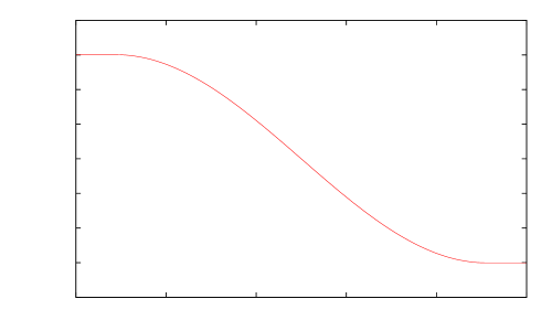
-0.8-0.6-0.4-0.200.20.40.60.800.20.40.60.81Refer to caption
Figure 9: Solution of Equation (28)
Table 11: Numerical results for optimal stopping time game (28) with a 2049×2049204920492049\times 2049 points grid, computed by AMGπ𝜋\pi with ϵ=1010italic-ϵsuperscript1010\epsilon=10^{-10}.
s𝑠{s} kmax𝑘𝑚𝑎𝑥{{k}max} rvsubscriptnormsubscript𝑟𝑣\left\|{r_{v}}\right\|_{\infty} rvL2subscriptnormsubscript𝑟𝑣subscript𝐿2\left\|{r_{v}}\right\|_{L_{2}} esubscriptnorm𝑒\left\|{e}\right\|_{\infty} eL2subscriptnorm𝑒subscript𝐿2\left\|{e}\right\|_{L_{2}} cpu time (s)
111 111 1.20e+001.20𝑒001.20e+00 7.80e017.80𝑒017.80e-01 7.75e017.75𝑒017.75e-01 2.91e012.91𝑒012.91e-01 <<1much-less-thanabsent1<<1
222 863863863 1.20e+001.20𝑒001.20e+00 2.66e022.66𝑒022.66e-02 6.02e016.02𝑒016.02e-01 3.00e013.00𝑒013.00e-01 1.58e+001.58𝑒001.58e+00
333 102510251025 1.20e+001.20𝑒001.20e+00 2.66e022.66𝑒022.66e-02 6.03e016.03𝑒016.03e-01 3.00e013.00𝑒013.00e-01 3.31e+003.31𝑒003.31e+00
\dots
100100100 102610261026 1.20e+001.20𝑒001.20e+00 2.66e022.66𝑒022.66e-02 7.10e017.10𝑒017.10e-01 2.46e012.46𝑒012.46e-01 1.81e+021.81𝑒021.81e+02
\dots
200200200 992992992 1.20e+001.20𝑒001.20e+00 2.66e022.66𝑒022.66e-02 8.16e018.16𝑒018.16e-01 1.93e011.93𝑒011.93e-01 3.75e+023.75𝑒023.75e+02
\dots
300300300 947947947 1.20e+001.20𝑒001.20e+00 2.66e022.66𝑒022.66e-02 9.16e019.16𝑒019.16e-01 1.44e011.44𝑒011.44e-01 5.72e+025.72𝑒025.72e+02
\dots
400400400 910910910 1.20e+001.20𝑒001.20e+00 2.66e022.66𝑒022.66e-02 1.00e+001.00𝑒001.00e+00 1.01e011.01𝑒011.01e-01 7.73e+027.73𝑒027.73e+02
\dots
500500500 882882882 1.20e+001.20𝑒001.20e+00 2.66e022.66𝑒022.66e-02 1.08e+001.08𝑒001.08e+00 6.59e026.59𝑒026.59e-02 9.78e+029.78𝑒029.78e+02
\dots
600600600 862862862 1.20e+001.20𝑒001.20e+00 2.66e022.66𝑒022.66e-02 1.14e+001.14𝑒001.14e+00 4.05e024.05𝑒024.05e-02 1.19e+031.19𝑒031.19e+03
\dots
700700700 849849849 1.20e+001.20𝑒001.20e+00 2.66e022.66𝑒022.66e-02 1.18e+001.18𝑒001.18e+00 2.84e022.84𝑒022.84e-02 1.41e+031.41𝑒031.41e+03
\dots
800800800 843843843 1.20e+001.20𝑒001.20e+00 2.66e022.66𝑒022.66e-02 1.20e+001.20𝑒001.20e+00 2.65e022.65𝑒022.65e-02 1.64e+031.64𝑒031.64e+03
\dots
839839839 843843843 1.20e+001.20𝑒001.20e+00 2.66e022.66𝑒022.66e-02 1.20e+001.20𝑒001.20e+00 2.66e022.66𝑒022.66e-02 1.73e+031.73𝑒031.73e+03
840840840 843843843 2.03e072.03𝑒072.03e-07 4.50e094.50𝑒094.50e-09 5.22e075.22𝑒075.22e-07 2.57e072.57𝑒072.57e-07 1.74e+031.74𝑒031.74e+03
841841841 111 1.11e161.11𝑒161.11e-16 6.57e186.57𝑒186.57e-18 1.16e071.16𝑒071.16e-07 7.40e087.40𝑒087.40e-08 1.74e+031.74𝑒031.74e+03
Table 12: Numerical results for optimal stopping time game (28) with a 2049×2049204920492049\times 2049 points grid, computed by FAMGπ𝜋\pi with c=102𝑐superscript102c=10^{-2} and ϵ=1010italic-ϵsuperscript1010\epsilon=10^{-10}.
s𝑠{s} kmax𝑘𝑚𝑎𝑥{{k}max} rvsubscriptnormsubscript𝑟𝑣\left\|{r_{v}}\right\|_{\infty} rvL2subscriptnormsubscript𝑟𝑣subscript𝐿2\left\|{r_{v}}\right\|_{L_{2}} esubscriptnorm𝑒\left\|{e}\right\|_{\infty} eL2subscriptnorm𝑒subscript𝐿2\left\|{e}\right\|_{L_{2}} cpu time (s)
points in each direction : 333, step size : 5.00e015.00𝑒015.00e-01
111 222 1.20e+001.20𝑒001.20e+00 1.20e+001.20𝑒001.20e+00 6.01e016.01𝑒016.01e-01 6.01e016.01𝑒016.01e-01 <<1much-less-thanabsent1<<1
222 222 0.00e+000.00𝑒000.00e+00 0.00e+000.00𝑒000.00e+00 5.55e175.55𝑒175.55e-17 5.55e175.55𝑒175.55e-17 <<1much-less-thanabsent1<<1
points in each direction : 555, step size : 2.50e012.50𝑒012.50e-01
111 222 1.56e011.56𝑒011.56e-01 9.02e029.02𝑒029.02e-02 1.13e011.13𝑒011.13e-01 1.03e011.03𝑒011.03e-01 <<1much-less-thanabsent1<<1
222 111 1.89e171.89𝑒171.89e-17 1.09e171.09𝑒171.09e-17 1.13e011.13𝑒011.13e-01 9.22e029.22𝑒029.22e-02 <<1much-less-thanabsent1<<1
points in each direction : 999, step size : 1.25e011.25𝑒011.25e-01
111 222 1.20e+001.20𝑒001.20e+00 4.54e014.54𝑒014.54e-01 8.74e018.74𝑒018.74e-01 3.52e013.52𝑒013.52e-01 <<1much-less-thanabsent1<<1
222 555 1.20e+001.20𝑒001.20e+00 4.54e014.54𝑒014.54e-01 1.09e+001.09𝑒001.09e+00 4.14e014.14𝑒014.14e-01 <<1much-less-thanabsent1<<1
333 555 5.55e175.55𝑒175.55e-17 2.21e172.21𝑒172.21e-17 5.74e035.74𝑒035.74e-03 4.35e034.35𝑒034.35e-03 <<1much-less-thanabsent1<<1
points in each direction : 171717, step size : 6.25e026.25𝑒026.25e-02
111 222 1.20e+001.20𝑒001.20e+00 3.10e013.10𝑒013.10e-01 1.16e+001.16𝑒001.16e+00 3.00e013.00𝑒013.00e-01 <<1much-less-thanabsent1<<1
222 101010 1.28e031.28𝑒031.28e-03 3.30e043.30𝑒043.30e-04 5.19e035.19𝑒035.19e-03 2.83e032.83𝑒032.83e-03 <<1much-less-thanabsent1<<1
333 111 0.00e+000.00𝑒000.00e+00 0.00e+000.00𝑒000.00e+00 3.36e033.36𝑒033.36e-03 2.10e032.10𝑒032.10e-03 <<1much-less-thanabsent1<<1
points in each direction : 333333, step size : 3.12e023.12𝑒023.12e-02
111 222 0.00e+000.00𝑒000.00e+00 0.00e+000.00𝑒000.00e+00 1.36e041.36𝑒041.36e-04 9.50e059.50𝑒059.50e-05 <<1much-less-thanabsent1<<1
points in each direction : 656565, step size : 1.56e021.56𝑒021.56e-02
111 222 1.20e+001.20𝑒001.20e+00 1.51e011.51𝑒011.51e-01 1.20e+001.20𝑒001.20e+00 1.51e011.51𝑒011.51e-01 <<1much-less-thanabsent1<<1
222 282828 0.00e+000.00𝑒000.00e+00 0.00e+000.00𝑒000.00e+00 7.08e057.08𝑒057.08e-05 4.94e054.94𝑒054.94e-05 <<1much-less-thanabsent1<<1
points in each direction : 129129129, step size : 7.81e037.81𝑒037.81e-03
111 222 1.20e+001.20𝑒001.20e+00 1.07e011.07𝑒011.07e-01 1.20e+001.20𝑒001.20e+00 1.07e011.07𝑒011.07e-01 <<1much-less-thanabsent1<<1
222 545454 2.78e172.78𝑒172.78e-17 3.75e183.75𝑒183.75e-18 6.66e056.66𝑒056.66e-05 3.85e053.85𝑒053.85e-05 2.00e022.00𝑒022.00e-02
points in each direction : 257257257, step size : 3.91e033.91𝑒033.91e-03
111 222 1.20e+001.20𝑒001.20e+00 7.53e027.53𝑒027.53e-02 1.20e+001.20𝑒001.20e+00 7.52e027.52𝑒027.52e-02 2.00e022.00𝑒022.00e-02
222 108108108 1.20e+001.20𝑒001.20e+00 7.53e027.53𝑒027.53e-02 1.20e+001.20𝑒001.20e+00 7.53e027.53𝑒027.53e-02 7.00e027.00𝑒027.00e-02
333 107107107 1.11e161.11𝑒161.11e-16 8.53e188.53𝑒188.53e-18 1.61e061.61𝑒061.61e-06 1.05e061.05𝑒061.05e-06 1.30e011.30𝑒011.30e-01
points in each direction : 513513513, step size : 1.95e031.95𝑒031.95e-03
111 222 1.20e+001.20𝑒001.20e+00 5.32e025.32𝑒025.32e-02 1.20e+001.20𝑒001.20e+00 5.32e025.32𝑒025.32e-02 1.30e011.30𝑒011.30e-01
222 212212212 1.11e161.11𝑒161.11e-16 9.82e189.82𝑒189.82e-18 4.53e074.53𝑒074.53e-07 3.02e073.02𝑒073.02e-07 3.00e013.00𝑒013.00e-01
points in each direction : 102510251025, step size : 9.77e049.77𝑒049.77e-04
111 222 1.20e+001.20𝑒001.20e+00 3.76e023.76𝑒023.76e-02 1.20e+001.20𝑒001.20e+00 3.76e023.76𝑒023.76e-02 3.00e013.00𝑒013.00e-01
222 422422422 1.11e161.11𝑒161.11e-16 1.15e171.15𝑒171.15e-17 1.69e071.69𝑒071.69e-07 1.18e071.18𝑒071.18e-07 9.40e019.40𝑒019.40e-01
points in each direction : 204920492049, step size : 4.88e044.88𝑒044.88e-04
111 222 2.03e072.03𝑒072.03e-07 4.50e094.50𝑒094.50e-09 5.22e075.22𝑒075.22e-07 2.57e072.57𝑒072.57e-07 9.40e019.40𝑒019.40e-01
222 111 1.11e161.11𝑒161.11e-16 8.52e188.52𝑒188.52e-18 1.16e071.16𝑒071.16e-07 7.40e087.40𝑒087.40e-08 9.50e019.50𝑒019.50e-01

7 Conclusion and perspective

In this paper, we have presented our algorithm AMGπ𝜋\pi for solving two player zero-sum stochastic games. This program combines the policy iteration algorithm with algebraic multigrid methods. Our experiences on a Isaacs equation show better results for AMGπ𝜋\pi in comparison with policy iteration combined to a direct linear solver. We observed that the most part of the computation time for the resolution of a non-linear equation (5) is used to solved the linear systems involved in the policy iteration algorithm. Hence, we noticed that the computation time of AMGπ𝜋\pi increase linearly with the size of the problem.

Furthermore, we also presented a full multi-level algorithm, called FAMGπ𝜋\pi, for solving two player zero-sum stochastic differential games. The numerical results on some stopping differential stochastic games presented here show that FAMGπ𝜋\pi improves substantially the computation time of the policy iteration algorithm for this kind of games. Indeed the computation time of FAMGπ𝜋\pi seems to be in the order of the number of discretization points whereas that of AMGπ𝜋\pi algorithm is about 160160160 to 170017001700 times greater. This is due to the large number of iterations needed by AMGπ𝜋\pi for solving this kind of games. Indeed, this number should be compared to the diameter of the graph associated to the corresponding game problem, for instance the union of all graphs of the Markov chains associated to fixed policies α𝛼{\alpha} and β𝛽{\beta}.

The FAMGπ𝜋\pi algorithm uses coarse grids discretizations of the partial differential equation and so cannot be applied directly to the dynamic programming equation of a two player zero-sum stochastic game with finite state space. One may ask if adapting the FAMGπ𝜋\pi algorithm to this kind of games is possible. Indeed, the complexity of two player zero-sum stochastic games is still unsettled, one only knows that it belongs to the complexity class of NP\capcoNP [49], and any new approach maybe useful to understand this complexity.

References

  • [1] Marianne Akian. Analyse de l’algorithme multigrille FMGH de résolution d’équations d’Hamilton-Jacobi-Bellman. In Analysis and optimization of systems (Antibes, 1990), volume 144 of Lecture Notes in Control and Inform. Sci., pages 113–122. Springer, Berlin, 1990.
  • [2] Marianne Akian. Méthodes multigrilles en contrôle stochastique. Institut National de Recherche en Informatique et en Automatique (INRIA), Rocquencourt, 1990. Thèse, Université de Paris IX (Paris-Dauphine), Paris, 1990.
  • [3] Marianne Akian, Stéphane Gaubert, and Asma Lakhoua. The max-plus finite element method for solving deterministic optimal control problems: basic properties and convergence analysis. SIAM J. Control Optim., 47(2):817–848, 2008.
  • [4] E. Altman. Flow control using the theory of zero sum Markov games. IEEE Trans. Automat. Control, 39(4):814–818, 1994.
  • [5] Randolph E. Bank and Donald J. Rose. Analysis of a multilevel iterative method for nonlinear finite element equations. Math. Comp., 39(160):453–465, 1982.
  • [6] M. Bardi, M. Falcone, and P. Soravia. Fully discrete schemes for the value function of pursuit-evasion games. In Advances in dynamic games and applications (Geneva, 1992), volume 1 of Ann. Internat. Soc. Dynam. Games, pages 89–105. Birkhäuser Boston, Boston, MA, 1994.
  • [7] Martino Bardi, Maurizio Falcone, and Pierpaolo Soravia. Numerical methods for pursuit-evasion games via viscosity solutions. In Stochastic and differential games, volume 4 of Ann. Internat. Soc. Dynam. Games, pages 105–175. Birkhäuser Boston, Boston, MA, 1999.
  • [8] G. Barles and P. E. Souganidis. Convergence of approximation schemes for fully nonlinear second order equations. Asymptotic Anal., 4(3):271–283, 1991.
  • [9] T. Başar and P. Bernhard. Hsuperscript𝐻H^{\infty}-optimal control and related minimax design problems. Systems & Control: Foundations & Applications. Birkhäuser Boston Inc., Boston, MA, second edition, 1995. A dynamic game approach.
  • [10] Richard Bellman. Dynamic programming. Princeton University Press, Princeton, N. J., 1957.
  • [11] A. Bensoussan and J.-L. Lions. Applications des inéquations variationnelles en contrôle stochastique. Dunod, Paris, 1978. Méthodes Mathématiques de l’Informatique, No. 6.
  • [12] A. Bensoussan and J.-L. Lions. Contrôle impulsionnel et inéquations quasi variationnelles, volume 11 of Méthodes Mathématiques de l’Informatique [Mathematical Methods of Information Science]. Gauthier-Villars, Paris, 1982.
  • [13] Abraham Berman and Robert J. Plemmons. Nonnegative matrices in the mathematical sciences, volume 9 of Classics in Applied Mathematics. Society for Industrial and Applied Mathematics (SIAM), Philadelphia, PA, 1994. Revised reprint of the 1979 original.
  • [14] D. P. Bertsekas. Dynamic programming. Prentice Hall Inc., Englewood Cliffs, NJ, 1987. Deterministic and stochastic models.
  • [15] Olivier Bokanowski, Stefania Maroso, and Hasnaa Zidani. Some convergence results for Howard’s algorithm. SIAM J. Numer. Anal., 47(4):3001–3026, 2009.
  • [16] J. Frédéric Bonnans and Housnaa Zidani. Consistency of generalized finite difference schemes for the stochastic HJB equation. SIAM J. Numer. Anal., 41(3):1008–1021 (electronic), 2003.
  • [17] A. Brandt, S. McCormick, and J. Ruge. Algebraic multigrid (AMG) for sparse matrix equations. In Sparsity and its applications (Loughborough, 1983), pages 257–284. Cambridge Univ. Press, Cambridge, 1985.
  • [18] Achi Brandt. Algebraic multigrid theory: the symmetric case. Appl. Math. Comput., 19(1-4):23–56, 1986. Second Copper Mountain conference on multigrid methods (Copper Mountain, Colo., 1985).
  • [19] Jean Cochet-Terrasson and Stéphane Gaubert. A policy iteration algorithm for zero-sum stochastic games with mean payoff. C. R. Math. Acad. Sci. Paris, 343(5):377–382, 2006.
  • [20] Michael G. Crandall, Hitoshi Ishii, and Pierre-Louis Lions. User’s guide to viscosity solutions of second order partial differential equations. Bull. Amer. Math. Soc. (N.S.), 27(1):1–67, 1992.
  • [21] Timothy A. Davis. Algorithm 832: Umfpack v4.3—an unsymmetric-pattern multifrontal method. ACM Trans. Math. Softw., 30:196–199, June 2004.
  • [22] E. V. Denardo and B. L. Fox. Multichain Markov renewal programs. SIAM J. Appl. Math., 16:468–487, 1968.
  • [23] Eric V. Denardo. Contraction mappings in the theory underlying dynamic programming. SIAM Rev., 9:165–177, 1967.
  • [24] Vishesh Dhingra and Stéphane Gaubert. How to solve large scale deterministic games with mean payoff by policy iteration. In valuetools ’06: Proceedings of the 1st international conference on Performance evaluation methodolgies and tools, page 12, New York, NY, USA, 2006. ACM.
  • [25] R. J. Elliott and T.K̃. Siu. A stochastic differential game for optimal investment of an insurer with regime switching. Quant. Finance, 11(3):365–380, 2011.
  • [26] Robert D. Falgout, Panayot S. Vassilevski, and Ludmil T. Zikatanov. On two-grid convergence estimates. Numer. Linear Algebra Appl., 12(5-6):471–494, 2005.
  • [27] John Fearnley. Exponential lower bounds for policy iteration. In Automata, Languages and Programming, pages 551–562, 2010.
  • [28] John Fearnley. Exponential lower bounds for policy iteration, 2010. arXiv:1003.3418v1.
  • [29] Jerzy Filar and Koos Vrieze. Competitive Markov decision processes. Springer-Verlag, New York, 1997.
  • [30] W. H. Fleming and H. M. Soner. Controlled Markov processes and viscosity solutions, volume 25 of Stochastic Modelling and Applied Probability. Springer, New York, second edition, 2006.
  • [31] W. H. Fleming and P. E. Souganidis. On the existence of value functions of two-player, zero-sum stochastic differential games. Indiana Univ. Math. J., 38(2):293–314, 1989.
  • [32] Wendell H. Fleming. Risk sensitive stochastic control and differential games. Commun. Inf. Syst., 6(3):161–177, 2006.
  • [33] Avner Friedman. Stochastic games and variational inequalities. Arch. Rational Mech. Anal., 51:321–346, 1973.
  • [34] Oliver Friedmann. An exponential lower bound for the parity game strategy improvement algorithm as we know it. In LICS, pages 145–156. IEEE Computer Society, 2009.
  • [35] A. J. Hoffman and R. M. Karp. On nonterminating stochastic games. Management Sci., 12:359–370, 1966.
  • [36] Ronald H. W. Hoppe. Multigrid methods for Hamilton-Jacobi-Bellman equations. Numer. Math., 49(2-3):239–254, 1986.
  • [37] Ronald H. W. Hoppe. Multigrid algorithms for variational inequalities. SIAM J. Numer. Anal., 24(5):1046–1065, 1987.
  • [38] Ronald A. Howard. Dynamic programming and Markov processes. The Technology Press of M.I.T., Cambridge, Mass., 1960.
  • [39] Harold J. Kushner. Probability methods for approximations in stochastic control and for elliptic equations. Academic Press [Harcourt Brace Jovanovich Publishers], New York, 1977. Mathematics in Science and Engineering, Vol. 129.
  • [40] Harold J. Kushner and Paul G. Dupuis. Numerical methods for stochastic control problems in continuous time, volume 24 of Applications of Mathematics (New York). Springer-Verlag, New York, 1992.
  • [41] P.-L. Lions and B. Mercier. Approximation numérique des équations de Hamilton-Jacobi-Bellman. RAIRO Anal. Numér., 14(4):369–393, 1980.
  • [42] Stephen F. McCormick, editor. Multigrid methods, volume 3 of Frontiers in Applied Mathematics. Society for Industrial and Applied Mathematics (SIAM), Philadelphia, PA, 1987.
  • [43] W.M. McEneaney, B.G. Fitzpatrick, and I.G. Lauko. Stochastic game approach to air operations. IEEE Trans. Aero. Elec. Systems, 40:1191–1216, 2004.
  • [44] C. Mense and R. Nabben. On algebraic multi-level methods for non-symmetric systems—comparison results. Linear Algebra Appl., 429(10):2567–2588, 2008.
  • [45] Rémi Munos and Hasnaa Zidani. Consistency of a simple multidimensional scheme for Hamilton-Jacobi-Bellman equations. C. R. Math. Acad. Sci. Paris, 340(7):499–502, 2005.
  • [46] A. Neyman and S. Sorin. Stochastic games and applications, volume 570. Springer Netherlands, 2003.
  • [47] Yvan Notay. Algebraic analysis of two-grid methods: The nonsymmetric case. Numer. Linear Algebra Appl., 17(1):73–96, 2010.
  • [48] N. Shimkin O. Ziv. Multigrid methods for policy evaluation and reinforcement learning. In Proc. IEEE International Symposium on Intelligent Control (ISIC05). IEEE, 2005.
  • [49] Anuj Puri. Theory of hybrid systems and discrete event systems. PhD thesis, Berkeley, CA, USA, 1995.
  • [50] M. L. Puterman. Markov decision processes: discrete stochastic dynamic programming. Wiley Series in Probability and Mathematical Statistics: Applied Probability and Statistics. John Wiley & Sons Inc., New York, 1994.
  • [51] Martin L. Puterman and Shelby L. Brumelle. On the convergence of policy iteration in stationary dynamic programming. Math. Oper. Res., 4(1):60–69, 1979.
  • [52] R. T. Rockafellar. Convex analysis. Princeton University Press, 1970.
  • [53] J. W. Ruge and K. Stüben. Algebraic multigrid. In Stephen F. McCormick, editor, Multigrid methods, volume 3 of Frontiers Appl. Math., pages 73–130. SIAM, Philadelphia, PA, 1987.
  • [54] L. S. Shapley. Stochastic games. In Stochastic games and applications (Stony Brook, NY, 1999), volume 570 of NATO Sci. Ser. C Math. Phys. Sci., pages 1–7. Kluwer Acad. Publ., Dordrecht, 2003. Reprint of Proc. Nat. Acad. Sci. U.S.A. 39 (1953), 1095–1100 [0061807].
  • [55] Sylvain Sorin. Classification and basic tools. In Stochastic games and applications (Stony Brook, NY, 1999), volume 570 of NATO Sci. Ser. C Math. Phys. Sci., pages 27–36. Kluwer Acad. Publ., Dordrecht, 2003.
  • [56] Andrzej Świpolhkech. Another approach to the existence of value functions of stochastic differential games. J. Math. Anal. Appl., 204(3):884–897, 1996.