Abstract

We propose an algebraic lattice supersymmetry formulation which has an exact supersymmetry on the lattice. We show how lattice version of chiral conditions can be imposed to satisfy an exact lattice supersymmetry algebra. The species doublers of chiral fermions and the corresponding bosonic counterparts can be accommodated to fit into chiral supermultiplets of lattice supersymmetry and thus lattice chiral fermion problem does not appear. We explicitly show how N=2 Wess-Zumino model in one and two dimensions can be formulated to keep exact supersymmetry for all super charges on the lattice. The momentum representation of $N=2$ lattice chiral supersymmetry algebra has lattice periodicity and thus momentum conservation should be modified to a lattice version of sine momentum conservation, which generates nonlocal interactions and leads to a loss of lattice translational invariance. It is shown that the nonlocality is mild and the translational invariance is recovered in the continuum limit. In the coordinate representation a new type of product is defined and the difference operator satisfies Leibnitz rule and an exact lattice supersymmetry is realized on this product.

PACS codes: 11.15.Ha, 11.30.Pb, 11.10.Kk.

Keywords: lattice supersymmetry, lattice field theory.

1 Introduction

Although supersymmetry has not yet been discovered in nature, it plays a crucial role in various approaches to unified theories. It is thus very natural to try to find a constructively well defined formulation of supersymmetric theories working even in the nonperturbative regime. A lattice formulation could be a good candidate. On the other hand it seems that the lattice regularization and supersymmetry does not get along with each other[1, 2, 3, 4, 5, 6]. Realization of exact lattice supersymmetry with a finite lattice spacing has been a long standing problem since the first attempt of lattice supersymmetry[7]. It has never been realized in a satisfactory way.

The lattice chiral fermion problem was also a longstanding problem but it is considered that a satisfactory understanding was reached at least for lattice QCD[8]. It is, however, not obvious that these two fundamental questions on the lattice are not related. We consider that these two problems are related in a fundamental way.

There are two major difficulties for constructing a formulation of exact supersymmetry on the lattice. Firstly the difference operator which plays the role of differential operator on the lattice does not satisfy the Leibnitz rule[7, 9]. A typical form of a lattice supersymmetry algebra would have the form: anti-commutator of two super charges is equal to a difference operator. However a supercharge operation on a product of fields should satisfy Leibnitz rule while the difference operator does not satisfy the Leibnitz rule and thus there appears an algebraic inconsistency already at the leading order of lattice constant level. Secondly there is the notorious chiral fermion problem. If we naively put massless fermions on a lattice, species doublers appear and an unbalance between the number of fermions and bosons is generated. Thus supersymmetry breaking is generated from different breaking source. This doubling of the chiral fermion problem could, however, be avoided if we adopt other fermion formulation with recently developed chiral fermion approach[8]. There appear, however, other problems due to the non-equal footing treatment of bosons and fermions[10, 11, 12, 13]. In this paper we propose a formulation to solve the above two difficulties.

As for the first difficulty it has been recognized in recent years that the reason why we cannot construct exact lattice supersymmetry models is not because it is simply difficult but it is in fact impossible if we introduce the difference operator in the lattice supersymmetry algebra and keep strictly the locality and translational invariance on the lattice[14, 15, 12]. If we give up some of the presumed characteristics such as locality, translational invariance, commutativity,… then we can find some supersymmetric lattice formulations which were claimed to be exactly supersymmetric on the lattice[16, 17, 15, 18].

We consider that there are three possibilities for exact lattice supersymmetry formulations with a lattice derivative;
(1) Keeping a local lattice derivative like difference operator but losing translational invariance on the lattice, (2) keeping finite translational invariance exact but using non-local lattice derivative like SLAC derivative[19], (3) keeping the difference operator as lattice derivative operator but introducing non-commutativity between fields, turning the algebraic structure into a Hopf algebra.

The first possibility (1) was suggested by Dondi and Nicolai[7] with a lattice version of sine momentum conservation. A possible realization of this idea was later developed in the coordinate space[16]. As a result it is equivalent to introduce a delta function of lattice momentum, leading to nonlocal interactions[20]. It has been recognized by many authors that the second possibility (2) may be the only possibility if we strictly keep the lattice translational invariance[17, 14, 15, 12]. It is, however, well known that the SLAC type derivative is highly nonlocal and may cause various problems. In particular anomaly will not be generated properly when gauge fields are turned on[21], suggesting a fundamental connection with the chiral fermion issue. An alternative analysis by a consistency condition of block spin transformation for supersymmetric lattice models led also to a statement that the only consistent lattice derivative is the SLAC derivative[22]. It is important to realize that both approaches (1) and (2) include nonlocal interactions. There was a proposal of exact supersymmetry without nonlocality but with the introduction of infinite flavors[15].

Our link approach formulation [18] of lattice supersymmetry falls into the case (3). According to the breakdown of the Leibnitz rule for the difference operator we introduced similar breaking pattern of Leibnitz rule for super charges and imposed algebraic consistency. We then claimed that the exact lattice supersymmetry is realized. It was, however, pointed out that the formulation contains an ordering ambiguity for the products of fields[23, 24]. It was later recognized that the problems caused by the ordering ambiguity can be solved by introducing a noncommutativity for fields carrying a shift. Then it was claimed that the models of link approach are exactly supersymmetric under a Hopf algebraic symmetry where the difference operator can be treated as derivative operator and the noncommutativity of fields naturally fits within the scheme of a Hopf algebra[25]. In the case of gauge theory, the problem of gauge invariance was questioned and remained to be understood.

We have so far considered the cases where the supersymmetry algebra includes a lattice differential operator. If a lattice differential operator is not included as part of the exact lattice supersymmetry formulation, then the above arguments do not apply. In fact exact lattice supersymmetry has been realized in some special case of nilpotent super charge $Q^{2}=0$ which is a part of an extended supersymmetry algebra[26, 3, 27, 28, 29, 30, 18, 31, 32, 6] in a twisted supersymmetry formulation[35]. The exactness of the nilpotent super charges of an extended supersymmetry greatly helps the lattice models to converge into supersymmetric continuum theories in lower dimensions[27], it is, however, expected that fine tunings related to other super charges may be difficult for higher dimensional models with extended supersymmetry.

In our previous paper [20], denoted in the following as paper I, we proposed a new formulation which has $N=2$ exact lattice supersymmetry in one dimension. Our formulation, however, falls into the case (1) for the first difficulty in the above classification. We introduced a lattice version of sine momentum conservation which led to nonlocal interactions and a mild loss of translational invariance. In paper I we solved the second difficulty of species doubler problem of chiral fermions by identifying the species doublers of a chiral fermion with members of its same supermultiplet of the $N=2$ supersymmetry. The species doublers of chiral fermions are physical particles and thus chiral fermion problem does not exist in this formulation. We conjectured a possibility that the approach (1) of paper I and the link approach (3) are essentially equivalent.

In this paper we extend the previously developed formulation of paper I to the $N=2$ Wess-Zumino model in two dimensions. In particular we develop a systematic treatment of chiral super fields algebraically and find chiral conditions on the lattice. Previously in paper I we found the supersymmetric action heuristically, while here we provide a formulation for deriving the action as a $Q$-exact quantity within the lattice version of chiral superfield formalism.

This paper is organized as follows: We first explain the basic concept of lattice supersymmetry in our formulation for the simplest model in section 2. In section 3 we re-derive the action of one dimensional $N=2$ supersymmetric model which was heuristically derived in paper I. Superderivatives are consistently introduced on the lattice and the basic algebraic structure of lattice chiral superfield formulation are presented for the one dimensional model. In section 4 two dimensional full treatment of the $N=2$ lattice supersymmetry algebra is given. The chiral conditions of the lattice supersymmetry algebra are derived. In section 5 the Wess-Zumino action for $D=N=2$ is derived in terms of lattice fields belonging to irreducible chiral and antichiral representations. In section 6 we introduce a new type of star product in the coordinate representation on which the difference operator satisfy the Leibnitz rule. We then express the non local action in the coordinate space in terms of the star product. The section 7 includes conclusions and discussions. In the appendix we provide an analysis of the recovery of translational invariance in the continuum limit.

2 The origin of lattice supersymmetry transformation

The simplest supersymmetry algebra in one dimension is given it terms of a single supercharge $Q$ satisfying the following relation:

$$Q^{2}=~{}i\frac{\partial}{\partial x}~{}~{},$$ (2.1)

where $i\frac{\partial}{\partial x}$ can be considered as the momentum generator. The lattice counterpart of this algebra is obtained by replacing the differential operator with a difference operator

$$Q^{2}=~{}i\partial^{(s)}~{}~{},$$ (2.2)

where we introduce the symmetric difference operator: $\partial^{(s)}$:

$$\partial^{(s)}\Phi(x)=~{}\frac{1}{a}\left\{\Phi\left(x+\frac{a}{2}\right)-\Phi\left(x-\frac{a}{2}\right)\right\}~{}~{},$$ (2.3)

where $a$ is the fundamental lattice constant.

Since $i\partial^{(s)}$ can be considered as the generator of a translation of the lattice distance $a$, it is natural to expect that the super charge $Q$ may be identified as a half lattice translation generator. It is thus very natural to introduce half lattice sites to accommodate the half lattice translation. In our previous papers we stressed that the importance of the half lattice structure in the lattice supersymmetry transformation can be well understood by the matrix formulation of the super coordinates and charges [33, 34]. Furthermore it was recognized that in the $D=N=1$ supersymmetry an alternating sign structure $(-1)^{\frac{2x}{a}},~{}(x=n\frac{a}{2},~{}n\in Z)$ on the half lattice is associated to the fermionic states. One can then write a lattice “superfield” symbolically as

$$\Phi(x)=\varphi(x)+\frac{1}{2}\sqrt{a}(-1)^{\frac{2x}{a}}\psi(x),$$ (2.4)

where we have introduced a factor $\frac{1}{2}$ and $\sqrt{a}$ for convenience. $\varphi$ and $\psi$ are, respectively, Grassman even and odd fields.

Since we identify the super charge operation as a half lattice symmetric difference operation, one is led to introduce lattice sites at integer multiples of $\frac{a}{4}$. Then the expression (2.4) actually means:

$$\Phi(x)=\left\{\begin{array}[]{lc}&\varphi(x)~{}~{}~{}~{}~{}~{}~{}~{}\textrm{for}~{}~{}~{}x=na/2,\\ &\frac{1}{2}a^{1/2}e^{\frac{2i\pi x}{a}}\psi(x)~{}~{}~{}\textrm{for}~{}~{}~{}x=(2n+1)a/4.\end{array}\right.$$ (2.5)

The supersymmetry transformations can be identified as a half lattice $\frac{a}{2}$ shift transformation of the superfield $\Phi(x)$:

$$\delta_{\alpha}\Phi(x)=\alpha a^{-1/2}e^{\frac{2i\pi x}{a}}\left[\Phi\left(x+\frac{a}{4}\right)-\Phi\left(x-\frac{a}{4}\right)\right],$$ (2.6)

where $\alpha$ is a Grassman odd super parameter accompanying an alternating sign. By separating $\Phi(x)$ into its component fields according to (2.5) we find:

$$\delta_{\alpha}\varphi(x)=\frac{i\alpha}{2}\bigg{[}\psi\left(x+\frac{a}{4}\right)+\psi\left(x-\frac{a}{4}\right)\bigg{]}\xrightarrow[a\to 0]{}i\alpha\psi(x)\,,$$ (2.7)

$$\delta_{\alpha}\psi(x)=2a^{-1}\alpha\bigg{[}\varphi\left(x+\frac{a}{4}\right)-\varphi\left(x-\frac{a}{4}\right)\bigg{]}\xrightarrow[a\to 0]{}\alpha\frac{\partial\varphi(x)}{\partial x}\,,$$ (2.8)

where $x$ is an even multiple of $a/4$ in (2.7) and an odd one in (2.8). It is rather surprising that the half lattice translation together with alternating sign structure for the lattice superfields generates a correct lattice supersymmetry transformation in the coordinate space.

The commutator of two supersymmetry transformations (2.6) leads to a translation of the lattice constant $a$ generated by the symmetric difference operator $\partial^{(s)}$ given in eq.(2.3), thus realizing the lattice supersymmetry algebra (2.2):

$$\delta_{\beta}\delta_{\alpha}\Phi(x)-\delta_{\alpha}\delta_{\beta}\Phi(x)=2\alpha\beta Q^{2}\Phi(x)=\frac{2i\alpha\beta}{a}e^{\frac{4i\pi x}{a}}\left[\Phi\left(x+\frac{a}{2}\right)-\Phi\left(x-\frac{a}{2}\right)\right].$$ (2.9)

The exponential phase factor $e^{\frac{4i\pi x}{a}}$ is $+1$ for $x=\frac{na}{2}$ and $-1$ for $x=\frac{na}{2}+\frac{a}{4}$. The same algebraic relation (2.9), but without the phase factor $e^{\frac{4i\pi x}{a}}$, works separately also for the component fields $\varphi$ and $\psi$.

In the coordinate space representation the alternating sign structure plays a crucial role in reproducing the correct lattice supersymmetry transformation and in interchanging the role of the fermion and of the boson. Let us consider the meaning of the alternating sign structure in the momentum space representation. We define the Fourier transform of the fermionic component field as

$$\psi(p)=\frac{1}{2}\sum_{x=\frac{na}{2}+\frac{a}{4}}e^{ipx}\psi(x)=-\psi\left(p\pm\frac{4\pi}{a}\right),$$ (2.10)

which has anti-periodicity with respect to a momentum shift of $\frac{4\pi}{a}$, since fermions are located on the quarter lattice sites. Let us consider now the fermion field with an accompanying alternating sign. In the momentum space representation it becomes:

$$\frac{1}{2}\sum_{x=\frac{na}{2}+\frac{a}{4}}e^{ipx}(-1)^{\frac{2x}{a}}\psi(x)=\psi\left(p+\frac{2\pi}{a}\right)=-\psi\left(p-\frac{2\pi}{a}\right).$$ (2.11)

The alternating sign of the half lattice structure corresponds in momentum space to a shift of $\pm\frac{2\pi}{a}$ in the momentum. So the fermion field with an accompanying alternating sign structure in the coordinate space may be associated to a species doubler field.

In a naive lattice formulation of chiral fermions it is known that the species doublers appear as independent fields so that the number of degrees of freedom of the fermions is increased and the matching of the degrees of freedom between bosons and fermions may be lost. However in our lattice formulation it is natural to introduce bosonic counter parts of species doublers as well, thus restoring the balance between bosons and fermions.

In fact, since the lattice spacing for each component field is $\frac{a}{2}$ ( with a relative shift of $\frac{a}{4}$ between the boson and the fermion field), but translational invariance is associated to shift of the lattice spacing $a$, for each field on the lattice there are two translational invariant configurations, namely:

$$\Phi_{1}(x)=c_{1},~{}~{}~{}~{}~{}~{}\Phi_{2}(x)=(-1)^{n}c_{2},$$ (2.12)

where $\Phi\equiv\{\varphi,\psi\}$, $x=\frac{na}{2}$ for $\Phi\equiv\varphi$ and $x=\frac{na}{2}+\frac{a}{4}$ for $\Phi\equiv\psi$.

These two configurations, being translational invariant, should have zero momentum in the continuum limit but on the lattice they have respectively momentum $0$ and $\frac{2\pi}{a}$. Fluctuations around $\Phi_{1}$ and $\Phi_{2}$ describe distinct degrees of freedom, which in the case of fermions can be described as the field and its doubler.

So, although we started from an $N=D=1$ supersymmetry we end up with enough degrees of freedom (including the doublers in the count) to accommodate an $N=2$ supersymmetry. This was accomplished in ref [20], and will be reviewed in the next section.

To summarize, the basic lattice supersymmetry structure as it emerges from the present discussion is:
The lattice supersymmetry transformation is a half lattice translation which mixes in general fields and doubler-fields, namely smooth fields on the $\frac{a}{2}$ lattice and fields with an alternating sign structure. The fermion doubling problem is solved as doublers and original fields alike are members of the same extended supersymmetry multiplet.

3 Revisit to one-dimensional $N=2$ model with lattice chiral conditions

In this section we shall give a derivation of the lattice action invariant under the $N=2$ supersymmetry in $1$ dimension. This action was found in our previous paper [20] in a more heuristic way. We shall also derive the lattice version of chiral conditions which play an important part in the derivation of the action. This formulation will be extended to the two dimensional $N=2$ Wess-Zumino model in the following sections.

There are two supercharges in the $N=2$ model, whose algebra is given as follows:

$$Q_{1}^{2}=Q_{2}^{2}=i\partial,~{}~{}~{}~{}~{}~{}~{}~{}\{Q_{1},Q_{2}\}=0,$$ (3.1)

which shows that there are two uncorrelated $N=1$ algebras of the type (2.1). One of the supersymmetry transformations, which we denote by $\delta_{1}=\alpha Q_{1}$, can be identified with (2.7) and (2.8) of the $N=1$ model:

$$Q_{1}\Phi(x)=\frac{i}{2}\bigg{[}\Psi\left(x+\frac{a}{4}\right)+\Psi\left(x-\frac{a}{4}\right)\bigg{]}~{}~{}~{}~{}~{}~{}~{}~{}x=\frac{na}{2}\,,$$

$$Q_{1}\Psi(x)=2\bigg{[}\Phi\left(x+\frac{a}{4}\right)-\Phi\left(x-\frac{a}{4}\right)\bigg{]}~{}~{}~{}~{}~{}~{}~{}~{}~{}x=\frac{na}{2}+\frac{a}{4}\,.$$ (3.2)

We assume here that $\Phi(x)$ and $\Psi(x)$ are dimensionless, so that no dependence on the lattice spacing $a$ appears at the r.h.s. of (3.2). Of course a rescaling of the fields with powers of $a$ will be needed to make contact with the fields of the continuum theory [20]. Let us introduce now the fields in momentum space defined as the Fourier transform of $\Phi(x)$ and $\Psi(x)$:

$$\Phi(p)=\frac{1}{2}\sum_{x=\frac{na}{2}}e^{ipx}\Phi(x),\,~{}~{}~{}~{}~{}~{}~{}~{}~{}~{}~{}~{}~{}~{}~{}~{}~{}~{}\,\Psi(p)=\frac{1}{2}\sum_{x=\frac{na}{2}+\frac{a}{4}}e^{ipx}\Psi(x).\,$$ (3.3)

The corresponding inverse transformations are:

$$\Phi(x)=a\int_{0}^{\frac{4\pi}{a}}\frac{dp}{2\pi}\Phi(p)e^{-ipx},\,~{}~{}~{}~{}~{}~{}~{}~{}~{}~{}~{}~{}~{}~{}~{}~{}~{}~{}\,\Psi(x)=a\int_{0}^{\frac{4\pi}{a}}\frac{dp}{2\pi}\Psi(p)e^{-ipx}.\,$$ (3.4)

From(3.3) it is clear that $\Phi(p)$ and $\Psi(p)$ satisfy the following periodicity conditions:

$$\Phi\left(p+\frac{4\pi}{a}\right)=\Phi(p),\,~{}~{}~{}~{}~{}~{}~{}~{}~{}~{}~{}~{}~{}~{}~{}~{}~{}~{}\Psi\left(p+\frac{4\pi}{a}\right)=-\Psi(p).$$ (3.5)

In momentum representation the supersymmetry transformations (3.2) read:

$$Q_{1}\Phi(p)=i\cos\frac{ap}{4}\Psi(p)\,,$$

$$Q_{1}\Psi(p)=-4i\sin\frac{ap}{4}\Phi(p)\,.$$ (3.6)

We have now to identify the second supersymmetry transformation $Q_{2}$. As discussed in [20], by comparing with the momentum representation of the continuum formulation we find that the second lattice supersymmetry transformation can be obtained by doing in (3.6) the following replacement for the fermion field:

$$\Psi(p)\longrightarrow-i\Psi\left(\frac{2\pi}{a}-p\right),$$ (3.7)

obtaining for $Q_{2}$ the following expression:

$$Q_{2}\Phi(p)=\cos\frac{ap}{4}\Psi\left(\frac{2\pi}{a}-p\right)\,,$$

$$Q_{2}\Psi\left(\frac{2\pi}{a}-p\right)=4\sin\frac{ap}{4}\Phi(p)\,.$$ (3.8)

From (3.6) and (3.8) one can check that the super charges $Q_{1}$ and $Q_{2}$ satisfy on the lattice in momentum representation the following algebra:

$$Q_{1}^{2}=Q_{2}^{2}=2\sin\frac{ap}{2},~{}~{}~{}~{}~{}~{}~{}~{}~{}~{}\{Q_{1},Q_{2}\}=0.$$ (3.9)

This is the lattice momentum version of the algebra (3.1).

We introduce now the chiral super charges

$$Q_{\pm}=\frac{1}{2}(Q_{1}\pm iQ_{2}),$$ (3.10)

which satisfy the following chiral algebra:

$$\{Q_{+},Q_{-}\}=2\sin\frac{ap}{2},~{}~{}~{}~{}~{}~{}~{}~{}~{}~{}Q_{+}^{2}=Q_{-}^{2}=0.$$ (3.11)

We want to introduce the lattice version of the superderivatives. In the superspace formalism of the continuum theory the superderivative differential operators are obtained from the corresponding supercharge operators by changing the sign of $\frac{\partial}{\partial x^{\mu}}$, namely of the momentum. In our lattice formulation where we have species doublers in the momentum representation of the half lattice structure, the correspondence between the lattice momentum and continuum momentum need to be carefully defined. We make a correspondence with the lattice momentum $p$ and continuum momentum $p_{c}$ in the following way:

$$(1)~{}\hbox{Field fluctuations around }~{}p=0;~{}~{}~{}p=p_{c},$$

$$(2)~{}\hbox{Species doublers fluctuations around}~{}p=\frac{2\pi}{a};~{}~{}~{}p=\frac{2\pi}{a}-p_{c}.$$ (3.12)

In the lattice momentum region (1), the sign change of momentum $p_{c}\rightarrow-p_{c}$ corresponds to the following change of the coefficients in the supersymmetry transformation:

$$\cos\frac{ap}{4}~{}\rightarrow~{}\cos\frac{ap}{4},~{}~{}~{}\sin\frac{ap}{4}~{}\rightarrow~{}-\sin\frac{ap}{4},$$ (3.13)

while in the region (2) the sign change of momentum $p_{c}\rightarrow-p_{c}$ corresponds to

$$\cos\frac{ap}{4}~{}=~{}\cos\frac{a}{4}\left(\frac{2\pi}{a}-p_{c}\right)~{} \rightarrow ~{}\cos\frac{a}{4}\left(\frac{2\pi}{a}+p_{c}\right)~{}=~{}-\cos\frac{ap}{4}$$

$$\sin\frac{ap}{4}~{}=~{}\sin\frac{a}{4}\left(\frac{2\pi}{a}-p_{c}\right)~{} \rightarrow ~{}\sin\frac{a}{4}\left(\frac{2\pi}{a}+p_{c}\right)~{}=~{}\sin\frac{ap}{4}.$$ (3.14)

Thus the sign changes of $\cos\frac{ap}{4}$ and $\sin\frac{ap}{4}$ are opposite in the region (1) and (2). To connect smoothly eq. (3.13) to eq. (3.14) one can multiply the right hand sides by a factor $\cos\frac{ap}{2}$, which just provides a $-1$ factor at $p=\frac{2\pi}{a}$. Hence to obtain the lattice superderivative from the supersymmetry transformation we simply do the following replacements:

$$\cos\frac{ap}{4}~{}\rightarrow~{}\cos\frac{ap}{2}\cos\frac{ap}{4},~{}~{}~{}\sin\frac{ap}{4}~{}\rightarrow~{}-\cos\frac{ap}{2}\sin\frac{ap}{4}.$$ (3.15)

The explicit form of the $N=2$ superderivative in one dimension acting on the component fields is:

$$D_{1}\Phi(p)=i\cos\frac{ap}{2}\cos\frac{ap}{4}\Psi(p)\,,~{}~{}~{}D_{2}\Phi(p)=\cos\frac{ap}{2}\cos\frac{ap}{4}\Psi\left(\frac{2\pi}{a}-p\right)\,,$$

$$D_{1}\Psi(p)=4i\cos\frac{ap}{2}\sin\frac{ap}{4}\Phi(p)\,,~{}~{}~{}D_{2}\Psi\left(p\right)=4\cos\frac{ap}{2}\cos\frac{ap}{4}\Phi\left(\frac{2\pi}{a}-p\right)\,$$ (3.16)

which satisfy the following algebra:

$$D_{1}^{2}~{}=~{}D_{2}^{2}~{} = ~{}-2\cos^{2}\frac{ap}{2}\sin\frac{ap}{2},~{}~{}~{}~{}~{}\{D_{1},D_{2}\}~{}=~{}0,$$ (3.17)

$$\{Q_{i},D_{j}\}~{} = ~{}0~{}~{}~{}(i,j=1,2).$$ (3.18)

Notice that the factor $\cos\frac{ap}{2}$, while essential to establish the anticommuting nature of $Q_{i}$ and $D_{i}$, does not change the algebraic structure in the continuum limit.

In analogy to chiral supercharges chiral superderivatives are defined as:

$$D_{\pm}~{}=~{}\frac{1}{2}(D_{1}~{}\pm~{}iD_{2}),$$ (3.19)

which satisfy the chiral algebra together with (3.11),

$$D_{+}^{2}~{}=~{}D_{-}^{2} = 0,~{}~{}~{}\{D_{+},D_{-}\}~{}=~{}-2\cos^{2}\frac{ap}{2}\sin\frac{ap}{2}$$

$$\{Q_{\pm},D_{\pm}\} = \{Q_{\pm},D_{\mp}\}~{}=~{}0.$$ (3.20)

Chiral conditions on the lattice can now be imposed:

$$D_{-}\Phi(p) = i\cos\frac{ap}{2}\cos\frac{ap}{4}\frac{1}{2}\left\{\Psi(p)~{}-~{}\Psi\left(\frac{2\pi}{a}-p\right)\right\}~{}=~{}0,$$ (3.21)

$$D_{-}\Psi(p) = i\sin ap~{}~{}\frac{1}{2}\left\{\frac{\Phi(p)}{\cos\frac{ap}{4}}-\frac{\Phi\left(\frac{2\pi}{a}-p\right)}{\sin\frac{ap}{4}}\right\}~{}=~{}0.$$ (3.22)

The first chiral condition (3.21) simply states that

$$\Psi(p)=\Psi(\frac{2\pi}{a}-p)$$ (3.23)

namely that the doublers degree of freedom is the same as the original fermion field. The second condition (3.22) has a similar interpretation in terms of the rescaled field

$$\underline{\Phi}(p)\equiv\frac{\Phi(p)}{\cos\frac{ap}{4}},$$ (3.24)

namely:

$$\underline{\Phi}(p)~{}=~{}\underline{\Phi}\left(\frac{2\pi}{a}-p\right).$$ (3.25)

The antichiral conditions are obtained by imposing $D_{+}\Phi(p)=D_{+}\Psi(p)=0$ and lead to similar conditions, but with a minus sign at the r.h.s. of (3.23) and of (3.25). So if we decompose $\underline{\Phi}$ and $\Psi$ as:

$$\underline{\Phi}(p)=\underline{\Phi}^{(c)}(p)+\underline{\Phi}^{(a)}(p),~{}~{}~{}~{}~{}~{}\Psi(p)=\Psi^{(c)}(p)+\Psi^{(a)}(p)$$ (3.26)

with

$$2\underline{\Phi}^{(c)}(p) = \underline{\Phi}(p)+\underline{\Phi}\left(\frac{2\pi}{a}-p\right),~{}~{}~{}~{}~{}2\underline{\Phi}^{(a)}(p)=\underline{\Phi}(p)-\underline{\Phi}\left(\frac{2\pi}{a}-p\right),$$

$$2\Psi^{(c)}(p) = \Psi(p)+\Psi\left(\frac{2\pi}{a}-p\right),~{}~{}~{}~{}~{}2\Psi^{(a)}(p)=\Psi(p)-\Psi\left(\frac{2\pi}{a}-p\right).$$ (3.27)

$\underline{\Phi}^{(c)}$ and $\Psi^{(c)}$ are the components of a chiral superfield on the lattice, whereas $\underline{\Phi}^{(a)}$ and $\Psi^{(a)}$ are the components of an antichiral superfield. So eq. (3.26) gives the decomposition of $\underline{\Phi}$ and $\Psi$ into its irreducible chiral and antichiral representations of the supersymmetry algebra.

The supersymmetry transformations of the chiral and anti-chiral fields are given in Table 1, which also shows clearly that each of them form an irreducible representation of the algebra. Notice that due to the definition (3.24) both $\underline{\Phi}(p)$ and $\Psi(p)$ change sign when $p$ is shifted of $\frac{4\pi}{a}$. In coordinate space this means that they are both located on odd integer multiples of $\frac{a}{4}$.

$\begin{array}[]{|l|c|c|}\hline\cr&\displaystyle Q_{+}&\displaystyle Q_{-}\\ \hline\cr\hline\cr\underline{\Phi}^{(c)}(p)&i\Psi^{(c)}(p)&0\\ \Psi^{(c)}(p)&0&-2i\sin\frac{ap}{2}\underline{\Phi}^{(c)}(p)\\ \underline{\Phi}^{(a)}(p)&0&i\Psi^{(a)}(p)\\ \Psi^{(a)}(p)&-2i\sin\frac{ap}{2}\underline{\Phi}^{(a)}(p)&0\\ \hline\cr\end{array}$

Table 1: Chiral and anti-chiral $N=2$ supersymmetry transformation

However one can see from Table 1 that the supersymmetry transformations are also consistent with $\underline{\Phi}^{(c)}(p)$ and $\Psi^{(c)}(p)$ being both periodic in $p$ ( same for $\underline{\Phi}^{(a)}(p)$ and $\Psi^{(a)}(p)$). This can be achieved by simply shifting the origin of the coordinate space by $\frac{a}{4}$, in particular we could have defined from the very beginning the fermionic field $\Psi(x)$ on integer multiples of $\frac{a}{2}$ and the bosonic field $\Phi(x)$ on the half integer ones.

However a shift of the origin is not without consequences with respect to the symmetry under $p\to\frac{2\pi}{a}-p$. In fact a shift of $\frac{a}{4}$ in $x$ amounts to a multiplication by $e^{i\frac{ap}{4}}$ in momentum space, and this is not invariant under $p\to\frac{2\pi}{a}-p$.

If we assume, consistently with the definition of chiral and antichiral superderivatives, that chiral and antichiral superfields are hermitian conjugate, then one can prove that antiperiodicity in the momentum implies that chiral and antichiral fields have opposite symmetry with respect to $p\to\frac{2\pi}{a}-p$ (as in the example above), whereas periodicity in the momentum requires that chiral and antichiral fields have the same symmetry with respect to $p\to\frac{2\pi}{a}-p$ (both symmetric or both antisymmetric).

So both choices are ultimately allowed and this arbitrariness will eventually come useful in building the action, particularly in the more complex two dimensional case. We want now to re-derive the action for an $n$-point interaction, action that in ref. [20] was essentially postulated.

In momentum representation the $n$-point interaction term will be expressed as an integral over the $n$ momenta of the fields. Each integration will be over a period of $\frac{4\pi}{a}$, so a condition to be required for the action density is to be periodic of period $\frac{4\pi}{a}$ in each momentum. Moreover consider, for each momentum $p_{i}$, the reflection symmetry with respect to the point $\frac{2\pi}{a}$, namely the symmetry $p_{i}\to\frac{2\pi}{a}-p_{i}$, is required. It is easy to see that, being the integration interval $(-\frac{\pi}{a},\frac{3\pi}{a})$ symmetric with respect to the point $\frac{2\pi}{a}$, the odd (antisymmetric) part of the action density vanishes identically.

A supersymmetric invariant action can be written using the $Q$-exact expression

$$\mathcal{L}(p_{1},p_{2},\cdots,p_{n})=-\frac{1}{n}\delta\left(\sin\frac{ap_{1}}{2}+\cdots+\sin\frac{ap_{n}}{2}\right)Q_{+}Q_{-}\left[\Phi(p_{1})\Phi(p_{2})\cdots\Phi(p_{n})\right]$$ (3.28)

The right hand side in (3.28) can be calculated using the explicit form of supersymmetry transformations, and gives:

$$\mathcal{L}(p_{1},p_{2},\cdots,p_{n})=\delta\left(\sin\frac{ap_{1}}{2}+\cdots+\sin\frac{ap_{n}}{2}\right)$$ (3.29)

$$\{2\sin^{2}\frac{ap_{1}}{4}~{}\Phi(p_{1})\Phi(p_{2})\cdots\Phi(p_{n})+\frac{n-1}{4}\sin\frac{a(p_{1}-p_{2})}{4}\Psi(p_{1})\Psi(p_{2})\Phi(p_{3})\cdots\Phi(p_{n})\}$$

which coincides with the expression given in ref. [20] . The invariance of $\mathcal{L}(p_{1},p_{2},\cdots,p_{n})$ under supersymmetry transformation follows immediately from the supersymmetry algebra (3.11) and the sine momentum conservation. According to our original choice $\Phi(p)$ is periodic in $p$ with period $\frac{4\pi}{a}$ and so this property is extended to $\mathcal{L}(p_{1},p_{2},\cdots,p_{n})$. So the invariant action can be written as:

$$S_{n}=\int_{-\frac{\pi}{a}}^{\frac{3\pi}{a}}dp_{1}dp_{2}\cdots dp_{n}\left(\prod_{j=1}^{n}\cos\frac{ap_{j}}{2}\right)\mathcal{L}(p_{1},p_{2},\cdots,p_{n})$$ (3.30)

where the product of cosines has been introduced, as in reference [20], to compensate singularities of the integration volume at $p_{i}=\pm\frac{\pi}{a}$ arising from the $\delta$-function. Notice that, according to what mentioned earlier about the symmetry under $p_{i}\to\frac{2\pi}{a}-p_{i}$, only the symmetric part of $\Phi(p_{i})$, namely $\frac{1}{2}(\Phi(p_{i})+\Phi(\frac{2\pi}{a}-p_{i}))$ contributes to the action. However $\Phi$ is not the normalized field $\underline{\Phi}$, and its symmetric part is not a pure chiral field but contains a mixture of chiral and anti-chiral components. This is different from what happens in the $N=D=2$ case, where the action will be constructed using chiral and anti-chiral fields.

4 $N=2$ $D=2$ chiral superfields on the lattice

In this section we shall generalize the previous approach to a two dimensional $N=2$ supersymmetry algebra. In extending the structure of the one dimensional lattice supersymmetry transformation into two dimensions, it is important to realize how one dimensional supersymmetry algebra is included in the two dimensional algebra. $N=2$ extended supersymmetry algebra in two dimensions is given by

$$\{Q_{\alpha i},Q_{\beta j}\}~{}=~{}2\delta_{ij}(\gamma^{\mu})_{\alpha\beta}i\partial_{\mu},$$ (4.1)

where we may use an explicit representation of Pauli matrices for $\gamma^{\mu}=\{\sigma^{3},\sigma^{1}\}$. By going to the light cone directions this two dimensional $N=2$ algebra can be decomposed into the direct sum of two one dimensional $N=2$ algebra :

$$\{Q_{\pm}^{(i)},Q_{\pm}^{(j)}\}~{}=~{}2\delta^{ij}i\partial_{\pm},~{}~{}~{}~{}~{}~{}\{\hbox{others}\}=0,$$ (4.2)

where

$$Q_{\pm}^{(j)}~{}=~{}\frac{Q_{1j}\pm iQ_{2j}}{\sqrt{2}},~{}~{}~{}~{}~{}~{}\partial_{\pm}=\partial_{1}\pm i\partial_{2},$$ (4.3)

where in terms of euclidean light cone coordinates

$$x_{\pm}=x_{1}\pm ix_{2},~{}~{}~{}~{}~{}~{}\partial_{\pm}=\frac{\partial}{\partial x_{\pm}}.$$ (4.4)

We can also equivalently express it in a chiral form:

$$\{Q_{+}^{(+)},Q_{+}^{(-)}\}~{}=~{}i\partial_{+},~{}~{}~{}\{Q_{-}^{(+)},Q_{-}^{(-)}\}~{}=~{}i\partial_{-},~{}~{}~{}\{\hbox{others}\}=0,$$ (4.5)

where

$$Q_{\pm}^{(+)}=\frac{Q_{\pm}^{(1)}+iQ_{\pm}^{(2)}}{2},~{}~{}~{}Q_{\pm}^{(-)}=\frac{Q_{\pm}^{(1)}-iQ_{\pm}^{(2)}}{2}.$$ (4.6)

Finally we can introduce the Dirac-Kähler twisting procedure by defining twisted super charges[35, 18]:

$$Q_{\alpha i}=(Q{\bf 1}+Q_{\mu}\gamma^{\mu}+\gamma^{2}\gamma^{1}\tilde{Q})_{\alpha i},$$ (4.7)

that satisfy the following twisted supersymmetry algebra:

$$\{Q,Q_{\mu}\}=i\partial_{\mu},~{}~{}~{}~{}~{}~{}\{\tilde{Q},Q_{\mu}\}=\epsilon_{\mu\nu}i\partial_{\nu}.$$ (4.8)

The twisted super charges are related to the chiral super charges by:

$$Q_{+}^{(+)}=\frac{Q_{1}+iQ_{2}}{\sqrt{2}}, ~{}~{}Q_{-}^{(-)}=\frac{Q_{1}-iQ_{2}}{\sqrt{2}},$$

$$Q_{+}^{(-)}=\frac{Q+i\tilde{Q}}{\sqrt{2}}, ~{}~{}Q_{-}^{(+)}=\frac{Q-i\tilde{Q}}{\sqrt{2}}.$$ (4.9)

As we can see from (4.2), we basically introduce the one dimensional lattice supersymmetry structure in each light cone direction to construct the $D=N=2$ lattice supersymmetry formulation. We shall show later that the chiral version of algebra (4.5) plays an important role in constructing chiral and anti-chiral irreducible representations of the algebra on the lattice.

In analogy with the one dimensional case we introduce in each light cone direction the one dimensional half lattice structure. In order to introduce a lattice structure on the light cone coordinates we need$x_{\pm}$ to be real quantities. Therefore we have to go from Euclidean to Minkowsky metric, namely, replace in (4.4) $ix_{2}$ with $x_{2}$. So in the following we shall refer to the light cone coordinates $x_{\pm}$ as the ones in Minkowsky space, namely $x_{\pm}=x_{1}\pm x_{2}$.

The half lattice sites on the light cone coordinate can then be represented by

$$\vec{x}_{\pm}=(n\frac{a}{2},~{}m\frac{a}{2}),~{}~{}~{}~{}~{}~{}n,m\in{\bf Z},$$ (4.10)

where $a$ is the lattice spacing associated to an elementary translation. As in the one dimensional case shifts of $\frac{a}{2}$ will be associated to supersymmetry transformations. The lattice is illustrated in Fig. 1. It is composed by the union of four lattices each with spacing $a$ in the light cone directions. These lattices are represented in the figure by different types of dots. The lattice with black dots on the sites represents points of the form $(x_{+},x_{-})=(n^{\prime}a,m^{\prime}a)$ with $n^{\prime}=\frac{n}{2}$ and $m^{\prime}=\frac{m}{2}$ both integers. In the other lattices the integers $(n,m)$ are as follows: (odd,odd) on the sites with white dots, (odd, even) on the sites with crosses and (even,odd) on the sites with circular crosses. For instance the lattice with black dots on the sites represent points with $m$ and $n$ in (4.10) both even, namely points of the form $(x_{1},x_{2})=(n^{\prime}a,m^{\prime}a)$ with $n^{\prime},m^{\prime}\in{\bf Z}$. Similarly the lattice with white dots has the structure $(x_{1},x_{2})=(n^{\prime}a+\frac{a}{2},m^{\prime}a+\frac{a}{2})$, and so on. Points belonging to the same lattice can be reached from each other by shifts which are integer multiples of $a$ in each light cone direction, namely they can be reached by translations. Points belonging to different lattices, for instance a black dot site and a white dot site, cannot be reached from each other by translations as shifts which are odd multiples of $\frac{a}{2}$ are involved.

As a result of the existence in our lattice of four distinct translational invariant sublattices, there are four distinct translational invariant field configurations, namely:

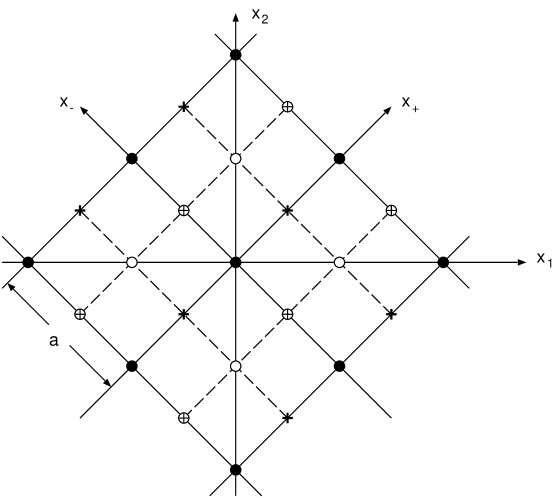
Figure 1: Light cone coordinate versus Cartesian coordinate

$$\Phi_{1}(\vec{x})=c_{1},~{}~{}~{}~{}~{}~{}\Phi_{2}(\vec{x})=(-1)^{n}c_{2},~{}~{}~{}~{}~{}~{}\Phi_{3}(\vec{x})=(-1)^{m}c_{3},~{}~{}~{}~{}~{}~{}\Phi_{4}(\vec{x})=(-1)^{n+m}c_{4},$$ (4.11)

where the $c_{i}$ s are constants and $n$ and $m$ refer to (4.10). So for instance $\Phi_{1}(\vec{x})$ is $c_{1}$ on all sites, but $~{}\Phi_{2}(\vec{x})$ is $c_{2}$ on the sites with black dots and circular crosses and $-c_{2}$ on the others, and so on.

Considering that physical fields are small fluctuations around a constant, i.e. translational invariant, configuration, it is clear from the previous discussion that a lattice field corresponds now to four physical degrees of freedom. These can be naturally identified with species doubler states, and this phase reminds us of the staggered phase of staggered fermion[37].

The algebra (4.2) has $4$ supercharges, hence an $N=2$ superfield depends on $4$ odd Grassmann variables $\theta^{(i)}_{\pm}$ and its expansion contains $16$ component fields. As in the one dimensional case we shall proceed by considering first the $N=1$ case, and by giving a realization of the $N=1$ superalgebra on a two dimensional lattice with spacing $\frac{a}{2}$. Since an $N=1$ superfield in $D=2$ contains $4$ component fields ($2$ bosonic and $2$ fermionic), the lattice realization of the $N=1$ superalgebra is done in terms of four fields on the lattice. However, because of the $\frac{a}{2}$ spacing, each field on the lattice comes together with three “doublers” and eventually corresponds to four degrees of freedom in the continuum for a total of $16$ degrees of freedom. We will then show that these $16$ degrees of freedom provide a representation on the lattice of the $N=2$ superalgebra, with the doublers of a field being different members of the same supermultiplet.

4.1 $N=1$,$D=2$ superalgebra on the lattice

Consider the $N=1$ subalgebra of (4.2) obtained by setting, for instance, $i=j=1$. The superfield expansion in this case is given by:

$$\Phi(x_{+},x_{-},\theta_{+}^{(1)},\theta_{-}^{(1)})=\varphi(x_{+},x_{-})+i\theta_{+}^{(1)}\psi_{1}(x_{+},x_{-})+i\theta_{-}^{(1)}\psi_{2}(x_{+},x_{-})+i\theta_{-}^{(1)}\theta_{+}^{(1)}F(x_{+},x_{-}),$$ (4.12)

and the supersymmetry transformations are:

$$\delta^{(1)}_{+}\varphi=i\alpha_{+}\psi_{1},~{}~{}~{}~{}~{}\delta^{(1)}_{+}\psi_{1}=\alpha_{+}\frac{\partial\varphi}{\partial x_{+}},$$

$$\delta^{(1)}_{+}\psi_{2}=\alpha_{+}F,~{}~{}~{}~{}~{}\delta^{(1)}_{+}F=i\alpha_{+}\frac{\partial\psi_{2}}{\partial x_{+}}.$$ (4.13)

and

$$\delta^{(1)}_{-}\varphi=i\alpha_{-}\psi_{2},~{}~{}~{}~{}~{}\delta^{(1)}_{-}\psi_{2}=\alpha_{-}\frac{\partial\varphi}{\partial x_{-}},$$

$$\delta^{(1)}_{-}\psi_{1}=-\alpha_{-}F,~{}~{}~{}~{}~{}\delta^{(1)}_{-}F=-i\alpha_{-}\frac{\partial\psi_{1}}{\partial x_{-}}.$$ (4.14)

In order to put this system on a lattice we proceed in the same way as in the $N=1$,$D=1$, treating the two light cone variables independently. The lattice spacing is $\frac{a}{2}$ for both $x_{+}$ and $x_{-}$, but in order to introduce a half lattice difference operator we need to introduce sites on the multiples of $\frac{a}{4}$ as well. A rather direct generalization of (2.5) is:

$$\Xi(x_{+},x_{-})=\left\{\begin{array}[]{lc}\Phi(x_{+},x_{-}){}{}{}{}{}{}{}{}&\textrm{for}~{}~{}~{}x_{+},x_{-}=na/2,\\ \frac{1}{2}e^{\frac{2i\pi x_{+}}{a}}\Psi_{1}(x_{+},x_{-}){}{}{}&\textrm{for}~{}~{}~{}x_{+}=(2n+1)a/4~{}~{}\textrm{and}~{}~{}x_{-}=ma/2,\\ \frac{1}{2}e^{\frac{2i\pi x_{-}}{a}}\Psi_{2}(x_{+},x_{-}){}{}{}&\textrm{for}~{}~{}~{}x_{-}=(2n+1)a/4~{}~{}\textrm{and}~{}~{}x_{+}=ma/2,\\ -\frac{i}{4}e^{\frac{2i\pi(x_{+}+x_{-})}{a}}F(x_{+},x_{-}){}{}{}{}{}{}{}{}&\textrm{for}~{}~{}~{}x_{+},x_{-}=(2n+1)a/4.\end{array}\right.$$ (4.15)

See Fig. 2 how the component fields are located in the $a/4$ lattice sites.

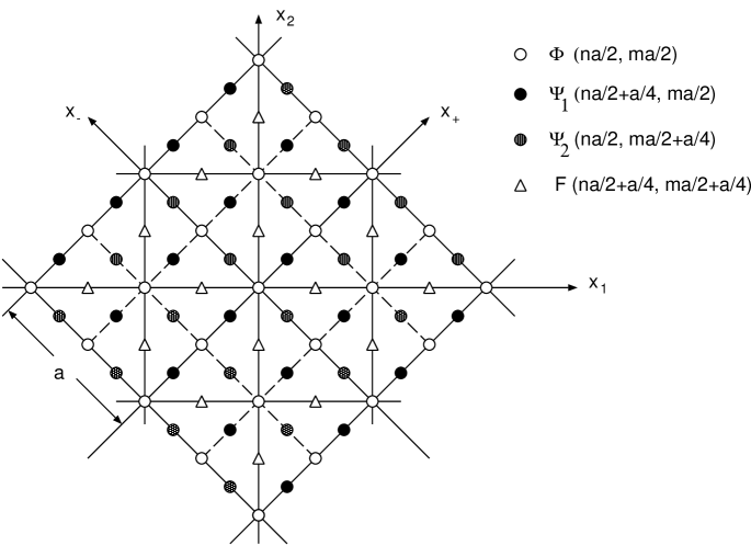
Figure 2: Fields defined on $a/4$ lattice sites.

As in the one dimensional case the supersymmetry transformation in one of the light cone directions can be defined as a finite difference over a half lattice spacing $\frac{a}{2}$ of the superfield $\Xi(x_{+},x_{-})$ :

$$\delta^{(1)}_{+}\Xi(x_{+},x_{-})=\alpha_{+}e^{\frac{2i\pi x_{+}}{a}}\left[\Xi(x_{+}+\frac{a}{4},x_{-})-\Xi(x_{+}-\frac{a}{4},x_{-})\right],$$ (4.16)

where $\alpha_{+}$ is the Grassmann odd parameters of the supersymmetry transformation. The commutator of two $\delta^{(1)}_{+}$ transformations with parameters $\alpha_{+}$,$\beta_{+}$ gives a translation:

$$\left(\delta^{(1)}_{+\alpha}\delta^{(1)}_{+\beta}-\delta^{(1)}_{+\beta}\delta^{(1)}_{+\alpha}\right)\Xi(x_{+},x_{-})=2i\beta\alpha e^{\frac{4i\pi x_{+}}{a}}\left[\Xi(x_{+}+\frac{a}{2},x_{-})-\Xi(x_{+}-\frac{a}{2},x_{-})\right].$$ (4.17)

In terms of the component fields the supersymmetry transformation (4.16) reads:

$$\delta^{(1)}_{+}\Phi(x_{+},x_{-})= \frac{i\alpha_{+}}{2}\left[\Psi_{1}(x_{+}+\frac{a}{4},x_{-})+\Psi_{1}(x_{+}-\frac{a}{4},x_{-})\right],$$

$$\delta^{(1)}_{+}\Psi_{1}(x_{+},x_{-})= 2\alpha_{+}\left[\Phi(x_{+}+\frac{a}{4},x_{-})-\Phi(x_{+}-\frac{a}{4},x_{-})\right],$$

$$\delta^{(1)}_{+}\Psi_{2}(x_{+},x_{-})= \frac{\alpha}{2}\left[F(x_{+}+\frac{a}{4},x_{-})+F(x_{+}-\frac{a}{4},x_{-})\right],$$

$$\delta^{(1)}_{+}F(x_{+},x_{-})= 2i\alpha_{+}\left[\Psi_{2}(x_{+}+\frac{a}{4},x_{-})-\Psi_{2}(x_{+}-\frac{a}{4},x_{-})\right],$$ (4.18)

and the commutator (4.17) is, for any of the component fields:

$$\left(\delta^{(1)}_{+\alpha}\delta^{(1)}_{+\beta}-\delta^{(1)}_{+\beta}\delta^{(1)}_{+\alpha}\right)\Phi_{A}(x_{+},x_{-})=2i\alpha\beta\left[\Phi_{A}(x_{+}+\frac{a}{2},x_{-})-\Phi_{A}(x_{+}-\frac{a}{2},x_{-})\right],$$ (4.19)

where $\Phi_{A}\equiv\{\Phi,\Psi_{1},\Psi_{2},F\}$.

The supersymmetry transformation along the other light cone direction $x_{-}$ requires some care. Simply exchanging $x_{+}$ and $x_{-}$ in (4.16) would amount to exchanging $\Psi_{1}$ and $\Psi_{2}$, while we know from the continuum transformations (4.13, 4.14) that $\delta^{(1)}_{-}$ is obtained from $\delta^{(1)}_{+}$ by the exchanges $x_{+}\leftrightarrow x_{-}$, $\psi_{1}\leftrightarrow\psi_{2}$ and $F\leftrightarrow-F$. The correct prescription for $\delta^{(1)}_{-}$ is to exchange in (4.16) $x_{+}$ and $x_{-}$ and replace at the same time the superfield $\Xi(x_{+},x_{-})$ with its hermitian conjugate $\Xi^{\dagger}(x_{+},x_{-})$. With all component fields hermitian $\Xi^{\dagger}$ is the same as $\Xi$ but for a change of sign of $\Psi_{1}$,$\Psi_{2}$ and $F$. An immaterial change of sign of the supersymmetry parameter $\alpha_{-}$ compensates for the sign change of $\Psi_{1}$ and $\Psi_{2}$ so that taking the hermitian conjugate of $\Xi$ amounts to changing the sign of $F$.

So the supersymmetry transformation $\delta^{(1)}_{-}$ can be written:

$$\delta^{(1)}_{-}\Xi^{\dagger}(x_{+},x_{-})=-\alpha_{-}e^{\frac{2i\pi x_{-}}{a}}\left[\Xi^{\dagger}(x_{+},x_{-}+\frac{a}{4})-\Xi^{\dagger}(x_{+},x_{-}-\frac{a}{4})\right],$$ (4.20)

or, taking the hermitian conjugate of both sides:

$$\delta^{(1)}_{-}\Xi(x_{+},x_{-})=-\left[\Xi(x_{+},x_{-}+\frac{a}{4})-\Xi(x_{+},x_{-}-\frac{a}{4})\right]\alpha_{-}e^{-\frac{2i\pi x_{-}}{a}}.$$ (4.21)

A direct check, using (4.21), shows that the commutator of two supersymmetry transformations $\delta^{(1)}_{-}$ produces a translation, exactly as in the case of $\delta^{(1)}_{+}$ (4.17). The commutator of a $\delta^{(1)}_{-}$ and a $\delta^{(1)}_{+}$ transformation vanishes. In terms of the component fields the supersymmetry transformation is, as expected, the same as (4.18) with the two light cone directions exchanged and an extra sign change of $F$:

$$\delta^{(1)}_{-}\Phi(x_{+},x_{-})= \frac{i\alpha_{-}}{2}\left[\Psi_{2}(x_{+},x_{-}+\frac{a}{4})+\Psi_{2}(x_{+},x_{-}-\frac{a}{4})\right],$$

$$\delta^{(1)}_{-}\Psi_{2}(x_{+},x_{-})= 2\alpha_{-}\left[\Phi(x_{+},x_{-}+\frac{a}{4})-\Phi(x_{+},x_{-}-\frac{a}{4})\right],$$

$$\delta^{(1)}_{-}\Psi_{1}(x_{+},x_{-})= -\frac{\alpha_{-}}{2}\left[F(x_{+},x_{-}+\frac{a}{4})+F(x_{+},x_{-}-\frac{a}{4})\right],$$

$$\delta^{(1)}_{-}F(x_{+},x_{-})= -2i\alpha_{-}\left[\Psi_{1}(x_{+},x_{-}+\frac{a}{4})-\Psi_{1}(x_{+},x_{-}-\frac{a}{4})\right].$$ (4.22)

In conclusion, the supersymmetry transformations (4.18) and (4.22) provide a representation on the lattice of the $N=1$, $D=2$ susy algebra and reproduce the continuum transformations (4.13) and (4.14) in the continuum limit. However a simple counting of the degrees of freedom shows that each field on the lattice corresponds to $4$ degrees of freedom in the continuum. This is due to the lattice spacing being $\frac{a}{2}$ while translational invariance is still associated to shifts of the original lattice spacing $a$. This means that for each fields on the lattice there are four translational invariant configurations (namely zero momentum configurations in the continuum). In fact a translational invariant configuration can be either constant or constant in absolute value but with alternating sign along each light cone direction. So to each value of the momentum in the continuum along a light cone direction will correspond on the lattice two distinct values of the momentum defined on the lattice with spacing $\frac{a}{2}$. This can be better seen in the momentum representation for the component fields defined by the Fourier transform and its inverse:

$$\Phi_{A}(p_{+},p_{-})= \frac{1}{4}\sum_{x_{+},x_{-}}e^{i(p_{+}x_{+}+p_{-}x_{-})}\Phi_{A}(x_{+},x_{-}),$$

$$\Phi_{A}(x_{+},x_{-})= \frac{a^{2}}{4\pi^{2}}\int_{0}^{\frac{4\pi}{a}}dp_{+}dp_{-}\Phi_{A}(p_{+},p_{-})e^{-i(p_{+}x_{+}+p_{-}x_{-})},$$ (4.23)

where as before $\Phi_{A}\equiv\{\Phi,\Psi_{1},\Psi_{2},F\}$ and where in the sums $x_{+}$ and $x_{-}$ are defined according to eq. (4.15). In momentum representation the component fields are periodic (resp. antiperiodic) with period $\frac{4\pi}{a}$ whenever in coordinate representation are defined on integer multiples of $\frac{a}{2}$ (resp. half-integer multiples). So we have:

$$\Phi(p_{+},p_{-})= \Phi(p_{+}+\frac{4\pi}{a},p_{-})=\Phi(p_{+},p_{-}+\frac{4\pi}{a}),$$

$$\Psi_{1}(p_{+},p_{-})= -\Psi_{1}(p_{+}+\frac{4\pi}{a},p_{-})=\Psi_{1}(p_{+},p_{-}+\frac{4\pi}{a}),$$

$$\Psi_{2}(p_{+},p_{-})= \Psi_{2}(p_{+}+\frac{4\pi}{a},p_{-})=-\Psi_{2}(p_{+},p_{-}+\frac{4\pi}{a}),$$

$$F(p_{+},p_{-})= -F(p_{+}+\frac{4\pi}{a},p_{-})=-F(p_{+},p_{-}+\frac{4\pi}{a}),$$

On the lattice the partial derivatives $\partial_{\pm}$ in the supersymmetry algebra (4.2) are replaced by symmetric finite difference operators $\partial^{(s)}_{\pm}$ defined as in (2.3), which corresponds in momentum representation to:

$$i\partial^{(s)}_{\pm}=2\sin\frac{ap_{\pm}}{2}.$$ (4.25)

Requiring that $\partial^{(s)}_{\pm}$ obeys exact Leibnitz rule (and not some modified Leibnitz rule as in [18]) amounts then to assume that the additive and conserved quantity are not the components $p_{\pm}$ of the momentum on the lattice but their sines $\sin\frac{ap_{\pm}}{2}$. The sine conservation law corresponds to introducing a non local “star” product in coordinate representation in place of the usual product as described in [20]. In the continuum limit the conserved quantity $\frac{2}{a}\sin\frac{ap_{\pm}}{2}$ is the physical momentum. However, since $\sin\frac{ap_{\pm}}{2}$ is invariant under $p_{\pm}\rightarrow\frac{2\pi}{a}-p_{\pm}$ for each value of the momentum in the continuum there are four corresponding momentum configurations on the lattice. For instance zero momentum is represented on the lattice by: $\{p_{+},p_{-}\}\equiv\{0,0\},\{\frac{2\pi}{a},0\},\{0,\frac{2\pi}{a}\},\{\frac{2\pi}{a},\frac{2\pi}{a}\}$. Correspondingly each lattice field $\Phi_{A}(p_{+},p_{-})$ corresponds in the continuum limit to four distinct degrees of freedom according to the following scheme:

$$\Phi_{A}(p_{+},p_{-})\xrightarrow[ap_{\pm}\to 0]{}\varphi^{00}_{A}(p_{+},p_{-}),~{} \Phi_{A}(\frac{2\pi}{a}-p_{+},\frac{2\pi}{a}-p_{-})\xrightarrow[ap_{\pm}\to 0]{}\varphi^{11}_{A}(p_{+},p_{-}),$$ (4.26)

$$\Phi_{A}(p_{+},\frac{2\pi}{a}-p_{-})\xrightarrow[ap_{\pm}\to 0]{}\varphi^{01}_{A}(p_{+},p_{-}),~{} \Phi_{A}(\frac{2\pi}{a}-p_{+},p_{-})\xrightarrow[ap_{\pm}\to 0]{}\varphi^{10}_{A}(p_{+},p_{-}).$$

The four lattice fields $\Phi_{A}$ represent then $16$ degrees of freedom in the continuum, the same number of degrees of freedom in the expansion of a $N=2$,$D=2$ superfield. We are going to show now that this is indeed what happens: the four lattice fields $\Phi_{A}$ transform as a representation of the $N=2$,$D=2$ supersymmetry algebra. Notice that in the case of fermion fields the four degrees of freedom in the continuum theory corresponding to, say, $\Psi_{1}$ are the result of the doubling phenomenon. The doubling problem is solved in this context by interpreting the doublers as members of the same $N=2$ supermultiplet.

First let us rewrite the supersymmetry transformations $\delta^{(1)}_{\pm}$ of eq.s (4.18,4.22) in the momentum representation. They are:

$$Q_{+}^{(1)}\Phi(p_{+},p_{-}) = i\cos\frac{ap_{+}}{4}\Psi_{1}(p_{+},p_{-}),$$

$$Q_{+}^{(1)}\Psi_{1}(p_{+},p_{-}) = -4i\sin\frac{ap_{+}}{4}\Phi(p_{+},p_{-}),$$

$$Q_{+}^{(1)}\Psi_{2}(p_{+},p_{-}) = \cos\frac{ap_{+}}{4}F(p_{+},p_{-}),$$

$$Q_{+}^{(1)}F(p_{+},p_{-}) = 4\sin\frac{ap_{+}}{4}\Psi_{2}(p_{+},p_{-}),$$ (4.27)

and:

$$Q_{-}^{(1)}\Phi(p_{+},p_{-}) = i\cos\frac{ap_{-}}{4}\Psi_{2}(p_{+},p_{-}),$$

$$Q_{-}^{(1)}\Psi_{1}(p_{+},p_{-}) = -\cos\frac{ap_{-}}{4}F(p_{+},p_{-}),$$

$$Q_{-}^{(1)}\Psi_{2}(p_{+},p_{-}) = -4i\sin\frac{ap_{-}}{4}\Phi(p_{+},p_{-}),$$

$$Q_{-}^{(1)}F(p_{+},p_{-}) = -4\sin\frac{ap_{-}}{4}\Psi_{1}(p_{+},p_{-}),$$ (4.28)

where the supersymmetry parameter has been factored out by writing $\delta^{(1)}_{\pm}=\alpha_{\pm}Q_{\pm}^{(1)}$.

In order to obtain the second set of the $N=2$ supersymmetry transformations generated by $Q^{(2)}_{\pm}$ we make an ansatz based on the one dimensional case, where $Q_{2}$ transformations were obtained from $Q_{1}$ with the replacement (3.7). In the present case the proposed ansatz is:

$$\Phi(p_{+},p_{-})\longrightarrow\Phi(p_{+},p_{-}), ~{}~{}~{}~{}~{}~{}F(p_{+},p_{-})\longrightarrow-F(\frac{2\pi}{a}-p_{+},\frac{2\pi}{a}-p_{-}),$$

$$\Psi_{1}(p_{+},p_{-})\longrightarrow-i\Psi_{1}(\frac{2\pi}{a}-p_{+},p_{-}), ~{}~{}~{}~{}~{}~{}\Psi_{2}(p_{+},p_{-})\longrightarrow-i\Psi_{2}(p_{+},\frac{2\pi}{a}-p_{-}).$$ (4.29)

The replacement (4.29) leads for $Q^{(2)}_{+}$ and $Q^{(2)}_{-}$ to the following sets of transformations:

$$Q_{+}^{(2)}\Phi(p_{+},p_{-}) = \cos\frac{ap_{+}}{4}\Psi_{1}(\frac{2\pi}{a}-p_{+},p_{-}),$$

$$Q_{+}^{(2)}\Psi_{1}(p_{+},p_{-}) = 4\cos\frac{ap_{+}}{4}\Phi(\frac{2\pi}{a}-p_{+},p_{-}),$$

$$Q_{+}^{(2)}\Psi_{2}(p_{+},p_{-}) = -i\cos\frac{ap_{+}}{4}F(\frac{2\pi}{a}-p_{+},p_{-}),$$

$$Q_{+}^{(2)}F(p_{+},p_{-}) = 4i\cos\frac{ap_{+}}{4}\Psi_{2}(\frac{2\pi}{a}-p_{+},p_{-}),$$ (4.30)

and

$$Q_{-}^{(2)}\Phi(p_{+},p_{-}) = \cos\frac{ap_{-}}{4}\Psi_{2}(p_{+},\frac{2\pi}{a}-p_{-}),$$

$$Q_{-}^{(2)}\Psi_{1}(p_{+},p_{-}) = i\cos\frac{ap_{-}}{4}F(p_{+},\frac{2\pi}{a}-p_{-}),$$

$$Q_{-}^{(2)}\Psi_{2}(p_{+},p_{-}) = 4\cos\frac{ap_{-}}{4}\Phi(p_{+},\frac{2\pi}{a}-p_{-}),$$

$$Q_{-}^{(2)}F(p_{+},p_{-}) = -4i\cos\frac{ap_{-}}{4}\Psi_{1}(p_{+},\frac{2\pi}{a}-p_{-}).$$ (4.31)

A direct check shows that the supercharges defined by the above transformations satisfy the $D=2$,$N=2$ supersymmetry algebra:

$$\{Q_{\pm}^{(i)},Q_{\pm}^{(j)}\}=\delta^{ij}2\sin\frac{ap_{\pm}}{2},~{}~{}~{}\{Q_{\pm}^{(i)},Q_{\mp}^{(j)}\}=0~{}~{}(i,j=1,2).$$ (4.32)

The continuum limit ($ap_{\pm}\rightarrow 0$) of the above supersymmetry transformations can be done keeping in mind that each lattice field splits into four component fields in the continuum according to the scheme of eq. (4.26), namely:

$$\{\Phi,\Psi_{1},\Psi_{2},F\}\xrightarrow[ap_{\pm}\to 0]{}\{\varphi^{ij},\psi_{1}^{ij},\psi_{2}^{ij},f^{ij}\},$$ (4.33)

where the labels $i$ and $j$ take the values $\{0,1\}$ as in (4.26). Each supersymmetry transformation, which on the lattice involves four fields will involve in the continuum all $16$ components labeled at the r.h.s. of (4.33). It is interesting to identify these with the components in a general superfield expansion. This identification requires a careful and lengthly comparison of the continuum limit of the supersymmetry transformations described above and the ones obtained in the continuum with the superfield formalism. The result is:

$$\Xi(x,\theta) = \varphi^{00}(x)+i\theta^{(1)}_{+}\psi_{1}^{00}(x)+i\theta^{(1)}_{-}\psi_{2}^{00}(x)+\theta^{(2)}_{+}\psi_{1}^{10}(x)+\theta^{(2)}_{-}\psi_{2}^{01}(x)+i\theta^{(1)}_{+}\theta^{(1)}_{-}f^{00}(x)$$ (4.34)

$$- i\theta^{(2)}_{+}\theta^{(2)}_{-}f^{11}(x)+\theta^{(1)}_{+}\theta^{(2)}_{-}f^{01}(x)-\theta^{(1)}_{-}\theta^{(2)}_{+}f^{10}(x)-\theta^{(1)}_{+}\theta^{(2)}_{+}\varphi^{10}(x)$$

$$- 4i\theta^{(1)}_{-}\theta^{(2)}_{-}\varphi^{01}(x)+4i\theta^{(1)}_{-}\theta^{(2)}_{+}\theta^{(2)}_{-}\psi_{1}^{11}(x)-4i\theta^{(1)}_{+}\theta^{(2)}_{+}\theta^{(2)}_{-}\psi_{2}^{11}(x)$$

$$+ 4\theta^{(1)}_{+}\theta^{(1)}_{-}\theta^{(2)}_{-}\psi_{1}^{01}(x)-4\theta^{(1)}_{+}\theta^{(1)}_{-}\theta^{(2)}_{+}\psi_{2}^{10}(x)+16\theta^{(1)}_{+}\theta^{(1)}_{-}\theta^{(2)}_{+}\theta^{(2)}_{-}\varphi^{11}(x).$$

Acting on (4.34) with the supersymmetry charges $Q_{\pm}^{(i)}=\frac{\partial}{\partial\theta_{\pm}^{(i)}}+i\theta_{\pm}^{(i)}\frac{\partial}{\partial x_{\pm}}$ one recovers the supersymmetry transformations in the continuum limit. They coincide with the ones obtained from (4.27,4.28,4.30,4.31) by taking the continuum limit around the four zero momentum configuration. It appears from (4.34) that a lattice field generates, through its doublers, fields that have in general different dimensionality. For instance $\Phi(p_{+},p_{-})$ and $\Phi(\frac{2\pi}{a}-p_{+},\frac{2\pi}{a}-p_{-})$ correspond respectively to the first and last component in the superfield expansion. As the original lattice field was chosen to be dimensionless, different rescalings with different powers of the lattice constant $a$ will be needed to make contact with the fields in the continuum. This feature was met already in the $N=2$, $D=1$ case [20], and will be discussed in detail further on.

4.2 Chiral conditions

In order to construct the two dimensional $N=2$ Wess-Zumino model on the lattice we need to reduce the general superfield, discussed in the previous subsection, to a chiral (or anti-chiral) superfield. This is normally done by imposing chiral conditions, and this requires to define the lattice counterpart of the super derivative. The definition of super derivative proceeds along the lines followed in section 3 for the one dimensional case. In the continuum superfield formulation the super derivative is obtained from the corresponding supercharge by changing the sign of $\frac{\partial}{\partial x^{\mu}}$. On the lattice, as explained in section 3, this corresponds to the following replacements at the r.h.s. of the supersymmetry transformations (4.27,4.28,4.30,4.31):

$$\cos\frac{ap_{\pm}}{4}~{}\rightarrow~{}\cos\frac{ap_{\pm}}{2}\cos\frac{ap_{\pm}}{4},~{}~{}~{}\sin\frac{ap_{\pm}}{4}~{}\rightarrow~{}-\cos\frac{ap_{\pm}}{2}\sin\frac{ap_{\pm}}{4}.$$ (4.35)

Let us denote by $D_{\pm}^{(i)}$ with $i=\{1,2\}$ the super derivatives. The action of $D_{\pm}^{(i)}$ on the lattice fields can then be obtained with the substitution (4.35) in (4.27,4.28,4.30,4.31). In order to impose chiral conditions however it is more convenient to introduce directly the chiral super derivatives defined as:

$$D_{\pm}^{(\pm)}=\frac{1}{2}(D_{\pm}^{(1)}\pm iD_{\pm}^{(2)}).$$ (4.36)

The action of $D_{\pm}^{(\pm)}$ on the lattice fields is:

$$D_{+}^{(\pm)}\Phi(p_{+},p_{-}) = \frac{i}{2}\cos\frac{ap_{+}}{2}\cos\frac{ap_{+}}{4}\left[\Psi_{1}(p_{+},p_{-})\pm\Psi_{1}(\frac{2\pi}{a}-p_{+},p_{-})\right],$$

$$D_{+}^{(\pm)}\Psi_{1}(p_{+},p_{-}) = 2i\cos\frac{ap_{+}}{2}\left[\sin\frac{ap_{+}}{4}\Phi(p_{+},p_{-})\pm\cos\frac{ap_{+}}{4}\Phi(\frac{2\pi}{a}-p_{+},p_{-})\right],$$

$$D_{+}^{(\pm)}\Psi_{2}(p_{+},p_{-}) = \frac{1}{2}\cos\frac{ap_{+}}{2}\cos\frac{ap_{+}}{4}\left[F(p_{+},p_{-})\pm F(\frac{2\pi}{a}-p_{+},p_{-})\right],$$

$$D_{+}^{(\pm)}F(p_{+},p_{-}) = -2\cos\frac{ap_{+}}{2}\left[\sin\frac{ap_{+}}{4}\Psi_{2}(p_{+},p_{-})\pm\cos\frac{ap_{+}}{4}\Psi_{2}(\frac{2\pi}{a}-p_{+},p_{-})\right],$$

$$D_{-}^{(\pm)}\Phi(p_{+},p_{-}) = \frac{i}{2}\cos\frac{ap_{-}}{2}\cos\frac{ap_{-}}{4}\left[\Psi_{2}(p_{+},p_{-})\pm\Psi_{2}(p_{+},\frac{2\pi}{a}-p_{-})\right],$$

$$D_{-}^{(\pm)}\Psi_{1}(p_{+},p_{-}) = -\frac{1}{2}\cos\frac{ap_{-}}{2}\cos\frac{ap_{-}}{4}\left[F(p_{+},p_{-})\pm F(p_{+},\frac{2\pi}{a}-p_{-})\right],$$

$$D_{-}^{(\pm)}\Psi_{2}(p_{+},p_{-}) = 2i\cos\frac{ap_{-}}{2}\left[\sin\frac{ap_{-}}{4}\Phi(p_{+},p_{-})\pm\cos\frac{ap_{-}}{4}\Phi(p_{+},\frac{2\pi}{a}-p_{-})\right],$$

$$D_{-}^{(\pm)}F(p_{+},p_{-}) = 2\cos\frac{ap_{-}}{2}\left[\sin\frac{ap_{-}}{4}\Psi_{1}(p_{+},p_{-})\pm\cos\frac{ap_{-}}{4}\Psi_{1}(p_{+},\frac{2\pi}{a}-p_{-})\right],$$ (4.37)

A direct check shows that $D_{\pm}^{(\pm)}$ anticommute with all supersymmetry charges and satisfy the following algebra:

$$\{D^{(+)}_{+},D^{(-)}_{+}\}=-2\cos^{2}\frac{ap_{+}}{2}\sin\frac{ap_{+}}{2},~{}~{}~{}~{}~{}\{D^{(+)}_{-},D^{(-)}_{-}\}=-2\cos^{2}\frac{ap_{-}}{2}\sin\frac{ap_{-}}{2},$$ (4.38)

with all other anticommutators vanishing. Chiral conditions are obtained by imposing

$$D_{+}^{(-)}\Phi_{A}(p_{+},p_{-})=0,~{}~{}~{}~{}~{}D_{-}^{(-)}\Phi_{A}(p_{+},p_{-})=0,$$ (4.39)

for $\Phi_{A}=\{\Phi,\Psi_{1},\Psi_{2},F\}$ and can be read directly at the r.h.s. of (4.37) as they require the vanishing of the square brackets when the minus sign is chosen. Anti-chiral conditions are similarly obtained by exchanging the minus with the plus sign. Both chiral and anti-chiral conditions are better expressed by introducing a set of rescaled fields defined as:

$$\underline{\Phi}(p_{+},p_{-}) = \frac{\Phi(p_{+},p_{-})}{\cos\frac{ap_{+}}{4}\cos\frac{ap_{-}}{4}},~{}~{}~{}\underline{F}(p_{+},p_{-})=F(p_{+},p_{-}),$$

$$\underline{\Psi_{1}}(p_{+},p_{-}) = \frac{\Psi_{1}(p_{+},p_{-})}{\cos\frac{ap_{-}}{4}},~{}~{}~{}\underline{\Psi_{2}}(p_{+},p_{-})\equiv\frac{\Psi_{2}(p_{+},p_{-})}{\cos\frac{ap_{+}}{4}}.$$ (4.40)

In fact in terms of these fields chiral (resp. anti-chiral) conditions are simply equivalent to symmetrization (resp anti-symmetrization) with respect to symmetry operations $p_{+}\rightarrow\frac{2\pi}{a}-p_{+}$ and $p_{-}\rightarrow\frac{2\pi}{a}-p_{-}$. So chiral conditions just give:

$$\underline{\Phi}_{A}(p_{+},p_{-})=\underline{\Phi}_{A}(\frac{2\pi}{a}-p_{+},p_{-})=\underline{\Phi}_{A}(p_{+},\frac{2\pi}{a}-p_{-})=\underline{\Phi}_{A}(\frac{2\pi}{a}-p_{+},\frac{2\pi}{a}-p_{-}),$$ (4.41)

with $\underline{\Phi}_{A}\equiv\{\underline{\Phi},\underline{\Psi_{1}},\underline{\Psi_{2}},\underline{F}=F\}$. Anti-chiral conditions are:

$$\underline{\Phi}_{A}(p_{+},p_{-})=-\underline{\Phi}_{A}(\frac{2\pi}{a}-p_{+},p_{-})=-\underline{\Phi}_{A}(p_{+},\frac{2\pi}{a}-p_{-})=\underline{\Phi}_{A}(\frac{2\pi}{a}-p_{+},\frac{2\pi}{a}-p_{-}).$$ (4.42)

The chiral conditions written in (4.41) reproduce in the continuum limit the usual chiral condition for a $D=2$, $N=2$ superfield. For example, consider

$$\underline{\Phi}(p_{+},p_{-})=\underline{\Phi}(\frac{2\pi}{a}-p_{+},\frac{2\pi}{a}-p_{-}).$$

Going back to the non underlined fields and taking the continuum limit we find (with the notations of eq. (4.34) ):

$$\varphi^{11}(x)=-\frac{1}{16}\frac{\partial^{2}}{\partial x_{+}\partial x_{-}}\varphi^{00}(x),$$

which is the usual relation between the first and last component of a chiral $D=2$,$N=2$ superfield. On the other hand, in terms of the underlined lattice fields, the chiral conditions simply state the identification (possibly modulo a sign) of the four different doublers for each field. This identification has been made possible by having halved the lattice size and hence doubled the Brillouin zone.

The underlined fields $\underline{\Phi}_{A}$ have different periodicity in $p_{\pm}$ with respect to $\Phi_{A}$. In fact, according to (LABEL:period2) and (4.40) they are all anti-periodic in both $p_{+}$ and $p_{-}$. In coordinate representation this means that they are all defined on sites $(n+\frac{1}{2})\frac{a}{2}$. See Fig. 3 to see how the semi locally scattered fields shown in Fig. 2 are shifted to the newly rescaled fields after the chiral conditions are imposed.

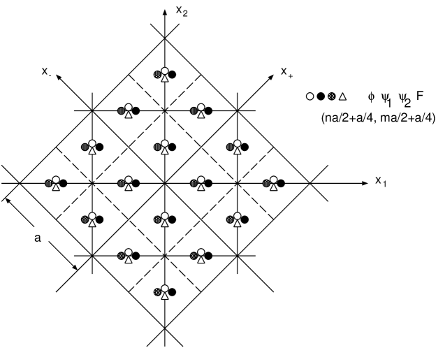
Figure 3: All rescaled fields gather on ($a/4,a/4$) lattice sites.

It should be noticed however that the representation on the lattice of the $D=2$, $N=2$ susy algebra in terms of chiral superfields given below is consistent with either periodic or antiperiodic conditions in the momenta, so that both can be consistently chosen. For a detailed discussion of periodicity, symmetry and hermiticity properties of the chiral and antichiral fields see Appendix A. In the next section chiral and antichiral representations with periodic fields will be used to construct the supersymmetric action on the lattice. This would correspond in Fig. 2 to have the origin shifted of $\frac{a}{4}$ in each direction and all fields sitting on sites $(n\frac{a}{2}+\frac{a}{4},m\frac{a}{2}+\frac{a}{4})$.

In the continuum limit ( $\sin\frac{ap_{\pm}}{2}\to 0$) $\Phi_{A}$ and $\underline{\Phi}_{A}$ coincide if the limit is taken as $ap_{\pm}\to 0$ since $\cos\frac{ap_{\pm}}{4}$ in (4.40) is one in that limit. But if the limit is taken with either $p_{+}$ or $p_{-}$ going to $\frac{2\pi}{a}$ a derivative is generated by the cosine factor. For instance, using for the underlined fields the same notations used in (4.26) we have: $\psi_{1}^{01}=\frac{1}{4}ap_{-}\underline{\psi_{1}^{01}}$. However as a result of the chirality conditions (4.41) the degrees of freedom describing fluctuations around the $p_{\pm}=0$ vacuum are the only independent ones, so the supersymmetry transformations for chiral (and anti-chiral) superfields can be conveniently described in terms of $\underline{\Phi}_{A}$. In order to do that it is convenient to introduce chiral supercharges:

$$Q_{\pm}^{(\pm)}=\frac{1}{2}\left(Q_{\pm}^{(1)}\pm iQ_{\pm}^{(2)}\right),$$ (4.43)

which satisfy the algebra:

$$\left\{Q_{\pm}^{(+)},Q_{\pm}^{(-)}\right\}=2\sin\frac{ap_{\pm}}{2},$$ (4.44)

with all other anticommutators vanishing. The supersymmetry transformations for chiral and anti-chiral superfields are then given respectively in table 2 and 3. In table 3 the components of the anti-chiral superfield are denoted, to distinguish them from the chiral ones, with an over line.

$\begin{array}[]{|l|c|c|c|c|}\hline\cr&\displaystyle Q_{+}^{(+)}&\displaystyle Q_{+}^{(-)}&\displaystyle Q_{-}^{(+)}&\displaystyle Q_{-}^{(-)}\\ \hline\cr\hline\cr\underline{\Phi}(p)&i\underline{\Psi_{1}}(p)&0&i\underline{\Psi_{2}}(p)&0\\ \underline{\Psi_{1}}(p)&0&-2i\sin\frac{ap_{+}}{2}\underline{\Phi}(p)&-F(p)&0\\ \underline{\Psi_{2}}(p)&F(p)&0&0&-2i\sin\frac{ap_{-}}{2}\underline{\Phi}(p)\\ F(p)&0&2\sin\frac{ap_{+}}{2}\underline{\Psi_{2}}(p)&0&-2\sin\frac{ap_{-}}{2}\underline{\Psi_{1}}(p)\\ \hline\cr\end{array}$

Table 2: Chiral $D=N=2$ supersymmetry transformation

$\begin{array}[]{|l|c|c|c|c|}\hline\cr&\displaystyle Q_{+}^{(+)}&\displaystyle Q_{+}^{(-)}&\displaystyle Q_{-}^{(+)}&\displaystyle Q_{-}^{(-)}\\ \hline\cr\hline\cr\bar{\underline{\Phi}}(p)&0&i\bar{\underline{\Psi_{1}}}(p)&0&i\bar{\underline{\Psi_{2}}}(p)\\ \bar{\underline{\Psi_{1}}}(p)&-2i\sin\frac{ap_{+}}{2}\bar{\underline{\Phi}}(p)&0&0&-\bar{F}(p)\\ \bar{\underline{\Psi_{2}}}(p)&0&\bar{F}(p)&-2i\sin\frac{ap_{-}}{2}\bar{\underline{\Phi}}(p)&0\\ \bar{F}(p)&2\sin\frac{ap_{+}}{2}\bar{\underline{\Psi_{2}}}(p)&0&-2\sin\frac{ap_{-}}{2}\bar{\underline{\Psi_{1}}}(p)&0\\ \hline\cr\end{array}$

Table 3: anti-chiral $D=N=2$ supersymmetry transformation

5 N=2 Wess-Zumino model in two dimensions

In the previous section the chiral and anti-chiral representations of the $N=2$, $D=2$ supersymmetry algebra given in tables 2 and 3 have been derived by applying chiral conditions on the reducible representation corresponding to the full superfield expansion. Chiral and anti-chiral representations are irreducible representations, and so they are the building blocks of any supersymmetric action. The result shown in tables 2 and 3 can then be regarded as valid in itself, independently on how it has been derived.

The lattice representations of table 2 and 3 can be obtained from the corresponding representations in the continuum by simply replacing the derivatives $p_{\pm}$ with the sine variables $\sin\frac{ap_{\pm}}{2}$. This implies a lattice spacing $\frac{a}{2}$ (hence a periodicity in momentum space of $\frac{4\pi}{a}$) and consequently a doubling of the degrees of freedom. The doubling can be removed by assuming that all fields are symmetric (or anti-symmetric) in momentum representation under the symmetry operations $p_{\pm}\to\frac{2\pi}{a}-p_{\pm}$. This leads to the conditions (4.41) or (4.42) that in the previous section were obtained by imposing chiral conditions on the full superfield.

The supersymmetry transformations listed in tables 2 and 3 are consistent with all fields being periodic or all anti-periodic with period $\frac{4\pi}{a}$. They are also consistent with fields being symmetric or antisymmetric with respect to $p_{\pm}\to\frac{2\pi}{a}-p_{\pm}$. However if we assume that anti-chiral fields are hermitian conjugate of the chiral ones, so that:

$$\underline{\Phi}_{A}^{\dagger}(p)=\bar{\underline{\Phi}}_{A}(-p),$$ (5.1)

then the periodicity with period $\frac{4\pi}{a}$ in the momenta implies that chiral and anti-chiral fields are both symmetric or both antisymmetric with respect to $p_{\pm}\to\frac{2\pi}{a}-p_{\pm}$. On the other hand anti periodicity in the momenta requires chiral and anti-chiral fields to have opposite symmetry properties with respect to $p_{\pm}\to\frac{2\pi}{a}-p_{\pm}$ as in (4.41) and (4.42). All these choices are consistent with the supersymmetry transformations. However writing the action imposes some restrictions. The Lagrangian density has to be periodic with period $\frac{4\pi}{a}$ in each integrated momentum. An antiperiodic density would lead to a vanishing action when integrated over a $\frac{8\pi}{a}$ interval. Since each integrated momentum is associated to just one field the anti-periodic option for the fields should be discarded. Let us now consider the symmetry under $p_{\pm}\to\frac{2\pi}{a}-p_{\pm}$. Let $L$ be the Lagrangian density and $p$ an integration variable, namely the $+$ or $-$ component of a field’s momentum. If we use $dp$ as integration measure the Lagrangian density should be symmetric (and not antisymmetric) under $p\to\frac{2\pi}{a}-p$. In fact, if $L(\cdots,\frac{2\pi}{a}-p,\cdots)=L(\cdots,p,\cdots)$ we have:

$$\int_{-\frac{\pi}{a}}^{\frac{3\pi}{a}}dpL(\cdots,p,\cdots)=2\int_{-\frac{\pi}{a}}^{\frac{\pi}{a}}dpL(\cdots,p,\cdots),$$ (5.2)

whereas the l.h.s. of (5.2) vanishes if $L(\cdots,\frac{2\pi}{a}-p,\cdots)=-L(\cdots,p,\cdots)$ . If all the $p$ dependence in $L$ is contained in the corresponding fields and in the delta function expressing the sine momentum conservation, then all fields should be symmetric under $p_{\pm}\to\frac{2\pi}{a}-p_{\pm}$. However if we use $\hat{p}=\frac{2}{a}\sin\frac{ap}{2}$ as integration variable and $d\hat{p}=\cos\frac{ap}{2}dp$ as integration volume the extra antisymmetric cosine factor will require an antisymmetric Lagrangian density to re-establish the symmetry. In this case all fields should be antisymmetric under $p_{\pm}\to\frac{2\pi}{a}-p_{\pm}$.

The two choices are equivalent: in the former case the cosine factor is included in the field definition, in the latter case in the integration volume and multiplication by a factor $\cos\frac{ap_{+}}{2}\cos\frac{ap_{-}}{2}$ changes the symmetry property of the field under $p_{\pm}\to\frac{2\pi}{a}-p_{\pm}$ while not affecting its continuum limit.

5.1 The kinetic term

In our lattice formulation the quadratic terms in the action enjoy a unique property, as already discussed in the one dimensional case of ref. [20]. The sine momentum conservation

$$\sin\frac{ap_{\pm}}{2}+\sin\frac{aq_{\pm}}{2}=0,$$ (5.3)

has two separate solutions, namely:

$$p_{\pm}+q_{\pm}=0,~{}~{}~{}~{}~{}~{}~{}~{}~{}~{}\textrm{and}~{}~{}~{}~{}~{}~{}~{}~{}~{}~{}~{}~{}~{}p_{\pm}-q_{\pm}=\frac{2\pi}{a},~{}~{}~{}~{}~{}~{}~{}~{}~{}~{}~{}~{}~{}~{}~{}~{}~{}~{}(\textrm{mod}\frac{4\pi}{a}),$$ (5.4)

so that the delta functions expressing the sine conservation laws can be replaced, preserving all the symmetries of the theory, by delta functions with the argument linear in the momenta, namely by:

$$\delta^{(s)}(p+q)\equiv\prod_{i=\pm}\frac{1}{2}\left[\delta(p_{i}+q_{i})+\delta(p_{i}-q_{i}+\frac{2\pi}{a})\right],~{}~{}~{}~{}~{}~{}~{}~{}(\textrm{mod}\frac{4\pi}{a}).$$ (5.5)

The kinetic term of the supersymmetric Wess-Zumino action can then be written on the lattice using the same construction as in the continuum:

$$S_{K} = \int_{-\frac{\pi}{a}}^{\frac{3\pi}{a}}dp_{+}dp_{-}dq_{+}dq_{-}\delta^{(s)}(p+q)Q_{+}^{(-)}Q_{-}^{(-)}Q_{+}^{(+)}Q_{-}^{(+)}\{\bar{\underline{\Phi}}(p)\underline{\Phi}(q)\}$$ (5.6)

$$= \int_{-\frac{\pi}{a}}^{\frac{3\pi}{a}}dp_{+}dp_{-}dq_{+}dq_{-}\delta^{(s)}(p+q)\left[-4\bar{\underline{\Phi}}(p)\sin\frac{aq_{+}}{2}\sin\frac{aq_{-}}{2}\underline{\Phi}(q)-\bar{F}(p)F(q)\right.$$

$$\left.+2\bar{\underline{\Psi_{2}}}(p)\sin\frac{aq_{+}}{2}\underline{\Psi_{2}}(q)+2\bar{\underline{\Psi_{1}}}(p)\sin\frac{aq_{-}}{2}\underline{\Psi_{1}}(q)\right].$$

The invariance of the action $S_{K}$ under all the supersymmetry transformations generated by $Q_{\pm}^{(\pm)}$ is assured, as in the continuum, by the algebra of the $Q$’s and by the momentum conservation (5.5), which is equivalent to (5.3).

We assume that all fields satisfy the symmetry condition (4.41), so that in each variable the contribution of the integration in the intervals $(-\frac{\pi}{a},\frac{\pi}{a})$ and $(\frac{\pi}{a},\frac{3\pi}{a})$ coincide and we get:

$$S_{K} = 4\int_{-\frac{\pi}{a}}^{\frac{\pi}{a}}dp_{+}dp_{-}dq_{+}dq_{-}\delta(p_{+}+q_{+})\delta(p_{-}+q_{-})\left[-4\bar{\underline{\Phi}}(p)\sin\frac{aq_{+}}{2}\sin\frac{aq_{-}}{2}\underline{\Phi}(q)\right.$$ (5.7)

$$\left.-\bar{F}(p)F(q)+2\bar{\underline{\Psi_{2}}}(p)\sin\frac{aq_{+}}{2}\underline{\Psi_{2}}(q)+2\bar{\underline{\Psi_{1}}}(p)\sin\frac{aq_{-}}{2}\underline{\Psi_{1}}(q)\right].$$

The advantage of using directly the momentum conservation (5.5), rather than the sine conservation, is that the action (5.6) can be formulated in coordinate representation by a simple Fourier transform. Using (4.41) we find:

$$S_{K} = 4\pi^{2}\sum_{x_{\pm}=\frac{n_{\pm}a}{2}}\left[\bar{\underline{\Phi}}(x)\Delta_{+}\Delta_{-}\underline{\Phi}(x)-\bar{F}(x)F(x)-i\bar{\underline{\Psi_{2}}}(x)\Delta_{+}\underline{\Psi_{2}}(x)\right.$$ (5.8)

$$\left.-i\bar{\underline{\Psi_{1}}}(x)\Delta_{-}\underline{\Psi_{1}}(x)\right],$$

where

$$\Delta_{+}\underline{\Phi}_{A}(x) = \underline{\Phi}_{A}(x_{+}+\frac{a}{2},x_{-})-\underline{\Phi}_{A}(x_{+}-\frac{a}{2},x_{-}),$$

$$\Delta_{-}\underline{\Phi}_{A}(x) = \underline{\Phi}_{A}(x_{+},x_{-}+\frac{a}{2})-\underline{\Phi}_{A}(x_{+},x_{-}-\frac{a}{2}).$$ (5.9)

The fields in action (5.8) must satisfy the “chiral” conditions (4.41), which in coordinate representation are:

$$\underline{\Phi}_{A}(x_{+},x_{-})=(-1)^{n_{+}}\underline{\Phi}_{A}(-x_{+},x_{-})=(-1)^{n_{-}}\underline{\Phi}_{A}(x_{+},-x_{-})=(-1)^{n_{+}+n_{-}}\underline{\Phi}_{A}(-x_{+},-x_{-}),$$ (5.10)

with $x_{\pm}=\frac{an_{\pm}}{2}$. Through eq.s (5.10) the degrees of freedom in four different points, obtained by reflection with respect to the $x_{+}=0$ and $x_{-}=0$ axis, are identified and in spite of the $a/2$ lattice spacing the density of independent degrees of freedom is the same as in a lattice with spacing $a$. The lattice is not smoothly mapped into the coordinate space in the continuum limit as eq.s (5.10) have no continuum limit. To make contact with continuum space-time one has to separate long wavelength modes ( around $p_{\pm}=0$) from the short wavelength ones (around $p_{\pm}=\frac{2\pi}{a}$) using (4.41). In other words one has to consider the action (5.7), where all fields are defined in the momentum region $-\frac{\pi}{a}\leq p_{\pm}\leq\frac{\pi}{a}$. The Fourier transform over a $\frac{2\pi}{a}$ interval will produce fields in coordinate representation defined on a lattice with spacing $a$, which can be identified with the continuum space-time in the continuum limit. With this lattice we will show in Appendix that the translational invariance, which is broken by the sine conservation law, is recoverd in the continuum limit. However the symmetric finite difference operators $\sin\frac{ap_{\pm}}{2}$ are not periodic with period $\frac{2\pi}{a}$ , so the resulting action in coordinate representation will be highly non-local as in the SLAC derivative case.

The kinetic term (5.8) instead is local on the $a/2$ lattice, modulo the $x\to-x$ symmetry (5.10), which also breaks the translational invariance.

All fields appearing in (5.8) are dimensionless. When the continuum limit is taken some powers of $a$ appear and fields need to scale with $a$ for the limit to be smooth. More precisely we have that powers of $a$ are generated by $\sum_{n_{\pm}}\to\frac{1}{a^{2}}\int dx_{+}dx_{-}$ and by $\Delta_{\pm}\to a\frac{\partial}{\partial x_{\pm}}$. In order for these powers of $a$ to be absorbed fields have to rescale with $a$, the rescaled fields thus acquiring the standard dimensions fields. So we have:

$$\underline{\Phi}(x)\to\varphi(x),~{}~{}~{}~{}\frac{1}{\sqrt{a}}\underline{\Psi_{i}}(x)\to\psi_{i}(x),~{}~{}~{}~{}\frac{1}{a}F(x)\to f(x)$$ (5.11)

where the fields at the right sides are the rescaled dimensional fields, to be identified with the ones in the continuum limit.

5.2 Mass term and interaction terms

As in the continuum formulation mass and interaction term have a different structure with respect to the kinetic term, as they made by the sum of two terms, one involving only chiral fields, the other only anti-chiral fields. The general structure is:

$$S_{n} = \int\prod_{j=1}^{n}d^{2}p_{j}V_{n}(p)Q_{+}^{(+)}Q_{-}^{(+)}\{\underline{\Phi}(p_{1})\underline{\Phi}(p_{2})\cdots\underline{\Phi}(p_{n})\}+\textrm{h.c.}$$

$$= \int\prod_{j=1}^{n}d^{2}p_{j}V_{n}(p)n\left[iF(p_{1})\prod_{j=2}^{n}\underline{\Phi}(p_{j})+(n-1)\underline{\Psi_{2}}(p_{1})\underline{\Psi_{1}}(p_{2})\prod_{j=3}^{n}\underline{\Phi}(p_{j})\right]+\textrm{h.c.},$$

where $V_{n}(p)$ is an integration volume to be discussed shortly which includes the delta function of momentum conservation and is symmetric under permutations of the $n$ momenta.

In the case of the mass term we set $n=2$ in (5.2). Moreover, being a quadratic interaction, we can simply choose, as in the kinetic term, the following integration volume:

$$V_{2}(p)=ma^{2}\delta^{(s)}(p_{1}+p_{2})=ma^{2}\prod_{i=\pm}\frac{1}{2}\left[\delta(p_{1i}+p_{2i})+\delta(p_{1i}-p_{2i}+\frac{2\pi}{a})\right]~{}~{}~{}~{}\textrm{mod.}\frac{4\pi}{a},$$ (5.13)

where $m$ is an dimensionless mass parameter and the factor $a^{2}$ is introduced for dimensional reasons so that $S_{2}$ is dimensionless. So the mass term in momentum representation is:

$$S_{2}=ma^{2}\int\prod_{j=1}^{2}d^{2}p_{j}~{}\delta^{(s)}(p_{1}+p_{2})\left[iF(p_{1})\underline{\Phi}(p_{2})+\underline{\Psi_{2}}(p_{1})\underline{\Psi_{1}}(p_{2})\right],$$ (5.14)

where as usual the “chiral” conditions (4.41) hold. As in the kinetic term the action is local in coordinate representation, but with the non-local $x\to-x$ symmetry (5.10):

$$S_{2}=4m\pi^{2}\sum_{x_{\pm}=\frac{an_{\pm}}{2}}\left[iF(x)\underline{\Phi}(x)+\underline{\Psi_{2}}(x)\underline{\Psi_{1}}(x)\right].$$ (5.15)

To make contact with the continuum theory the lattice fields must be rescaled as in (5.11) and the resulting $a$ factors are absorbed in the parameter $m$ leading to the dimensional mass parameter $M=\frac{m}{a}$.

In the interaction terms ($n\geq 3$) the integration volume $V_{n}(p)$ must contain the delta function expressing the sine momentum conservation. We define then:

$$V_{n}(p)=a^{2n}~{}g_{n}~{}G_{n}(p)~{}\delta^{(2)}\left(\sin\frac{ap_{1}}{2}+\sin\frac{ap_{2}}{2}+\cdots+\sin\frac{ap_{n}}{2}\right),$$ (5.16)

where $g_{n}$ is a dimensionless coupling constant and $G_{n}(p)$ can be in principle any function periodic in each momentum component with period $\frac{4\pi}{a}$, symmetric under permutations of the momenta and invariant under the substitution $p_{i\pm}\to\frac{2\pi}{a}-p_{i\pm}$. We choose $G_{n}(p)$ to be $1$ in the continuum limit, namely when all momentum components $p_{i\pm}$ are either zero or $\frac{2\pi}{a}$. We also choose $G_{n}(p)$ to vanish whenever a momentum component $p_{i\pm}$ is equal to $\pm\frac{\pi}{a}$ to avoid the integration volume to blow up as an effect of the sines in the delta function. The minimal way to satisfy all these requirements is to choose:

$$G_{n}(p)=C_{n}(p),$$ (5.17)

where

$$C_{n}(p)\equiv\prod_{j=1}^{n}|\cos\frac{ap_{j+}}{2}\cos\frac{ap_{j-}}{2}|.$$ (5.18)

Clearly any positive power of $C_{n}(p)$ ( for instance $G_{n}(p)=C_{n}^{2}(p)$) would equally satisfy all symmetry requirement.

As an example we give explicitly the cubic interaction term. Setting $n=3$ in (5.2) and using (5.16) and (5.17) we have:

$$S_{3} = 3a^{6}g_{3}\int\prod_{j=1}^{3}d^{2}p_{j}|\cos\frac{ap_{j+}}{2}\cos\frac{ap_{j-}}{2}|~{}\delta^{(2)}\left(\sin\frac{ap_{1}}{2}+\sin\frac{ap_{2}}{2}+\sin\frac{ap_{3}}{2}\right)$$ (5.19)

$$\left[iF(p_{1})\underline{\Phi}(p_{2})\underline{\Phi}(p_{3})+2\underline{\Psi_{2}}(p_{1})\underline{\Psi_{1}}(p_{2})\underline{\Phi}(p_{3})\right]+\textrm{h.c.}.$$

The continuum limit of (5.19) is obtained by taking $a\to 0$, namely $|ap_{j}|\ll 1$. In principle we should also consider the regions where one or more components of the momenta are close to $\frac{2\pi}{a}$, but thanks to (4.41) these regions are just copies of the $p_{j}=0$ region and they only give an overall multiplicative factor. All fields in (5.19) are dimensionless, so a rescaling is needed to make contact with the continuum fields:

$$a^{2}\underline{\Phi}(p)\to\varphi(p),~{}~{}~{}~{}a^{\frac{3}{2}}\underline{\Psi_{i}}(p)\to\psi_{i}(p),~{}~{}~{}~{}aF(p)\to f(p),$$ (5.20)

which differ from (5.11) because of the different dimensionality in the continuum of fields in coordinate and momentum representation. Neglecting overall numerical factors the continuum limit of (5.19) is then:

$$S_{3}\to g^{(c)}_{3}\int\prod_{j=1}^{3}d^{2}p_{j}\delta^{(2)}\left(p_{1}+p_{2}+p_{3}\right)\left[if(p_{1})\varphi(p_{2})\varphi(p_{3})+2\psi_{2}(p_{1})\psi_{1}(p_{2})\varphi(p_{3})\right]+\textrm{h.c.},$$ (5.21)

where $g^{(c)}_{3}=\frac{g_{3}}{a^{3}}$ is the dimensional coupling constant of the continuum theory.

As in the one dimensional case of ref. [20] the coordinate representation of the interaction terms involves non-locality, due to the sine momentum conservation. This can be formalized by introducing, as in [20], a new non-local product of fields, the star product. With respect to this product the symmetric finite difference operator satisfies the Leibnitz rule, leading in momentum space to the sine momentum conservation. This will be explained in detail in the next section.

Another affect of the sine conservation law is that it breaks the translational invariance at finite lattice spacing. In the continuum limit, however, the translational invariance is recovered (see Appendix B).

6 Star product in two dimensions

With ordinary momentum conservation the convolution of a product of two field $F\cdot G$ is defined as a result of additive momentum $p=p_{1}+p_{2}$ under the product:

$$(F\cdot G)(p)=\left(\frac{a}{2\pi}\right)^{2}\int d^{2}p_{1}d^{2}p_{2}F(p_{1})G(p_{2})\delta^{(2)}(p-p_{1}-p_{2}).$$ (6.1)

In coordinate space this amounts to the ordinary local product:

$$(F\cdot G)(x)=F(x)G(x).$$ (6.2)

On the lattice the standard momentum conservation is replaced by the lattice (sine) momentum conservation, which means that $\hat{p}_{\pm}=\frac{2}{a}\sin\frac{ap_{\pm}}{2}$ is the additive quantity when taking the product of two fields. This amounts to changing the definition of the “dot” product to that of a “star” product defined in momentum space as:

$$(F*G)(p)=\left(\frac{a}{2\pi}\right)^{2}\int d^{2}\hat{p}_{1}d^{2}\hat{p}_{2}F(p_{1})G(p_{2})\delta^{(2)}(\hat{p}-\hat{p}_{1}-\hat{p}_{2})$$ (6.3)

As we shall see this product is not anymore local in coordinate space but satisfies the Leibnitz rule with respect to the symmetric difference operator $\Delta_{\pm}$. This is easily checked in the momentum representation. An operation of $\Delta_{\pm}$ in the coordinate space corresponds in momentum space to multiplication by $\hat{p}_{\pm}=\frac{2}{a}\sin\frac{ap_{\pm}}{2}$, so that the lattice momentum conservation leads to the Leibnitz rule on the lattice momentum space:

$$\hat{p}_{\pm}~{}(F*G)(p)=\left(\frac{a}{2\pi}\right)^{2}\int d^{2}\hat{p}_{1}\,d^{2}\hat{p}_{2}\left[\hat{p}_{1\pm}F(p_{1})~{}G(p_{2})+F(p_{1})\,\hat{p}_{2\pm}G(p_{2})\right]\delta^{(2)}(\hat{p}-\hat{p}_{1}-\hat{p}_{2}).$$ (6.4)

It is thus natural to expect that Leibnitz rule will be satisfied on the corresponding coordinate space where the lattice momentum conservation is satisfied. On this new coordinate space the product of fields is modified. We call this new product as a new type of star $*$-product and it was proposed in our previous paper[20]. Similar proposal[16] was given at the early investigation of lattice supersymmetry following to the suggestion of the lattice momentum conservation of Dondi and Nicolai[7].

Explicit form of the coordinate representation of the star product is given by

$$(F*G)(x) = F(x)*G(x)=a^{2}\int\frac{d^{2}\hat{p}}{(2\pi)^{2}}\,e^{-ipx}~{}(F*G)(p)$$ (6.5)

$$= \int_{-\frac{\pi}{2}}^{\frac{3\pi}{2}}d^{2}\tilde{p}~{}\cos\tilde{p}_{+}\cos\tilde{p}_{-}~{}e^{-ipx}\int_{-\frac{\pi}{2}}^{\frac{3\pi}{2}}\frac{d^{2}\tilde{p}_{1}}{(2\pi)^{2}}\frac{d^{2}\tilde{p}_{2}}{(2\pi)^{2}}\cos\tilde{p}_{1+}\cos\tilde{p}_{1-}\,\cos\tilde{p}_{2+}\cos\tilde{p}_{2-}$$

$$\times\int_{-\infty}^{\infty}\frac{d^{2}\tau}{(2\pi)^{2}}e^{i{\tau}\cdot(\sin\tilde{p}-\sin\tilde{p}_{1}-\sin\tilde{p}_{2})}\sum_{y_{\pm},z_{\pm}}e^{i(m\cdot\tilde{p}_{1}+l\cdot\tilde{p}_{2})}F(y)G(z)$$

$$= \int_{-\infty}^{\infty}d^{2}\tau J_{n_{+}\pm 1}({\tau}_{+})J_{n_{-}\pm 1}({\tau}_{-})$$

$$\times\sum_{m_{\pm},l_{\pm}}J_{m_{+}\pm 1}({\tau}_{+})J_{m_{-}\pm 1}({\tau}_{-})J_{l_{+}\pm 1}(\tau_{+})J_{l_{-}\pm 1}(\tau_{-})F(y)G(z),$$

where $\tilde{p}_{\pm}=\frac{ap_{\pm}}{2}$, and $x_{\pm}=\frac{n_{\pm}a}{2},y_{\pm}=\frac{m_{\pm}a}{2},z_{\pm}=\frac{l_{\pm}a}{2}$ should be understood and the integration variable is not $p_{\pm}$ but $\hat{p}_{\pm}$.

The lattice delta function is parameterized by $\tau_{\pm}$

$$\delta^{(2)}\left(\frac{2}{a}\sin\tilde{p}_{i}\right)=\left(\frac{a}{4\pi}\right)^{2}\int^{\infty}_{-\infty}d^{2}\tau e^{i({\tau}_{+}\sin\tilde{p}_{i+}+\tau_{-}\sin\tilde{p}_{i-})}.$$ (6.6)

$J_{n}(\tau_{\pm})$ is a Bessel function defined as

$$J_{n}(\tau_{\pm})=\frac{1}{2\pi}\int_{\alpha}^{2\pi+\alpha}e^{i(n\theta-\tau_{\pm}\sin\theta)}d\theta,$$ (6.7)

and we use the following notation:

$$J_{n\pm 1}(\tau)=\frac{1}{2}(J_{n+1}(\tau)+J_{n-1}(\tau)).$$ (6.8)

It is obvious that the star product is commutative:

$$F(x)*G(x)=G(x)*F(x).$$ (6.9)

We can now explicitly check how the difference operator acts on the star product of two lattice fields and find that the difference operator action on the star product indeed satisfies Leibnitz rule:

$$i\Delta_{\pm}(F(x)*G(x)) =a^{2}\int\frac{d\hat{p}}{(2\pi)^{2}}~{}i\Delta_{x_{\pm}}~{}e^{-ipx}~{}(F*G)(p)$$

$$=\left(\frac{a^{2}}{4}\right)^{2}\int d^{2}\hat{p}~{}e^{-ipx}\sum_{y_{\pm},z_{\pm}}\int\frac{d^{2}\hat{p}_{1}}{(2\pi)^{2}}\frac{d^{2}\hat{p}_{2}}{(2\pi)^{2}}~{}e^{ip_{1}y+ip_{2}z}$$

$$~{}~{}~{}~{}~{}~{}~{}\times\left((i\Delta_{y_{\pm}}~{}F(y))G(z)~{}+~{}F(y)~{}(i\Delta_{z_{\pm}}~{}G(z))\right)~{}\delta^{(2)}(\hat{p}-\hat{p}_{1}-\hat{p}_{2})$$

$$=(i\Delta_{\pm}F(x))*G(x)+F(x)*(i\Delta_{\pm}G(x)).$$ (6.10)

We can now generalize the definition of the star product for n fields as:

$$F_{1}(x+b_{1})*F_{2}(x+b_{2})* \cdots *F_{n}(x+b_{n})=\int^{\infty}_{-\infty}d^{2}\tau J_{n_{+}\pm 1}(\tau_{+})J_{n_{-}\pm 1}(\tau_{-})$$

$$\sum_{m_{1}\pm,\cdots,m_{n}\pm}\left(\prod_{j=1}^{n}J_{m_{j}+\pm 1}(\tau_{+})J_{m_{j}-\pm 1}(\tau_{-})F_{j}(y_{j}+b_{j})\right),$$

where $\frac{2x_{\pm}}{a}=n_{\pm},\frac{2y_{\pm}}{a}=m_{j\pm}$. It should be noted that interaction terms includes the product a higher powers of lattice fields. As we can see from the above expression the kernel of an interaction term includes an integration of Bessel functions which is integrable. Thus a possible nonlocality of interaction terms is expected to be mild due to the integrability of the kernel.

The kinetic term of $N=2$ lattice Wess-Zumino action in two dimensions can be written with the star product form as:

$$S_{K}~{}=~{}\sum_{x_{\pm}}\{-\bar{\phi}(x)*\Delta_{+}\Delta_{-}\phi(x)-\bar{F}(x)*F(x)+\bar{\psi}_{2}(x)*\Delta_{+}\psi_{2}(x)+\bar{\psi}_{1}(x)*\Delta_{-}\psi_{1}(x)\}$$ (6.12)

The interaction term can be given as

$$S_{I}~{}=~{}\sum_{x_{\pm}}\{iF(x)*(\phi(x))^{n-1}+\psi_{2}(x)*\psi_{1}(x)*(\phi(x))^{n-2}\}.$$ (6.13)

These actions are exactly $N=2$ supersymmetry invariant on the star product since the difference operator satisfies Leibnitz rule.

7 Conclusion and Discussions

In this paper we have proposed a formulation which solves two of the major difficulties in the lattice supersymmetry: (1) the breaking of the Leibnitz rule by the finite difference operator and (2) the doubling problem of chiral fermions.

In order to solve the problem (1) and yet keep an exact lattice supersymmetric formulation, we take a stance of choosing the sine of the momentum, rather than the momentum itself, as conserved quantity on the lattice. As mentioned in the introduction this agrees with lattice periodicity in momentum space but leads in coordinate space to a nonlocal interaction terms and to a loss of finite lattice translational invariance. The problem (2) is solved by introducing a half lattice structure and identifying species doublers as super partners for fermions and bosons. Since the species doublers are identified as physical super partners there is essentially no chiral fermion problem.

The basic structure of the lattice supersymmetry transformation which we have proposed here can be seen by a coordinate representation of the simplest supersymmetric model in one dimension. In order to accommodate lattice supersymmetry transformations it is crucial to introduce a lattice with spacing $\frac{a}{2}$ together with an alternating sign change. In momentum space the alternating sign multiplication corresponds to a momentum shift of $\frac{2\pi}{a}$, namely to a species doubler state. Thus the species doubler states are mixed under the supersymmetry transformation.

The lattice version of $N=2$ exact supersymmetry algebra including superderivative in one and two dimensions are fully reconstructed especially in the momentum space. We found algebraic chiral conditions which are fundamentally connected with species doubling structure of chiral fermions on the lattice. In particular the irreducible representations of chiral and anti-chiral fields turn out to be fully symmetric or antisymmetric combinations of the original field and the species doubler field in each momentum direction. Thus the chiral condition truncates the reducible part of unnecessary doubler fields. In two dimensional $N=2$ the 16 fields of the complete superfield (including doublers of fermion and boson) are truncated 4 states by the chiral conditions forming an irreducible representation. The chiral conditions require to define newly rescaled fields which have different periodicity from the original fields in momentum space. The original fields are scattered and separated by $\frac{a}{4}$ spacing. The chiral condition has the effect of defining new fields that gather into the same site of ($\frac{a}{4},\frac{a}{4}$) lattice, having half lattice spacing into each light cone direction.

The one dimensional action derived heuristically in the previous paper [20] is derived as a chiral super charge exact form of the super fields together with the lattice version of sine momentum conservation. On the other hand the two dimensional $N=2$ supersymmetric Wess-Zumino action can be derived as a chiral super charge exact form of the chiral and anti-chiral super fields. It would be interesting to reveal the fundamental difference of the formulations between one and two dimensions: In one dimension all the species doublers are used to construct the action while 1/4 species doublers out of $4\times 4$=16 are truncated into 4 by the chiral condition and 4+4=8 chiral and anti-chiral fields are needed for the two dimensional Wess-Zumino action. The invariance under $N=2$ exact lattice supersymmetry of the actions is assured by the nil-potency of chiral super charges and by the lattice momentum conservation.

Since the algebra has a lattice periodicity in the momentum space, it is natural that delta function should have the same periodicity and thus leading to the lattice sine momentum conservation. The corresponding coordinate representation of the formulation defines a new type of product which we called a star product[20]. This product has a nonlocal nature but expected to have milder non-locality than the non-locality generated by the SLAC type derivative since the kernel of the interaction terms are expressed by Bessel functions and thus they are integrable. It is important to note that the difference operator satisfies the Leibnitz rule on star product fields. Thus exact supersymmetry invariance on the coordinate space with the star product fields is assured in parallel to the momentum representation.

The periodic momentum conservation unavoidably enforces us to introduce a non-locality and non-translational invariance into the formulation. As we argued in the introduction the non-locality would be unavoidable in the formulation if we strictly require the exact lattice supersymmetry for the formulation. We consider that the lattice version of sine momentum conservation is the best possible choice if we keep strictly an exact lattice supersymmetry. It is shown that the translational invariance is recovered in the continuum limit.

In solving lattice chiral fermion problem, exponentially damping non-locality was accepted and an modification of lattice chiral transformation was introduced. By breaking one of presumed conditions of No-Go theorem[36] the satisfactory solution for the lattice chiral fermion was obtained. We may take a similar stance for solving the lattice supersymmetry. In other wards we accept the breakdown of locality and translational invariance in the lattice supersymmetry formulation and then expect that the locality and translational invariance recovers harmlessly in the continuum limit. We have confirmed that this recovery of the translational invariance is realized even with quantum corrections from dimensional arguments in the Appendix. It is, however, important to see if this is the case even in the nonperturbative regime. We may say that it is similar to expect the recovery of Lorentz invariance in the continuum limit. It is also important to investigate carefully if the exactness of the lattice supersymmetry is kept even at the quantum level. In our previous paper I[20] we showed that the lattice supersymmetry is kept at the one loop quantum level. It is also necessary to investigate a quantum level exactness of the lattice supersymmetry given in this paper. The extension of the formulation given here into higher dimensions and also gauge theory is obviously important. The question of feasibility for numerical evaluation may be important. In this paper we have formulated Minkowsky version of lattice supersymmetry. It may be neccessary to reformulate in the Euclidean lattice for numerical simulation.

Acknowledgments N.K. would like to thank K. Asaka, Y. Kondo, E. Giguere for useful discussions. This work was supported in part by Japanese Ministry of Education, Science, Sports and Culture under the grant number 22540261 and also by the research funds of Insituto Nazionale di Fisica Nucleare (INFN). I.K. is supported in part by the Deutsche Forschungsgemeinschaft (Sonder-forschungsbereich / Transregio 55) and the Research Executive Agency (REA) of the European Union under Grant Agreement number PITN-GA-2009-238353 (ITN STRONGnet).

Appendix

Appendix A Periodicity, hermiticity and symmetry properties of lattice fields

In this appendix we summarize and review the periodicity properties of the lattice fields in the momentum representations, and how these are related to hermiticity and symmetry properties under $p_{\pm}\rightarrow\frac{2\pi}{a}-p_{\pm}$. These properties have been discussed and used through the paper and are collected here for the reader’s convenience.

A.1 Periodicity in $p_{\pm}$

In the present approach each lattice field $\Phi_{A}$ is defined on a lattice with spacing $\frac{a}{2}$ defined by

$$\vec{x}_{\pm}=\{(n+b_{A})\frac{a}{2},~{}(m+c_{A})\frac{a}{2}\},~{}~{}~{}~{}~{}~{}n,m\in{\bf Z},$$ (A.1)

where $b_{A}$ and $c_{A}$ represent the shift of the lattice on which the field $\Phi_{A}$ is defined with respect to the origin of the coordinate space. In the formulation of chiral lattice supersymmetry given in the present paper it is not possible to set all $b_{A}$ and $c_{A}$ to zero, because supersymmetry transformations are defined in terms of symmetric finite differences of spacing $\frac{a}{2}$ as shown in (4.16). As a result, if we set the shifts $b$ and $c$ equal to zero for the first component $\Phi$ of the superfield, the different fields of the $N=2$ supermultiplet are effectively defined on a lattice with spacing $\frac{a}{4}$, as shown in fig. 2. In the momentum representation a field $\Phi_{A}$ defined on the lattice (A.1) is periodic in the momenta with period $\frac{4\pi}{a}$ up to a phase that depends on the shifts $b_{A}$ and $c_{A}$. more precisely we have:

$$\Phi_{A}(p_{+}+\frac{4\pi}{a},p_{-}) = e^{2i\pi b_{A}}\Phi_{A}(p_{+},p_{-})$$

$$\Phi_{A}(p_{+},p_{-}+\frac{4\pi}{a}) = e^{2i\pi c_{A}}\Phi_{A}(p_{+},p_{-})$$ (A.2)

With the choice of shifts corresponding to the lattice of fig. 2 the phases at the r.h.s. of (A.2) are just $\pm 1$, and the periodicity conditions of the different field are the ones given in (LABEL:period2), which we reproduce here for convenience and we denote as case A:

$$\Phi(p_{+},p_{-})= \Phi(p_{+}+\frac{4\pi}{a},p_{-})=\Phi(p_{+},p_{-}+\frac{4\pi}{a}),$$

$$\framebox{Case A}\qquad\Psi_{1}(p_{+},p_{-})= -\Psi_{1}(p_{+}+\frac{4\pi}{a},p_{-})=\Psi_{1}(p_{+},p_{-}+\frac{4\pi}{a}),$$

$$\Psi_{2}(p_{+},p_{-})= \Psi_{2}(p_{+}+\frac{4\pi}{a},p_{-})=-\Psi_{2}(p_{+},p_{-}+\frac{4\pi}{a}),$$

$$F(p_{+},p_{-})= -F(p_{+}+\frac{4\pi}{a},p_{-})=-F(p_{+},p_{-}+\frac{4\pi}{a}),$$

The important point here is that while the relative shifts $b_{A}-b_{A^{\prime}}$ and $c_{A}-c_{A^{\prime}}$ of the different component fields are determined by the algebraic structure of supersymmetry transformations, the latter allows an arbitrary choice for the origin of the $\frac{a}{4}$ lattice of fig. 2. The periodicity conditions (LABEL:period2app) correspond to the lattice origin coinciding with the site of a $\Phi$ field, namely to the first component of the superfield $\Phi(x_{+},x_{-})$ being defined on the lattice of sites $(\frac{n}{2},\frac{m}{2})$. But other choices are equally consistent with the algebra: in particular we can choose the last component $F$ to be defined on the lattice of sites $(\frac{n}{2},\frac{m}{2})$. This corresponds, with respect to the previous choice, to a shift of the origin of $\frac{a}{4}$ in each light cone direction. In momentum representation this means exchanging periodicity with antiperiodicity in (LABEL:period2app), namely (case B):

$$\Phi(p_{+},p_{-})= -\Phi(p_{+}+\frac{4\pi}{a},p_{-})=-\Phi(p_{+},p_{-}+\frac{4\pi}{a}),$$

$$\framebox{Case B}\qquad\Psi_{1}(p_{+},p_{-})= \Psi_{1}(p_{+}+\frac{4\pi}{a},p_{-})=-\Psi_{1}(p_{+},p_{-}+\frac{4\pi}{a}),$$

$$\Psi_{2}(p_{+},p_{-})= -\Psi_{2}(p_{+}+\frac{4\pi}{a},p_{-})=\Psi_{2}(p_{+},p_{-}+\frac{4\pi}{a}),$$

$$F(p_{+},p_{-})= F(p_{+}+\frac{4\pi}{a},p_{-})=F(p_{+},p_{-}+\frac{4\pi}{a}),$$

(A.4)

In terms of the rescaled fields $\underline{\Phi}_{A}$ defined in (4.40), which are the relevant ones for writing the chiral conditions, the periodicity conditions are particularly simple. In coordinate representation all fields $\underline{\Phi}_{A}$ are on the same sites of a lattice with spacing $\frac{a}{2}$. In the case A this is given by the sites of coordinates $(\frac{na}{2}+\frac{a}{4},\frac{ma}{2}+\frac{a}{4})$ and is represented in fig. 3. In the case B the lattice is obtained from case A with a shift of $\frac{a}{4}$ in each light cone direction, it includes the origin and is given by the sites $(\frac{an}{2},\frac{am}{2})$. In momentum representation all fields $\underline{\Phi}_{A}$ have the same periodicity properties: in case A they are all antiperiodic with period $\frac{4\pi}{a}$ in $p_{+}$ and $p_{-}$, in case B on the other hand they are all periodic.

A.2 Hermiticity and symmetry properties under $p_{\pm}\rightarrow\frac{2\pi}{a}-p_{\pm}$

We have assumed all through the paper that the fields $\Phi_{A}(x)$ in coordinate representation are real. In momentum representation this means:

$$\Phi^{\dagger}_{A}(p)=\Phi_{A}(-p).$$ (A.5)

On the other hand we discussed in Section 4 that the chiral and anti-chiral parts of the component fields $\underline{\Phi}_{A}$ are given respectively by the symmetric and antisymmetric parts with respect to the symmetry transformations $p_{\pm}\rightarrow\frac{2\pi}{a}-p_{\pm}$ as shown in (4.41) and (4.42). We want to show now how the hermiticity properties of chiral and antichiral fields depend on the choice of the periodicity properties ( case A and B of previous subsection). Let us concentrate on the dependence of the fields on say the $p_{+}$ variable ( $p_{-}$ remains a spectator and will be ignored although of course the same considerations can be repeated for $p_{-}$). Consider the symmetric and antisymmetric part of $\underline{\Phi}_{A}(p_{+})$ with respect to $p_{+}\rightarrow\frac{2\pi}{a}-p_{+}$:

$$\underline{\Phi}^{(\pm)}_{A}(p_{+})=\frac{1}{2}\left(\underline{\Phi}_{A}(p_{+})\pm\underline{\Phi}_{A}(\frac{2\pi}{a}-p_{+})\right)$$ (A.6)

If one takes the hermitian conjugate of say $\underline{\Phi}^{(+)}_{A}(p_{+})$ one gets, using (A.5):

$$\underline{\Phi}^{(+)\dagger}_{A}(p_{+})=\frac{1}{2}\left(\underline{\Phi}_{A}(-p_{+})\pm\underline{\Phi}_{A}(-\frac{2\pi}{a}+p_{+})\right)$$ (A.7)

If one chooses the periodicity conditions labeled as A, namely all rescaled fields $\underline{\Phi}_{A}$ antiperiodic, we obtain from (A.7):

$$\underline{\Phi}^{(+)\dagger}_{A}(p_{+})=\underline{\Phi}^{(-)}_{A}(-p_{+}),$$ (A.8)

namely the chiral and antichiral fields are hermitian conjugate of each other. On the other hand, with the choice B ( all $\underline{\Phi}_{A}$ periodic ) we have:

$$\underline{\Phi}^{(+)\dagger}_{A}(p_{+})=\underline{\Phi}^{(+)}_{A}(-p_{+}),$$ (A.9)

namely chiral and antichiral fields fields are real.

In the previous considerations chiral and antichiral fields are thought of as part of the full superfield expansion, and in fact arise from decomposing the superfield into irreducible representations of the supersymmetry algebra. In this context chiral fields are symmetric with respect to $p_{\pm}\rightarrow\frac{2\pi}{a}-p_{\pm}$ and antichiral fields antisymmetric. However they can be considered by themselves as irreducible representations of the supersymmetry algebra, and in that case they are only constrained by the requirement of satisfying the supersymmetry transformations given in Tables 2 and 3. These transformations are consistent with the fields $\underline{\Phi}_{A}$ being either all periodic or all antiperiodic in $p_{\pm}$ with period $\frac{4\pi}{a}$. They are also consistent with all fields being symmetric or all antisymmetric with respect to $p_{\pm}\rightarrow\frac{2\pi}{a}-p_{\pm}$. This means that chiral and antichiral superfields do not need to have opposite symmetry properties with respect to such transformation if they are taken as the fundamental building blocks of the theory, rather than resulting from the decomposition of the full superfield representation. In Section 5 this freedom proved to be essential in constructing an action with the right symmetry properties. As discussed in section 5 it also allows the chiral and antichiral fields to be hermitian conjugate ( see eq. (5.1)) and at the same time periodic in $p_{\pm}$.

Appendix B Recovery of the translational invariance

In this appendix, we show that the translational invariance of $n$-point correlation function is recovered in the continuum limit.

Let us denote the component fields as $\phi_{A}=(\varphi,\psi_{1},\psi_{2},f,\bar{\varphi},\bar{\psi}_{1},\bar{\psi}_{2},\bar{f})$. Because of the sine momentum conservation law correlation functions are invariant under the following transformation:

$$\phi_{A}(p_{+},p_{-})\to\exp\left(i\sum_{i=+,-}l_{i}\frac{2}{a}\sin\frac{ap_{i}}{2}\right)\phi_{A}(p_{+},p_{-})$$ (B.1)

with finite length $l_{+},l_{-}$, whereas an invariance under finite translation should be the invariance under the transformation:

$$\phi_{A}(p_{+},p_{-})\to\exp(i\sum_{i=+,-}l_{i}p_{i})\phi_{A}(p_{+},p_{-}).$$ (B.2)

Under transformation (B.1) $n$-point correlation function transforms as

$$\langle\phi_{A_{1}}(p_{1+},p_{1-})\phi_{A_{2}}(p_{2+},p_{2-})\cdots\phi_{A_{n}}(p_{n+},p_{n-})\rangle$$

$$\to\exp(i\sum_{I=1}^{n}\sum_{i=+,-}l_{i}\frac{2}{a}\sin\frac{ap_{Ii}}{2})\langle\phi_{A_{1}}(p_{1+},p_{1-})\phi_{A_{2}}(p_{2+},p_{2-})\cdots\phi_{A_{n}}(p_{n+},p_{n-})\rangle$$

$$\simeq\exp(i\sum_{I=1}^{n}\sum_{i=+,-}l_{i}p_{Ii})\left[1-i\frac{la^{2}}{24}\left(\sum_{I=1}^{n}\sum_{i=+,-}p_{Ii}\right)^{3}\right]$$ (B.3)

$$\langle\phi_{A_{1}}(p_{1+},p_{1-})\phi_{A_{2}}(p_{2+},p_{2-})\cdots\phi_{A_{n}}(p_{n+},p_{n-})\rangle,$$

which shows that if the correlation function is less divergent than $1/a^{2}$ the translational invariance is recovered in the continuum limit.

Now let us check the divergences of the correlation functions. Because of the mass term there is no infrared divergence so we concentrate on the ultraviolet divergences.

After rescaling the fields and couplings having dimensions, the interaction terms do not contain any divergences. The quadratic terms, i.e., the kinetic term and mass term are given by

$$S_{2} =\int_{\pi/a}^{\pi/a}dp_{+}dp_{-}\Bigl{[}-\bar{\varphi}(-p)\frac{4}{a^{2}}\sin\frac{ap_{+}}{2}\sin\frac{ap_{-}}{2}\varphi(p)-\bar{f}(-p)f(p)$$

$$-im\bar{\varphi}(-p)\bar{f}(p)+imf(-p)\varphi(p)+\bar{\psi}_{1}(-p)\frac{2}{a}\sin\frac{ap_{-}}{2}\psi_{1}(p)$$

$$+\bar{\psi}_{2}(-p)\frac{2}{a}\sin\frac{ap_{+}}{2}\psi_{2}(p)+m\psi_{1}(-p)\psi_{2}(p)-m\bar{\psi}_{1}(-p)\bar{\psi}_{2}(p)\Bigr{]},$$ (B.4)

leading to the following propagators and ultraviolet behaviors:

$$\langle\varphi(p)\bar{\varphi}(-p)\rangle =\frac{-1}{D(p)}\sim a^{2}$$ (B.5)

$$\langle f(p)\bar{f}(-p)\rangle =\frac{-1}{D(p)}\frac{4}{a^{2}}\sin\frac{ap_{+}}{2}\sin\frac{ap_{-}}{2}\sim a^{0}$$ (B.6)

$$\langle\varphi(p)f(-p)\rangle =-\langle\bar{\varphi(p)}\bar{f(-p)}\rangle=\frac{-im}{D(p)}\sim a^{2}$$ (B.7)

$$\langle\psi_{1}(p)\bar{\psi}_{1}(-p)\rangle =\frac{1}{D(p)}\frac{2}{a}\sin\frac{ap_{+}}{2}\sim a$$ (B.8)

$$\langle\psi_{2}(p)\bar{\psi}_{2}(-p)\rangle =\frac{1}{D(p)}\frac{2}{a}\sin\frac{ap_{-}}{2}\sim a$$ (B.9)

$$\langle\psi_{1}(p)\psi_{2}(-p)\rangle =-\langle\bar{\psi}_{1}(p)\bar{\psi}_{2}(-p)\rangle=\frac{m}{D(p)}\sim a^{2},$$ (B.10)

where

$$D(p)=\frac{4}{a^{2}}\sin\frac{ap_{+}}{2}\sin\frac{ap_{-}}{2}-m^{2}.$$ (B.11)

Consider now an amputated diagram with $I_{B}^{f\bar{f}}$ internal $f\bar{f}$ lines, $I_{F}^{\rm diag.}$ internal $\psi_{1}\bar{\psi}_{1}$ and $\psi_{2}\bar{\psi}_{2}$ lines, and $V$ vertexes. Taking into account $1/a^{2}$ from each of loop momentum integrations, and $a^{2}$ from momentum conservation at each vertexes which reduces number of integrations (except for the total momentum conservation of external lines), we obtain

$$(\text{the total UV contribution})\sim\left(\frac{1}{a^{2}}\right)^{I^{f\bar{f}}}\left(\frac{1}{a}\right)^{I_{F}^{\rm diag.}}(a^{2})^{V-1}.$$ (B.12)

The number of vertexes $V$ is decomposed into two parts, $V=V_{B}+V_{F}$, one is a number of bosonic vertexes $V_{B}$ and the other is that of fermionic vertexes $V_{F}$. They satisfy the following relations:

$$V_{B} =2I_{B}^{f\bar{f}}+E_{B}^{f},$$ (B.13)

$$V_{F} =I_{F}^{\rm diag.}+I_{F}^{\text{off-diag.}}+\frac{1}{2}E_{F},$$ (B.14)

where $I_{F}^{\text{off-diag.}}$ is number of internal fermion lines of $\psi_{1}\psi_{2}$ and $\bar{\psi}_{1}\bar{\psi}_{2}$, and $E_{B}^{f}$ and $E_{F}$ are number of external $f$ and fermions. Combining above relations, we obtain

$$(\text{the total UV contribution})\sim a^{I_{F}^{\rm diag.}+2I_{F}^{\text{off-diag.}}+2I_{B}^{f\bar{f}}+E_{B}^{f}+\frac{1}{2}E_{F}-2}.$$ (B.15)

The most divergent case would be

$$I_{F}^{\rm diag.}=I_{F}^{\text{off-diag.}}=I_{B}^{f\bar{f}}=E_{B}^{f}=E_{F}=0$$ (B.16)

which gives $1/a^{2}$. We cannot make, however, a loop in this case. Therefore the UV divergence is less than $1/a^{2}$ and thus the translational invariance is recovered in the continuum limit.

References

- [1] I. Montvay, Int. J. Mod. Phys. A17 (2002) 2377 [arXiv:hep-lat/0112007].
- [2] A. Feo, Nucl. Phys. Proc. Suppl. 119 (2003) 198 [arXiv:hep-lat/0210015].
- [3] D. B. Kaplan, Nucl. Phys. Proc. Suppl. 129 (2004) 109 [arXiv:hep-lat/0309099].
- [4] S. Catterall, JHEP 0411 (2004) 006 [arXiv:hep-lat/0410052].
- [5] J. Giedt, PoSLAT2006 (2006) 008 [ arXiv:hep-lat/0701006].
- [6] S. Catterall, D. Kaplan and M. Unsal, Phys. Rep. 484 (2009) 71 [arXiv:hep-lat/0903.4881].
- [7] P. H. Dondi and H. Nicolai, Nuovo Cim. A 41 (1977) 1.
-
[8]
P. Hasenfratz,
Nucl. Phys.(Proc. Suppl.) 63A-C (1998) 53 [arXiv:hep-lat/9709110].
H. Neuberger, Phys. Lett. B427 (1998) 353 [arXiv:hep-lat/9801031].
M. Lüscher, Phys. Lett. B428 (1998) 342 [arXiv:hep-lat/9802011]. - [9] K. Fujikawa, Nucl. Phys. B 636 (2002) 80 [arXiv:hep-th/0205095].
- [10] S. Catterall and E. Gregory, Phys. Lett. B 487 (2000) 349 [arXiv:hep-lat/0006013].
- [11] J. Giedt, R. Koniuk, E. Poppitz and T. Yavin, JHEP 12 (2004) 033 [arXiv:hep-lat/0006013].
- [12] G. Bergner, JHEP 1001 (2010) 024 [arXiv:0909.4791 [hep-lat]].
- [13] T. Kaestner, G. Bergner, S. Uhlmann, A. Wipf, and C. Wozar Phys. Rev. D78 (2008) 095001 [arXiv:0807.1905 [hep-lat] ].
- [14] M. Kato, M. Sakamoto and H. So, JHEP 0805 (2008) 057 [arXiv:0803.3121 [hep-lat]].
- [15] M. Kato, M. Sakamoto and H. So, PoS LAT2005:274 (2006) [hep-lat/0509149]; PoS LATTICE2008:233 (2008) [arXiv:0810.2360 [hep-lat] ].
- [16] S. Nojiri, Prog. Theor. Phys. 74 (1985) 819, ibid 74 (1985) 1124.
- [17] J. Bartels ad G. Kramer, Z.Phys. C20 (1983) 159.
-
[18]
A. D’Adda, I. Kanamori, N. Kawamoto and K. Nagata,
Nucl. Phys. B707 (2005) 100
[arXiv:hep-lat/0406029],
A. D’Adda, I. Kanamori, N. Kawamoto and K. Nagata, Phys. Lett. B 633 (2006) 645 [arXiv:hep-lat/0507029],
A. D’Adda, I. Kanamori, N. Kawamoto and K. Nagata, Nucl. Phys. B 798 (2008) 168 [arXiv:0707.3533 [hep-lat]]. - [19] S. D. Drell, M. Weinstein, and S. Yankielowicz, Phys. Rev. D14 (1976) 1627.
- [20] A. D’Adda, A. Feo, I. Kanamori, N. Kawamoto and J. Saito, JHEP 1009 (2010) 059 [arXiv:1006.2046 [hep-lat]].
- [21] L. H. Karsten and J. Smit, Phys. Lett. B85 (1979) 100.
- [22] G. Bergner, F. Bruckmann, and J. M. Pawlowski, Phys. Rev. D79 (2009) 115007 [arXiv:0807.1110 [hep-lat]].
- [23] F. Bruckmann and M. de Kok, Phys. Rev. D 73 (2006) 074511 [arXiv:hep-lat/0603003].
- [24] F. Bruckmann, S. Catterall and M. de Kok, Phys. Rev. D 75 (2007) 045016 [arXiv:hep-lat/0611001].
- [25] A. D’Adda, N. Kawamoto and J. Saito, PoS LAT2009 (2009) 047 [arXiv:0910.3149 [hep-lat]].
- [26] S. Elitzur, E. Rabinovici and A. Schwimmer, Phys. Lett. B 199 (1982) 165.
- [27] D. B. Kaplan, E. Katz and M. Ünsal, JHEP 0305 (2003) 037 [ arXiv:hep-lat/0206019].
- [28] A. G. Cohen, D. B. Kaplan, E. Katz and M. Unsal, JHEP 0308 (2003) 024 [arXiv:hep-lat/0302017]; JHEP 0312 (2003) 031 [arXiv:hep-lat/0307012] .
- [29] S. Catterall, JHEP 11 (2004) 006 [arXiv:hep-lat/0410052].
- [30] F. Sugino, JHEP 01 (2004) 015 [arXiv:hep-lat/0311021].
- [31] P. H. Damgaard and S. Matsuura, JHEP 0709 (2007) 097 [arXiv:0708.4129 [hep-lat]]; Phys. Lett. B 661 (2008) 52 [arXiv:0801.2936 [hep-th]].
- [32] T. Takimi, JHEP 0707 (2007) 010 [arXiv:0705.3831 [hep-lat]].
- [33] S. Arianos, A. D’Adda, A. Feo, N. Kawamoto and J. Saito, Int. J. Mod. Phys. A24 (2009) 4737 [arXiv:hep/lat/0806.0686].
- [34] A. D’Adda, A. Feo, I. Kanamori, N. Kawamoto and J. Saito, PoS LAT2009 (2010) 051 [arXiv:0910.2924 [hep-lat]].
-
[35]
N. Kawamoto and T. Tsukioka,
Phys. Rev. D 61 (2000) 105009
[arXiv:hep-th/9905222];
J. Kato, N. Kawamoto and Y. Uchida, Int. J. Mod. Phys. A 19 (2004) 2149 [arXiv:hep-th/0310242];
J. Kato, N. Kawamoto and A. Miyake, Nucl. Phys. B 721 (2005) 229 [arXiv:hep-th/0502119]. -
[36]
H.B.Nielsen and M.Ninomiya,
Nucl.Phys.B185 (1981) 20,
L.H.Karsten and J.Smit, Nucl.Phys.B183 (1981) 103. - [37] N.Kawamoto and J.Smit, Nucl.Phys.B192 (1981) 100.