Abstract

We study the scalar mass matrix of general supersymmetric theories with local gauge symmetries, and derive an absolute upper bound on the lightest scalar mass. This bound can be saturated by suitably tuning the superpotential, and its positivity therefore represents a necessary and sufficient condition for the existence of metastable vacua. It is derived by looking at the subspace of all those directions in field space for which an arbitrary supersymmetric mass term is not allowed and scalar masses are controlled by supersymmetry-breaking splitting effects. This subspace includes not only the direction of supersymmetry breaking, but also the directions of gauge symmetry breaking and the lightest scalar is in general a linear combination of fields spanning all these directions. We present explicit results for the simplest case of theories with a single local gauge symmetry. For renormalizable gauge theories, the lightest scalar is a combination of the Goldstino partners and its square mass is always positive. For more general non-linear sigma models, on the other hand, the lightest scalar can involve also the Goldstone partner and its square mass is not always positive.

1 Introduction

It has been known since the early days of supersymmetry that the spontaneous breaking of supersymmetry allows to split the masses of bosons and fermions but not to achieve totally arbitrary mass matrices. In general, these mass matrices consist of a supersymmetric contribution that is common to all the states of a multiplet plus a non-supersymmetric contribution splitting the masses of these states within each multiplet. There are then two sources of constraints in such mass matrices, which lead to two different kinds of restrictions.

The first source of constraints is that the various non-supersymmetric contributions to the masses are correlated among each other. A simple consequence of these correlations is expressed by the celebrated sum rule constraining the supertrace of the full mass matrix. When computing this quantity, the supersymmetric contributions to masses drop out and the non-supersymmetric contributions combine into a remarkably simple result. This then constrains to some extent the relative masses that can be achieved for bosons and fermions, and has important implications in phenomenological model building. More precisely, the supertrace of the mass matrix vanishes for renormalizable anomaly-free theories [1], whereas it depends on the Ricci curvature of the scalar manifold, the derivatives of the gauge kinetic function and the trace of the gauge symmetry generators in more general non-linear sigma models [2]. Similar results also hold true in supergravity theories. Finally, in theories with extended supersymmetry these results become even stronger. For instance, in theories with rigid N=2 supersymmetry, the supertrace of the mass matrix always vanishes [3].

The second source of constraints is that some of the supersymmetric contributions to masses are fixed by symmetry arguments, and cannot be freely chosen by adjusting the superpotential. Most importantly, the supersymmetric contribution to the mass of the Goldstino chiral multiplet must vanish, since the fermion of this multiplet is constrained by Goldstone’s theorem to have vanishing mass. As a result, the two scalar partners of this fermion have masses that are entirely controlled by splitting effects. Similarly, the supersymmetric contribution to the mass of the vector multiplets is fixed by the values of the gauge symmetry transformations, since the vector boson masses arise through the Higgs mechanism. As a result, the real scalar partner of each massive gauge boson has a mass that differs from the gauge boson mass only by splitting effects, and this can also be viewed as the statement that the would-be Goldstone chiral multiplet has a constrained mass in the supersymmetric limit. A simple consequence of these restrictions is that there exists an upper bound to the mass of the lightest scalar, even if the superpotential is freely tuned. The case of theories with only chiral multiplets and no gauge symmetries is well understood. What matters in this case is the two-dimensional sub-block of the scalar mass matrix restricted to the two Goldstino partners. For renormalizable models, the two eigenvalues of this matrix are equal and opposite, and the best situation that can occur is that both vanish. This implies the presence of two pseudo-moduli fields with vanishing mass, which actually represent flat directions of the classical potential with peculiar properties [4, 5]. For more general non-renormalizable chiral non-linear sigma-models, one similarly finds that the two eigenvalues are split around an average value that is fixed by the Riemann curvature of the Kähler manifold, and in the best situation one has two scalars with identical masses given by this value [6, 7]. Similar results also hold in supergravity theories, and these give a useful guideline towards the ingredients that are needed to achieve metastable de Sitter vacua in string models [8, 9, 10]. The case of theories involving also vector multiplets and local gauge symmetries is more complicated and less understood (see for example [11, 12, 13] for some simple examples). In this case, one should in principle look at a higher-dimensional sub-block of the scalar mass matrix that includes not only the two Goldstino partners but also the Goldstone partners. It has been argued in [14] that the presence of $D$-type in addition to $F$-type supersymmetry breaking tends to improve the situation, at least as far as the masses of the two Goldstino partners are concerned. But a full analysis including also the Goldstone partners is still missing. Finally, in theories with extended supersymmetry, similar but even stronger results hold true. For instance, in theories with rigid N=2 supersymmetry some of the Goldstino partners are unavoidably tachyonic or at best massless in all the situations where supersymmetry breaking is of $F$ type from the N=1 viewpoint, namely models involving only hyper multiplets [15] or only Abelian vector multiplets [16]. On the other hand, it has been argued in [17] that such tachyonic Goldstino partners can be avoided in more general situations where supersymmetry breaking is also of $D$ type from the N=1 viewpoint, like in particular models involving non-Abelian vector multiplets or charged hyper multiplets. But a general study of the masses of the potentially equally dangerous Goldstone partners is again missing, although some explicit supergravity examples have been studied in detail [18, 19, 20]. In this same context, it has also been shown in [21] that under certain assumptions there exists an algebraic obstruction against a consistent non-linear realization of N=2 supersymmetry, and it would be interesting to assess whether this captures the same information as the presence of tachyons.

The purpose of this paper is to perform a detailed study of the scalar mass matrix of generic theories with rigid N=1 supersymmetry and local gauge symmetries, and to derive an upper bound on the value of its lightest eigenvalue. The main improvement that we aim to achieve compared to previous analyses is to obtain the strongest possible bound, with the property that it should be possible to saturate it by adjusting only the superpotential. To achieve this goal, we will need not only to consider the effect of the vector multiplets on the two Goldstino partners, but also to include in the analysis the Goldstone partners, and focus our attention on the full dangerous sub-block of the scalar mass matrix for which supersymmetric effects are constrained.

The main result that we will derive in this work is that the most dangerous scalar field is in general a linear combination of both the Goldstino and the Goldstone partners. We will moreover argue that the maximal value that the mass of this mode can take provides the universal upper bound on the scalar masses of the theory that we are looking for, with the property that it can be saturated by tuning the superpotential. In the simplest case where there is a single spontaneously broken gauge symmetry, we will be able to obtain a quite explicit expression for this upper bound. More precisely, denoting by $f^{i}$ and $x^{i}$ the orthonormal vectors defining the Goldstino and the Goldstone directions in field space, and with $m^{2}_{f\bar{f}}$, $m^{2}_{x\bar{x}}$ and $m^{2}_{f\bar{x}}$ the matrix elements of the Hermitian block $m^{2}_{i\bar{\jmath}}$ of the scalar mass matrix along these directions, this bound will be shown to be given by:

$$m^{2}={\rm max}\bigg{\{}\text{\small$\frac{1}{2}$}\big{(}m^{2}_{f\bar{f}}+2\,m^{2}_{x\bar{x}}\big{)}-\text{\small$\frac{1}{2}$}\sqrt{\big{(}m^{2}_{f\bar{f}}-2\,m^{2}_{x\bar{x}}\big{)}^{2}\!+8\,|m^{2}_{f\bar{x}}|{\raisebox{10.0pt}{$$}}^{2}}\bigg{\}}\,.$$ (1.1)

This strongest bound is always smaller-or-equal than the weaker bound ${\rm max}\big{\{}m^{2}_{f\bar{f}}\big{\}}$ that can be derived by looking only at the Goldstino direction, independently of the optimization over the choice of the vacuum point and the directions $f^{i}$ and $x^{i}$ that defines these bounds. In the particular case of renormalizable theories, the optimal choice can be clearly identified and is seen to correspond to a maximization of the value of the $D$ auxiliary field of the involved vector multiplet. The bound then takes the very explicit form $m^{2}=|q_{\rm max}/q_{\rm min}|M^{2}$, where $M$ is the mass of the gauge field whereas $q_{\rm min}$ and $q_{\rm max}$ denote the smallest and largest charges with common sign. In the more general case of non-renormalizable theories, the optimal choice depends also on the curvature of the scalar manifold and not just on the structure of the gauging, and can no longer be explicitly determined. It is then not possible to make the bound more explicit without specializing to a particular model.

The rest of the paper is organized as follows. In section 2 we review the general structure of supersymmetric theories with gauge symmetries. In section 3 we describe the form of the scalar mass matrix and study its restriction to the subspace defined by the Goldstino and Goldstone directions. In section 4 we derive a general upper bound on the lightest scalar mass, focusing on theories with a single spontaneously broken gauge symmetry where the relevant matrix is three-dimensional and can be studied analytically. In section 5 we study the special case of renormalizable theories and show that in that case the lightest scalar in the optimal situation is always a combination of just the Goldstino partners, with a positive square mass depending on the charges. In section 6 we discuss the qualitative features of the more general case of non-renormalizable theories and argue that in that case the lightest scalar in the optimal situation is a combination of the partners of not only the Goldstino but also the Goldstone modes, with a square mass of indefinite sign that depends both on the curvature and the structure of the gauging. In section 7 we present our general conclusions. Finally, in appendix A we study in some detail a few concrete examples of models to illustrate our general results.

2 General supersymmetric theories

Let us consider a generic $N=1$ theory with $n$ chiral multiplets $\Phi^{i}$ and $k$ vector multiplets $V^{a}$. The most general two-derivative Lagrangian for such a theory is specified by a real Kähler potential $K$, a holomorphic superpotential $W$, a holomorphic gauge kinetic function $H_{ab}$ and some holomorphic Killing vectors $X_{a}^{i}$ generating a group of isometries:

$$\mathcal{L}=\int\!d^{4}\theta\,K(\Phi,\bar{\Phi},V)+\int\!d^{2}\theta\,\Big{[}W(\Phi)+\text{\small$\frac{1}{4}$}H_{ab}(\Phi)\,W^{a\alpha}W_{\alpha}^{b}\Big{]}+{\rm h.c.}\,.$$ (2.1)

In view of taking the Wess-Zumino gauge, we can study this theory by expanding in powers of $V^{a}$. From now on, we will then denote by $K$ the Kähler potential at vanishing $V^{a}$. This defines a metric $g_{i\bar{\jmath}}=K_{i\bar{\jmath}}$, a Christoffel symbol $\Gamma^{k}_{ij}=g^{k\bar{l}}K_{ij\bar{l}}$ and a Riemann tensor $R_{i\bar{\jmath}k\bar{l}}=K_{i\bar{\jmath}k\bar{l}}-g^{p\bar{q}}K_{ik\bar{q}}K_{\bar{\jmath}\bar{l}p}$ for the scalar field geometry. The usual coordinate-covariant derivatives for this geometry will be denoted by $\nabla_{i}$. For later convenience, we shall furthermore introduce an arbitrary gauge coupling constant $g$, although this could be reabsorbed in the normalization of $H_{ab}$. The gauge transformations then act as $\delta\Phi^{i}=\Lambda^{a}X_{a}^{i}$ on the chiral multiplets and as $\delta V^{a}=-\frac{i}{2}g^{\text{--}1}(\Lambda^{a}-\bar{\Lambda}^{a})+\frac{1}{2}f_{bc}{}^{a}(\Lambda^{b}+\bar{\Lambda}^{b})V^{c}+{\cal O}(V^{2})$ on the vector multiplets. The former correspond to general non-linear transformations of the scalar fields involving the functions $X_{a}^{i}$ and linear transformations of the fermion fields involving the scalar-dependent matrices $Q_{a}{}^{i}{}_{j}=i\nabla_{j}X_{a}^{i}$, whereas the latter correspond to the usual transformations of the gauge fields and gaugini involving the structure constants $f_{ab}{}^{c}$. We exclude for simplicity the possibility of non-zero variations that amount to a non-trivial Kähler transformation, since such situations are not guaranteed to be compatible with a coupling to gravity and can also not emerge in low-energy effective descriptions of microscopic theories where the variations were strictly vanishing (see [22] for a recent discussion of this point). In particular, we thus exclude Fayet-Iliopoulos terms. The gauge invariance of the Lagrangian then implies the following conditions:

$$X_{a}^{i}K_{i}=\text{\small$\frac{i}{2}$}g^{\text{--}1}K_{a}\,,$$ (2.2)

$$X_{a}^{i}W_{i}=0\,,$$ (2.3)

$$X_{a}^{i}H_{bci}=-2f_{a\text{\tiny$($}b}^{\;\;\;\;d}H_{c\text{\tiny$)$}d}\,.$$ (2.4)

In addition to these conditions, one also has to impose the equivariance condition on the Killing vectors:

$$g_{i\bar{\jmath}}X_{\text{\tiny$[$}a}^{i}\bar{X}_{b\text{\tiny$]$}}^{\bar{\jmath}}=\text{\small$\frac{i}{4}$}g^{\text{--}1}f_{ab}^{\;\;\;c}K_{c}\,.$$ (2.5)

The derivative of (2.2) implies that $K_{ai}=2ig\bar{X}_{ai}$, which shows that $-\frac{1}{2}g^{\text{--}1}K_{a}$ can be identified with the Killing potentials for the Killing vectors $X_{a}^{i}$. Moreover, eq. (2.5) guarantees that these can be chosen to transform in the adjoint representation.

In the following, we shall for simplicity restrict to the special case where the gauge kinetic function $H_{ab}$ is constant, so that $H_{abi}=0$. This does not represent a very big conceptual limitation, but it leads to a substantial simplification of the theory. The condition (2.4) then states that the structure constants with the upper index lowered with the gauge kinetic function should be totally antisymmetric. This implies that $H_{ab}$ should be equal to some constant real matrix $h_{ab}$ proportional to the Killing metric of the gauge group, which in most of the cases is just the identity matrix. We shall then assume that

$$H_{ab}=h_{ab}\,,\;\;H_{abi}=0\,.$$ (2.6)

We shall on the other hand retain the possibility of having a generic Kähler potential $K$ and generic Killing vectors $X_{a}^{i}$ defining non-constant $Q_{a}{}^{i}{}_{j}$. The particular case of renormalizable gauge theories corresponds to choosing $K=\delta_{ij}\Phi^{i}\bar{\Phi}^{\bar{\jmath}}$, $X_{a}^{i}=-i\,T_{a}{}^{i}{}_{j}\Phi^{j}$ and $Q_{a}{}^{i}{}_{j}=T_{a}{}^{i}{}_{j}$, with constant $T^{a}{}^{i}{}_{j}$.

In the Wess-Zumino gauge, the Lagrangian for the physical component fields $\phi^{i}$, $\psi^{i}$, $A_{\mu}^{a}$ and $\lambda^{a}$ is given by the following expression:

$${\cal L}=-g_{i\bar{\jmath}}\,D_{\mu}\phi^{i}D^{\mu}\bar{\phi}^{\bar{\jmath}}-\,ig_{i\bar{\jmath}}\,\psi^{i}\big{(}D\!\!\!\!/\,\bar{\psi}^{\bar{\jmath}}+\Gamma^{\bar{\jmath}}_{\bar{m}\bar{n}}\,D\!\!\!\!/\,\bar{\phi}^{\bar{m}}\bar{\psi}^{\bar{n}}\big{)}-\text{\small$\frac{1}{4}$}h_{ab}\,F^{a}_{\mu\nu}F^{b\mu\nu}$$

$$\hskip 24.0pt-\text{\small$\frac{i}{2}$}h_{ab}\,\lambda^{a}D\!\!\!\!/\,\bar{\lambda}^{b}+{\rm h.c.}+g^{i\bar{\jmath}}\,W_{i}\bar{W}_{\bar{\jmath}}+\text{\small$\frac{1}{8}$}\,h^{ab}K_{a}K_{b}+\text{\small$\frac{1}{2}$}\nabla_{i}W_{j}\,\psi^{i}\psi^{j}+{\rm h.c.}$$

$$\hskip 24.0pt+\,\text{\small$\sqrt{2}$}\,g\,g_{i\bar{\jmath}}\,\bar{X}_{a}^{\bar{\jmath}}\,\psi^{i}\lambda^{a}+{\rm h.c.}-\text{\small$\frac{1}{4}$}R_{i\bar{\jmath}k\bar{l}}\,\psi^{i}\psi^{k}\bar{\psi}^{\bar{\jmath}}\bar{\psi}^{\bar{l}}\,.$$ (2.7)

In the above expression, $F^{a}_{\mu\nu}=\partial_{\mu}A^{a}_{\nu}-\partial_{\nu}A_{\mu}^{a}+gf_{bc}^{\;\;\;a}A_{\mu}^{b}A_{\nu}^{c}$ is the gauge field-strength and $D_{\mu}\phi^{i}=\partial_{\mu}\phi^{i}+gA^{a}_{\mu}X_{a}^{i}$, $D_{\mu}\psi^{i}=\partial_{\mu}\psi^{i}-igA^{a}_{\mu}\,Q_{a}{}^{i}{}_{j}\,\psi^{j}$, $D_{\mu}\lambda^{a}=\partial_{\mu}\lambda^{a}+gf_{bc}^{\;\;\;a}A_{\mu}^{b}\lambda^{c}$ are the gauge-covariant derivatives.

The vacuum is defined by constant values of the scalars $\phi^{i}$ and vanishing values of the fermions $\psi^{i},\lambda^{a}$ and the vectors $A_{\mu}^{a}$, minimizing the energy. The values of the auxiliary fields $F^{i}$ and $D^{a}$ are then fixed by their equations of motion and read:

$$F^{i}=-g^{i\bar{\jmath}}\bar{W}_{\bar{\jmath}}\,,\;\;D^{a}=-\text{\small$\frac{1}{2}$}h^{ab}K_{b}=igh^{ab}X_{b}^{i}K_{i}=-igh^{ab}\bar{X}_{b}^{\bar{\imath}}K_{\bar{\imath}}\,.$$ (2.8)

The vacuum energy $V$ is given by

$$V=g_{i\bar{\jmath}}F^{i}\bar{F}^{\bar{\jmath}}+\text{\small$\frac{1}{2}$}h_{ab}D^{a}D^{b}\,.$$ (2.9)

The stationarity condition $V_{i}=0$ implies that

$$\nabla_{i}W_{j}\,F^{j}+ig\bar{X}_{ai}D^{a}=0\,.$$ (2.10)

Finally, one may easily compute the masses for the modes describing small fluctuations around such a vacuum. The scalar square masses are given by

$$m^{2}_{i\bar{\jmath}} = g^{k\bar{l}}\nabla_{i}W_{k}\nabla_{\bar{\jmath}}\bar{W}_{\bar{l}}-R_{i\bar{\jmath}k\bar{l}}\,F^{k}\bar{F}^{\bar{l}}+g^{2}h^{ab}\bar{X}_{ai}X_{b\bar{\jmath}}+g\,Q_{ai\bar{\jmath}}D^{a}\,,$$ (2.11)

$$m^{2}_{ij} = -\nabla_{i}\nabla_{j}W_{K}\,F^{K}-g^{2}h^{ab}\bar{X}_{ai}\bar{X}_{bj}\,.$$ (2.12)

The fermion masses are instead found to be

$$\mu_{ij}=\nabla_{i}W_{j}\,,\;\;\mu_{ab}=0\,,\;\;\mu_{ia}=\text{\small$\sqrt{2}$}\,\bar{X}_{ai}\,.$$ (2.13)

Finally, the vector boson square masses read

$$M^{2}_{ab}=2g^{2}g_{i\bar{\jmath}}X_{\text{\tiny$($}a}^{i}\bar{X}_{b\text{\tiny$)$}}^{\bar{\jmath}}\,.$$ (2.14)

The vacuum is at least metastable if the full mass matrix for the scalar fluctuations turns out to be a positive definite matrix.

The global supersymmetry is spontaneously broken whenever $V\neq 0$, that is whenever some of the auxiliary fields $F^{i}$ or $D^{a}$ take non-vanishing values. In that case there exists a physical Goldstino fermion $\eta\propto\bar{F}_{i}\psi^{i}+\frac{i}{\sqrt{2}}\,D_{a}\lambda^{a}$ with vanishing mass $\mu_{\eta}=0$. Notice however that by contracting the stationarity condition (2.10) with the Killing vectors $X_{a}^{i}$, taking the imaginary part and finally using (2.3) as well as its derivative, one finds the following relation between the values of $F^{i}$ and $D^{a}$ at stationary points:

$$Q_{ai\bar{\jmath}}F^{i}\bar{F}^{\bar{\jmath}}-\text{\small$\frac{1}{2}$}g^{\text{--}1}M^{2}_{ab}D^{b}=0\,.$$ (2.15)

Similarly, by contracting (2.10) with the auxiliary fields $F^{i}$, one deduces that:

$$\mu_{ij}F^{i}F^{j}=0\,.$$ (2.16)

These expressions show that the basic source of supersymmetry breaking must come from the chiral auxiliary fields $F^{i}$, whereas the vector auxiliary fields $D^{a}$ can only give additional effects whose sizes are linked to the masses of the vector bosons.

The local gauge symmetries are spontaneously broken whenever $M^{2}_{ab}\neq 0$. In that case there exist unphysical would-be Goldstone scalars $\sigma_{a}\propto\bar{X}_{ai}\phi^{i}+X_{a\bar{\imath}}\bar{\phi}^{\bar{\imath}}$ with formally vanishing masses $m_{\sigma_{a}}=0$. But these modes are in fact absorbed by the gauge bosons through the Higgs mechanism, and therefore map to physical degrees of freedom that are massive. In the same process, the combinations of chiral fermions $\chi_{a}\propto\bar{X}_{ai}\psi^{i}$ pair with the gaugini $\lambda^{a}$ to give massive Dirac fermions.

The mass spectrum displays a rather intricate structure in the general situation in which both supersymmetry and the gauge symmetries are broken. As discussed above, the relevant complex directions defining these two breakings are respectively $F^{i}$ and $X_{a}^{i}$, and gauge invariance of the superpotential implies that these are orthogonal to each other: $g_{i\bar{\jmath}}F^{i}\bar{X}_{a}^{\bar{\jmath}}=0$. When supersymmetry is unbroken, the situation simplifies and can be understood in terms of multiplets. The $k$ chiral multiplets corresponding to the directions $X_{a}^{i}$ are generically absorbed by the $k$ vector multiplets through a supersymmetric Higgs mechanism. In a super-unitary gauge, one is then left with $n-k$ chiral multiplets corresponding to the directions orthogonal to $X_{a}^{i}$ plus $k$ unconstrained vector multiplets. The physical square-mass spectrum then consists of $n-k$ levels corresponding to the eigenvalues of the matrix $g^{k\bar{l}}W_{ik}\bar{W}_{\bar{\jmath}\bar{l}}$ restricted to the subspace orthogonal to the $X_{a}^{i}$, each containing two real scalars and one two-component fermion, and $k$ levels corresponding to the eigenvalues of the matrix $2g^{2}g_{i\bar{\jmath}}X_{\text{\tiny$($}a}^{i}\bar{X}_{b\text{\tiny$)$}}^{\bar{\jmath}}$, each containing one real scalar, two two-component fermions and one three-component vector. When supersymmetry is broken, on the other hand, additional mass splittings are generated with respect to the above spectrum, and the situation becomes more complicated. But the essential modification with respect to the previous case is rather simple. In each chiral multiplet the two real scalars can split from the fermion and in each unconstrained vector multiplet the real scalar can split from the fermions and the vector. In addition, one linear combination of all the fermions must be exactly massless.

A well-known general result about the above mass matrices that holds true at any point, even if supersymmetry and the gauge symmetries are both broken, is the supertrace of the full square-mass matrix. This is found to be given by ${\rm str}\,{\cal M}^{2}=2\,R_{i\bar{\jmath}}\,F^{i}\bar{F}^{\bar{\jmath}}+2g\,Q_{a}{}^{i}{}_{i}\,D^{a}$. At a generic stationary point, one may further simplify this result by using the relation (2.15). In this way, one finally finds:

$${\rm str}\,{\cal M}^{2}=2\Big{[}R_{i\bar{\jmath}}+2\,g^{2}\,Q_{a}{}^{k}{}_{k}\,M^{\text{--}2ab}\,Q_{bi\bar{\jmath}}\Big{]}F^{i}\bar{F}^{\bar{\jmath}}\,.$$ (2.17)

The value taken by the right-hand side restricts to some extent the relative values that bosons and fermion masses can take.

3 Structure of the scalar mass matrix

Let us now study more specifically the masses of scalar fields. Since the two real components of each complex scalar field are allowed to split, one has to consider the space of all the independent real modes. This can be described by $2n$-dimensional vectors $\Phi^{I}$ built out of the $n$ fields $\phi^{i}$ and their complex conjugates $\bar{\phi}^{\bar{\imath}}$:

$$\phi^{I}=\big{(}\phi^{i}\;\;\bar{\phi}^{\bar{\imath}}\big{)}\,,\;\;\phi^{\bar{J}}=\left(\begin{matrix}\bar{\phi}^{\bar{\jmath}}\vskip 3.0pt plus 1.0pt minus 1.0pt\\ \phi^{j}\\ \end{matrix}\right)\,.$$ (3.1)

With this parametrization, the quadratic Lagrangian for the scalar fields can be written in the following form:

$${\cal L}=\text{\small$\frac{1}{2}$}g_{I\bar{J}}\partial_{\mu}\phi^{I}\partial^{\mu}\phi^{\bar{J}}-\text{\small$\frac{1}{2}$}m^{2}_{I\bar{J}}\phi^{I}\bar{\phi}^{\bar{J}}\,,$$ (3.2)

with wave-function and square-mass matrices given by

$$g_{I\bar{J}}=\left(\begin{matrix}g_{i\bar{\jmath}}\!&\!0\vskip 3.0pt plus 1.0pt minus 1.0pt\ \\ 0\!&\!g_{\bar{\imath}j}\\ \end{matrix}\right)\,,\;\;m^{2}_{I\bar{J}}=\left(\begin{matrix}m^{2}_{i\bar{\jmath}}\!&\!m^{2}_{ij}\vskip 3.0pt plus 1.0pt minus 1.0pt\ \\ m^{2}_{\bar{\imath}\bar{\jmath}}\!&\!m^{2}_{\bar{\imath}j}\\ \end{matrix}\right)\,.$$ (3.3)

To obtain the physical masses, one can then proceed as follows. First, one choses a parametrization of the fields such that the wave-function $g_{I\bar{J}}$ locally trivializes to the identity matrix and the kinetic terms are canonically normalized. This corresponds to choosing normal coordinates around the vacuum point. Next, one diagonalizes the Hermitian matrix $m^{2}_{I\bar{J}}$ to find the mass eigenvalues $m^{2}_{(I)}$. Equivalently, one can consider the matrix $m^{2}_{I\bar{J}}$ in a new basis defined by a set of vectors $v_{K}^{I}$ that are orthonormal with respect to the metric $g_{I\bar{J}}$. The eigenvalues of the new matrix defined by all the matrix elements of $m^{2}_{I\bar{J}}$ on the basis of vectors $v_{K}^{I}$ then yield directly the physical masses. This is the approach that we will use.

To make progress in our quest for an interesting bound on the physical mass eigenvalues, and in particular the minimal physical eigenvalue $m^{2}_{\rm min}$, we will use some standard results in linear algebra. The basic point is that the value of the matrix $m^{2}_{I\bar{J}}$ along any particular direction must be larger that $m^{2}_{\rm min}$. A slight generalization of this is that the eigenvalues of any sub-block of the matrix $m^{2}_{I\bar{J}}$, corresponding for example to the subspace spanned by a set of several particular directions, must similarly be all larger than $m^{2}_{\rm min}$. This means that we can find an upper bound to $m^{2}_{\rm min}$ by computing the smallest eigenvalue of any principal sub-matrix of $m^{2}_{I\bar{J}}$. In general, the obtained bound improves in quality by considering larger and larger sub-matrices, and the exact value of $m^{2}_{\rm min}$ can be obtained only by considering the full matrix. Nevertheless, there is a well-defined limiting situation in which the bound derived by considering a finite diagonal block actually saturates $m^{2}_{\rm min}$. This happens when the complementary diagonal block has eigenvalues that are very large compared to the elements of the off-diagonal block. For this reason, to detect the obstructions against making $m^{2}_{\rm min}$ large it is enough to study the mass matrix along those directions where its values cannot be made arbitrarily large by adjusting the superpotential.

Each direction defined by a unit vector $v^{i}$ in the space of complex scalar fields $\phi^{i}$ defines a plane in the space of real scalar fields $\phi^{I}$, which can be described by a basis of two orthonormal unit vectors $v^{I}_{+}$ and $v^{I}_{-}$ defined as follows:

$$v^{I}_{+}=\text{\small$\frac{1}{\sqrt{2}}$}\big{(}v^{i}\;\;\bar{v}^{\bar{\imath}}\big{)}\,,\;\;v^{I}_{-}=\text{\small$\frac{1}{\sqrt{2}}$}\big{(}iv^{i}\;\,\text{--}\,i\bar{v}^{\bar{\imath}}\big{)}\,.$$ (3.4)

Strictly speaking, the vector space of all real scalar fields is a real vector space, and one is therefore allowed to perform only real orthogonal transformations. However, for the problem of studying the eigenvalues of the mass matrix $m^{2}_{I\bar{J}}$, which is Hermitian, one may also consider complex unitary transformations, because such more general transformations still preserve these eigenvalues. For a given complex direction $v^{i}$, one may then also use as alternative basis the two orthonormal vectors $v_{A,B}=\frac{1}{\sqrt{2}}(v_{+}^{I}\mp iv_{-}^{I})$, which take the form:

$$v^{I}_{A}=\big{(}v^{i}\;\;0\big{)}\;,\;\;v^{I}_{B}=\big{(}0\;\;\bar{v}^{\bar{\imath}}\big{)}\,.$$ (3.5)

From the discussion of previous section, we know that there are two kinds of special complex directions along which the mass matrix displays particular restrictions. These are the supersymmetry-breaking Goldstino direction $F^{i}$ and the gauge-symmetry-breaking Goldstone directions $X_{a}^{i}$. In all the other orthogonal directions, one can have arbitrary supersymmetric contributions to the mass. Taking these to be large one can then forget about these extra directions altogether, as already explained. Let us then focus on the subspace defined by the complex directions $F^{i}$ and $X_{a}^{i}$. We already know that $F^{i}$ is always orthogonal to all the $X_{a}^{i}$, as a consequence of the gauge invariance of the superpotential. On the other hand, the $X_{a}^{i}$ are in general not orthogonal to each other, and the matrix of their scalar products defines in fact the vector mass matrix. We may however perform an orthogonal transformation in the space of vector multiplets, to go to a basis where at the vacuum all the $X_{a}^{i}$ are orthogonal to each other and the vector mass matrix is diagonal. The norms of the vectors $F^{i}$ and $X_{a}^{i}$ define respectively the supersymmetry breaking scale $\sqrt{|F|}$ in the chiral multiplet sector and the masses $M_{a}$ of the vector fields. More precisely, these quantities are defined as follows:

$$|F|=\raisebox{0.0pt}{$\sqrt{g_{i\bar{\jmath}}F^{i}\bar{F}^{\bar{\jmath}}}$}\,,\;\;M_{a}=\text{\small$\sqrt{2}$}g\raisebox{0.0pt}{$\sqrt{g_{i\bar{\jmath}}X_{a}^{i}\bar{X}_{a}{\!\!}^{\bar{\jmath}}}$}\,.$$ (3.6)

One then finds:

$$g_{i\bar{\jmath}}F^{i}\bar{F}^{\bar{\jmath}}=|F|^{2}\,,\;\;g_{i\bar{\jmath}}X_{a}^{i}\bar{X}_{b}^{\bar{\jmath}}=\text{\small$\frac{1}{2}$}g^{\text{--}2}M_{a}M_{b}\,\delta_{ab}\,,\;\;g_{i\bar{\jmath}}F^{i}\bar{X}_{b}^{\bar{\jmath}}=0\,.$$ (3.7)

We may finally define the following normalized vectors:

$$f^{i}=\frac{F^{i}}{\sqrt{F^{k}\bar{F}_{k}}}=\frac{F^{i}}{F}\,,\;\;x_{a}^{i}=\frac{X_{a}^{i}}{\sqrt{X_{a}^{k}\bar{X}_{ak}}}=\text{\small$\sqrt{2}$}g\frac{X_{a}^{i}}{M_{a}}\,.$$ (3.8)

These form an orthonormal basis for the subspace of complex directions we want to study, and satisfy:

$$g_{i\bar{\jmath}}\,f^{i}\bar{f}^{\bar{\jmath}}=1\,,\;\;g_{i\bar{\jmath}}\,x_{a}^{i}\bar{x}_{b}^{\bar{\jmath}}=\delta_{ab}\,,\;\;g_{i\bar{\jmath}}\,f^{i}\bar{x}_{b}^{\bar{\jmath}}=0\,.$$ (3.9)

Following our general discussion on the map between a complex direction in the space of complex scalars and a basis of two independent directions in the space of real scalars, we now introduce the following orthonormal basis of real directions:

$$f^{I}_{+}=\text{\small$\frac{1}{\sqrt{2}}$}\big{(}f^{i}\;\;\bar{f}^{\bar{\imath}}\big{)}\,,\;\;f^{I}_{-}=\text{\small$\frac{1}{\sqrt{2}}$}\big{(}if^{i}\;\,\text{--}\,i\bar{f}^{\bar{\imath}}\big{)}\,,$$ (3.10)

$$x^{I}_{a+}=\text{\small$\frac{1}{\sqrt{2}}$}\big{(}x_{a}^{i}\;\;\bar{x}_{a}^{\bar{\imath}}\big{)}\,,\;\;x^{I}_{a-}=\text{\small$\frac{1}{\sqrt{2}}$}\big{(}ix_{a}^{i}\;\,\text{--}\,i\bar{x}_{a}^{\bar{\imath}}\big{)}\,.$$ (3.11)

Alternatively, we may as already explained also use the alternative but less physical basis defined by

$$f^{I}_{A}=\big{(}f^{i}\;\;0\big{)}\,,\;\;f^{I}_{B}=\big{(}0\;\;\bar{f}^{\bar{\imath}}\big{)}\,,$$ (3.12)

$$x^{I}_{aA}=\big{(}x_{a}^{i}\;\;0\big{)}\,,\;\;x^{I}_{aB}=\big{(}0\;\;\bar{x}_{a}^{\bar{\imath}}\big{)}\,.$$ (3.13)

The directions $f^{I}_{+}$ and $f^{I}_{-}$ describe the two real scalar partners of the massless Goldstino fermion. Due to the symmetric roles of these two modes, it will in fact be convenient to use the alternative description in terms of $f^{I}_{A}$ and $f^{I}_{B}$. In the limit of unbroken supersymmetry, the modes defined by $f^{I}_{+}$ and $f^{I}_{-}$ would both belong to the same multiplet as the massless Goldstino fermion and would thus be massless too. As a result, their masses can be non-zero only because of splitting effects. The directions $x^{I}_{a+}$ and $x^{I}_{a-}$ describe instead two different kinds of real scalars which are respectively the unphysical would-be Goldstone modes, which correspond to fake null vectors of the mass matrix that we should discard, and their partners, which we should instead consider. Due to the asymmetric roles of these two kinds of modes, it will not be convenient to use the alternative description in terms of $x^{I}_{aA}$ and $x^{I}_{aB}$. In the limit of unbroken supersymmetry, the modes $x^{I}_{a-}$ would belong to the same multiplet as the massive vector bosons and would thus be massive too. As a result, their mass can differ from that of the gauge fields only by splitting effects. We thus find a total of $2+k$ scalar modes which are dangerous for metastability: the $2$ modes associated to $f^{I}_{\pm}$ and alternatively described by $f^{I}_{A,B}$, whose masses are equal to zero plus supersymmetry breaking effects, and the $k$ modes associated to $x_{a-}^{I}$, whose masses are equal to the gauge boson masses plus supersymmetry breaking effects.

Let us then look at the mass matrix $m^{2}_{I\bar{J}}$ in the $(2+k)$-dimensional subspace spanned by the vectors $f^{I}_{A}=(f^{i}\;\;0)$, $f^{I}_{B}=(0\;\;\bar{f}^{\bar{\imath}})$ and $x^{I}_{a-}=(ix_{a}^{I}\;\,\text{--}\,i\bar{x}_{a}^{\bar{\imath}})$, which form an orthonormal set. More precisely, we need to compute the matrix elements $m^{2}_{\alpha\bar{\beta}}=m^{2}_{I\bar{J}}v_{\alpha}^{I}\bar{v}_{\bar{\beta}}^{\bar{J}}$, where $v_{\alpha}^{I}$ can be either $f^{I}_{A}$, $f^{I}_{B}$ or $x^{I}_{a-}$. Exploiting gauge invariance, we can rewrite most of the contributions coming from the non-Hermitian blocks $m^{2}_{ij}$ and $m^{2}_{\bar{\imath}\bar{\jmath}}$ in terms of the Hermitian blocks $m^{2}_{i\bar{\jmath}}$. Indeed, Goldstone’s theorem implies that $m^{2}_{ij}x_{a}^{j}=-m^{2}_{i\bar{\jmath}}\bar{x}_{a}^{\bar{\jmath}}$ at a stationary point. One then finds that the $(2+m)$-dimensional sub-matrix $m^{2}_{\alpha\bar{\beta}}$ takes the form

$$m^{2}_{\alpha\bar{\beta}}=\left(\begin{matrix}m^{2}_{f\bar{f}}\!&\!\Delta\!&\!\text{--}\text{\small$\sqrt{2}$}i\,m^{2*}_{f\bar{x}_{b}}\vskip 3.0pt plus 1.0pt minus 1.0pt\ \\ \Delta^{*}\!&\!m^{2}_{f\bar{f}}\!&\!\text{\small$\sqrt{2}$}i\,m^{2}_{f\bar{x}_{b}}\vskip 3.0pt plus 1.0pt minus 1.0pt\ \\ \text{\small$\sqrt{2}$}i\,m^{2}_{f\bar{x}_{a}}\!&\!\text{--}\text{\small$\sqrt{2}$}i\,m^{2*}_{f\bar{x}_{a}}\!&\!2\,m^{2}_{x_{a}\bar{x}_{b}}\end{matrix}\right)\,,$$ (3.14)

where

$$m^{2}_{f\bar{f}}=m^{2}_{i\bar{\jmath}}\,f^{i}\bar{f}^{\bar{\jmath}}\,,\;\;m^{2}_{f\bar{x}_{b}}=m^{2}_{i\bar{\jmath}}\,f^{i}\bar{x}_{b}^{\bar{\jmath}}\,,\;\;m^{2}_{x_{a}\bar{x}_{b}}=m^{2}_{i\bar{\jmath}}\,x_{a}^{i}\bar{x}_{b}^{\bar{\jmath}}\,,$$ (3.15)

and

$$\Delta=m^{2}_{ij}f^{i}f^{j}\,.$$ (3.16)

It is important to emphasize that the above structure is completely general, since it depends only on the gauge invariance of the theory and not on the detailed structure of the masses.

It is a straightforward exercise to compute the entries $m^{2}_{f\bar{f}}$, $m^{2}_{f\bar{x}_{b}}$ and $m^{2}_{x_{a}\bar{x}_{b}}$, which are given by the Hermitian block $m^{2}_{i\bar{\jmath}}$ of eq. (2.11) along the directions defined by $F^{i}$ and $X_{a}^{i}$. The resulting expressions can be significantly simplified by making use of the stationarity condition, which holds at the vacuum, as well as the relations implied by gauge invariance, which hold at any point and can therefore also be differentiated. Most importantly, the dependence on the second derivatives of the superpotential can be completely eliminated. Defining the obvious notation $R_{v\bar{w}y\bar{z}}=R_{i\bar{\jmath}k\bar{l}}\,v^{i}\bar{w}^{\bar{\jmath}}y^{k}\bar{z}^{\bar{l}}$ and $Q_{a\hskip 1.0ptv\bar{w}}=Q_{i\bar{\jmath}}\,v^{i}\bar{w}^{\bar{\jmath}}$ for any complex directions $v^{i}$, $w^{i}$, $y^{i}$ and $z^{i}$, and recalling that $M^{2}_{ab}=M_{a}M_{b}\,\delta_{ab}$, one finds:

$$m^{2}_{f\bar{f}}=-\bigg{[}R_{f\bar{f}f\bar{f}}-4g^{2}\,\mbox{\large${\sum}$}_{c}\frac{Q_{cf\bar{f}}\,Q_{cf\bar{f}}}{M_{c}^{2}}\bigg{]}|F|^{2}\,,$$ (3.17)

$$m^{2}_{x_{a}\bar{x}_{b}}\!=\text{\small$\frac{1}{2}$}M^{2}_{ab}\!-\bigg{[}R_{f\bar{f}x_{a}\bar{x}_{b}}\!-2g^{2}\,\mbox{\large${\sum}$}_{c}\frac{Q_{cf\bar{f}}\,Q_{c\hskip 1.0ptx_{a}\bar{x}_{b}}}{M_{c}^{2}}-2g^{2}\frac{(Q_{a}\!\cdot Q_{b})_{f\bar{f}}}{M_{a}M_{b}}\bigg{]}|F|^{2}\,,$$ (3.18)

$$m^{2}_{f\bar{x}_{b}}=-\bigg{[}R_{f\bar{f}f\bar{x}_{b}}\!-4g^{2}\,\mbox{\large${\sum}$}_{c}\frac{Q_{cf\bar{f}}\,Q_{cf\bar{x}_{b}}\!}{M_{c}^{2}}\bigg{]}|F|^{2}.$$ (3.19)

The entry $\Delta$ has instead a more complicated expression, and it is not possible to simplify it in any relevant way by using the stationarity and the gauge invariance conditions. Most importantly, the dependence on the third derivatives of the superpotential cannot be eliminated, and varying such derivatives allows to vary $\Delta$ over the entire complex plane. Therefore:

$$\Delta=\text{generic complex number that can be adjusted by tuning $W_{ijk}$}\,.$$ (3.20)

We may now ask what is the upper bound on the smallest eigenvalue of the above matrix $m^{2}_{\alpha\bar{\beta}}$ when $m^{2}_{f\bar{f}}$, $m^{2}_{f\bar{x}_{b}}$ and $m^{2}_{x_{a}\bar{x}_{b}}$ are held fixed and $\Delta$ is freely varied. As already explained, this would also represent an upper bound on the smallest eigenvalue $m^{2}_{\rm min}$ of the full mass matrix $m^{2}_{I\bar{J}}$. Unfortunately, this question is still quite complicated for generic theories with arbitrary gauge symmetries, where $k$ can be arbitrarily large and it is thus difficult to study the full $(2+k)$-dimensional matrix. The importance of the Goldstone directions $x_{a}$ with respect to the Goldstino direction depends however crucially on the relative size of the vector masses $M_{a}$ compared to the chiral supersymmetry breaking scale $\sqrt{|F|}$. When the $M_{a}$ are much larger than $\sqrt{|F|}$, the situation simplifies substantially and the heavy vector multiplets can in fact be integrated out in a supersymmetric way to define an effective theory for the light chiral multiplets. The way in which this can be done has been described in some detail in [23]. In particular, for the sub-sector of scalar fields we are focusing on, we see that all the modes associated to $x^{I}_{a-}$ are very heavy, and their mixings with the modes associated to $f^{I}_{A}$ and $f^{I}_{B}$ have a negligible effect. The only dangerous light modes are then those associated with $f^{I}_{A}$ and $f^{I}_{B}$, and the largest value for the smallest mass is obtained by tuning $\Delta$ to zero. The upper bound $m^{2}_{\rm min}$ is then given by (3.17), up to negligible effects of order ${\cal O}(|F|^{4}/M_{a}^{2})$, and the square bracket in (3.17) can be interpreted as the corrected Riemann curvature of the effective theory along the Goldstino direction. When the $M_{a}$ are instead comparable-or-smaller than $\sqrt{|F|}$, the modes associated to $x^{I}_{a-}$ are a priori as light and as dangerous as the modes associated to $f^{I}_{A}$ and $f^{I}_{B}$, and the problem acquires its full-fledged complication. It is this situation that we would like to study in some detail.

For the sake of clarity, we shall mostly restrict our study to the simplest case of theories with a single $U(1)$ gauge symmetry and $k=1$. In this case, it is possible to extract analytically the full information and derive a simple necessary and sufficient bound, which can be saturated by adjusting the superpotential. In more complicated theories with several gauge symmetries forming a more general group $G$, on the other hand, one may get some partial analytic information by studying smaller sub-blocks of dimension one, two and three, and derive simple necessary but not sufficient bounds, which can a priori not be saturated by adjusting the superpotential. In particular, one may look separately at all the possible directions in the generator space and figure out which one leads to the strongest bound. An obvious naive guess for a special direction to look at in the space of generators is the direction $d^{a}=D^{a}/|D|$ defined by the vector auxiliary fields $D^{a}$. This is also suggested by the fact that $D^{a}$ appears together with $F^{i}$ in the definition of the Goldstino fermion. When looking at the special direction $x^{I}_{-}=d^{a}x^{I}_{a-}$, some partial and interesting simplifications do indeed occur in the expressions (3.18) and (3.19), but since we were not able to reach a really simple and useful result by pursuing this direction, we will not comment any further on this, and restrict from now to the basic case involving only one symmetry generator.

4 Bound on the lightest scalar mass

Let us now consider the case of theories with a single $U(1)$ gauge symmetry, where the index $a$ takes a single value and can therefore be dropped. The matrix (3.14) is then $3$-dimensional, and it turns out that it is possible to study the behavior of its eigenvalues in a fully analytic way. In order to illustrate the fact that the study of larger sub-blocks of the mass matrix leads to sharper bounds on the lightest eigenvalue, we shall however successively study sub-blocks of dimensions one, two and three.

There are three possible principal blocks of dimension one, which correspond to the diagonal elements, but only two of them are independent, namely:

$$m^{2}_{f\bar{f}}\,,\;\;2\,m^{2}_{x\bar{x}}\,.$$ (4.1)

Both of these values represent upper bounds on $m^{2}_{\rm min}$. Which one is the smallest and thus leads to the strongest bound depends however on the situation. We therefore conclude that a first bound that we can write is:

$$m^{2}_{\rm min}\leq m^{2}_{(1)}\,,\;\;m^{2}_{(1)}={\rm min}\big{\{}m^{2}_{f\bar{f}},2\,m^{2}_{x\bar{x}}\big{\}}\,.$$ (4.2)

There are then three possible principal blocks of dimension two, but again only two of these are independent. The first possibility is the upper $2$-dimensional block of (3.14), with two identical diagonal elements given by $m^{2}_{f\bar{f}}$ and off-diagonal element given by $\Delta$. The two eigenvalues of such a matrix are $m^{2}_{f\bar{f}}\pm|\Delta|$. The maximal value for the smallest of these is achieved by choosing $\Delta=0$ and is given by $m^{2}_{f\bar{f}}$. This sets an upper bound on $m^{2}_{\rm min}$, but this bound is already contained in the previously derived bound (4.2). The second possibility is the lower $2$-dimensional block of (3.14), which is given by

$$\left(\begin{matrix}m^{2}_{f\bar{f}}\!&\!\text{\small$\sqrt{2}$}i\,m^{2}_{f\bar{x}}\vskip 3.0pt plus 1.0pt minus 1.0pt\ \\ \text{--}\text{\small$\sqrt{2}$}i\,m^{2*}_{f\bar{x}}\!&\!2\,m^{2}_{x\bar{x}}\\ \end{matrix}\right)\,.$$ (4.3)

The eigenvalues of this matrix are easily computed and are given by:

$$m^{2}_{\pm}=\text{\small$\frac{1}{2}$}\big{(}m^{2}_{f\bar{f}}+2\,m^{2}_{x\bar{x}}\big{)}\pm\text{\small$\frac{1}{2}$}\sqrt{\big{(}m^{2}_{f\bar{f}}-2\,m^{2}_{x\bar{x}}\big{)}^{2}\!+8\,|m^{2}_{f\bar{x}}|{\raisebox{10.0pt}{$$}}^{2}}\,.$$ (4.4)

Both of these eigenvalues set upper bounds on $m^{2}_{\rm min}$. The smallest one that leads to the strongest bound is always the one with the negative sign choice. This leads to a new bound, which is always stronger-or-equal than the previous bound (4.2) and takes into account the non-trivial level-repulsion effect induced by the off-diagonal element $m^{2}_{f\bar{x}}$:

$$m^{2}_{\rm min}\leq m^{2}_{(2)}\,,\;\;m^{2}_{(2)}=\text{\small$\frac{1}{2}$}\big{(}m^{2}_{f\bar{f}}+2\,m^{2}_{x\bar{x}}\big{)}-\text{\small$\frac{1}{2}$}\sqrt{\big{(}m^{2}_{f\bar{f}}-2\,m^{2}_{x\bar{x}}\big{)}^{2}\!+8\,|m^{2}_{f\bar{x}}|{\raisebox{10.0pt}{$$}}^{2}}\,.$$ (4.5)

Finally, one may try to look at the full block of dimension three, which should in this case yield the full information. This is given by:

$$\left(\begin{matrix}m^{2}_{f\bar{f}}\!&\!\Delta\!&\!\text{--}\text{\small$\sqrt{2}$}i\,m^{2*}_{f\bar{x}}\vskip 3.0pt plus 1.0pt minus 1.0pt\ \\ \Delta^{*}\!&\!m^{2}_{f\bar{f}}\!&\!\text{\small$\sqrt{2}$}i\,m^{2}_{f\bar{x}}\vskip 3.0pt plus 1.0pt minus 1.0pt\ \\ \text{\small$\sqrt{2}$}i\,m^{2}_{f\bar{x}}\!&\!\text{--}\text{\small$\sqrt{2}$}i\,m^{2*}_{f\bar{x}}\!&\!2\,m^{2}_{x\bar{x}}\end{matrix}\right)\,.$$ (4.6)

For generic $\Delta$, the eigenvalues of this matrix are quite complicated, since they are determined by the roots of a cubic characteristic polynomial. However, their values for the optimal choice of $\Delta$ that maximizes the smallest of them can be determined analytically. To understand this, let us first recall that by the anti-crossing theorem of Wigner and von Neumann, one generically needs to tune two or three real parameters to force the eigenvalue of a real-symmetric or Hermitian matrix to cross. In our case, the matrix is Hermitian but due to its very special form it actually behaves like a real-symmetric one. In fact we know that there actually exists a basis where the matrix simplifies from Hermitian to real-symmetric. One can then verify that its eigenvalues always cross at isolated points in the $\Delta$ complex plane. Knowing this, it becomes clear that the highest value for the minimal eigenvalue is obtained at such a crossing point. But since at that point two eigenvalues become degenerate, the cubic characteristic polynomial simplifies and it should be possible to solve the problem analytically. One way to derive the desired result is to start from the characteristic equation written after decomposing the two complex entries $\Delta$ and $m^{2}_{f\bar{x}}$ in the form of a modulus times a phase:

$$\big{(}\lambda-m^{2}_{f\bar{f}}\big{)}^{2}\big{(}\lambda-2\,m^{2}_{x\bar{x}}\big{)}-4\,|m^{2}_{f\bar{x}}|{\raisebox{10.0pt}{$$}}^{2}\big{(}\lambda-m^{2}_{f\bar{f}}\big{)}$$

$$\,-\,|\Delta|^{2}\big{(}\lambda-2\,m^{2}_{x\bar{x}}\big{)}+4\,|\Delta||m^{2}_{f\bar{x}}|{\raisebox{10.0pt}{$$}}^{2}\cos\big{(}\arg\Delta-2\arg m^{2}_{f\bar{x}}\big{)}=0\,.$$ (4.7)

Form the form of this equation, it is clear that the optimal choice for the phase of $\Delta$ is the one minimizing the last term, in such a way that the cosine is equal to $-1$, that is:

$$\arg\Delta=2\arg m^{2}_{f\bar{x}}+\pi\,.$$ (4.8)

Plugging back this expression into the characteristic equation (4.7), this simplifies to $\big{(}\lambda-m^{2}_{f\bar{f}}+|\Delta|\big{)}\big{[}\big{(}\lambda-2\,m^{2}_{x\bar{x}}\big{)}\big{(}\lambda-m^{2}_{f\bar{f}}-|\Delta|\big{)}-4\,|m^{2}_{f\bar{x}}|{\raisebox{10.0pt}{$$}}^{2}\big{]}=0$. The three solutions of this cubic equation for $\lambda$ are now easy to find analytically and they are given by $m^{2}_{f\bar{f}}-|\Delta|$ and $\text{\small$\frac{1}{2}$}\big{(}m^{2}_{f\bar{f}}+2\,m^{2}_{x\bar{x}}+|\Delta|\big{)}\pm\text{\small$\frac{1}{2}$}\big{[}\big{(}m^{2}_{f\bar{f}}-2\,m^{2}_{x\bar{x}}+|\Delta|\big{)}^{2}\!+16\,|m^{2}_{f\bar{x}}|^{2}\big{]}^{1/2}$. The optimal value for $|\Delta|$, which maximizes the minimal eigenvalue, is obtained when the first eigenvalue crosses the smallest of the other two, which is the one with the relative minus sign. This fixes:

$$|\Delta|=\text{\small$\frac{1}{2}$}\big{(}m^{2}_{f\bar{f}}-2\,m^{2}_{x\bar{x}}\big{)}+\text{\small$\frac{1}{2}$}\sqrt{\big{(}m^{2}_{f\bar{f}}-2\,m^{2}_{x\bar{x}}\big{)}^{2}\!+8\,|m^{2}_{f\bar{x}}|{\raisebox{10.0pt}{$$}}^{2}}\,.$$ (4.9)

At the optimal point defined by (4.8) and (4.9), the values of the two degenerate lowest eigenvalues and the highest eigenvalues are finally given by:

$$m^{2}_{\pm}=\text{\small$\frac{1}{2}$}\big{(}m^{2}_{f\bar{f}}+2\,m^{2}_{x\bar{x}}\big{)}\pm\text{\small$\frac{1}{2}$}\sqrt{\big{(}m^{2}_{f\bar{f}}-2\,m^{2}_{x\bar{x}}\big{)}^{2}\!+8\,|m^{2}_{f\bar{x}}|{\raisebox{10.0pt}{$$}}^{2}}\,.$$ (4.10)

Both of these eigenvalues give upper bounds on $m^{2}_{\rm min}$. The smallest one that leads to the strongest bound is as before the one with the negative sign choice. This leads to a new bound, which is however seen to be identical to the previous bound (4.5), showing that the potential level-repulsion effect that is induced by a generic off-diagonal element $\Delta$ can be trivialized by optimally choosing the value of this element through a tuning of the superpotential:

$$m^{2}_{\rm min}\leq m^{2}_{(3)}\,,\;\;m^{2}_{(3)}=\text{\small$\frac{1}{2}$}\big{(}m^{2}_{f\bar{f}}+2\,m^{2}_{x\bar{x}}\big{)}-\text{\small$\frac{1}{2}$}\sqrt{\big{(}m^{2}_{f\bar{f}}-2\,m^{2}_{x\bar{x}}\big{)}^{2}\!+8\,|m^{2}_{f\bar{x}}|{\raisebox{10.0pt}{$$}}^{2}}\,.$$ (4.11)

Summarizing, we have managed to find explicit expressions for the upper bounds $m^{2}_{(1)}$, $m^{2}_{(2)}$, $m^{2}_{(3)}$ on the lightest mass that descend from blocks of dimension $1$, $2$, $3$. As expected, these are increasingly strong and satisfy:

$$m^{2}_{(1)}\geq m^{2}_{(2)}\geq m^{2}_{(3)}\,.$$ (4.12)

These bounds hold however for a fixed theory at a fixed vacuum. In particular, they depend on the direction $f^{i}$ and on the vacuum coordinates $\phi^{i}$, which determine the direction $x^{i}$ and the values of $R_{i\bar{\jmath}k\bar{l}}$ and $Q_{i\bar{\jmath}}$. We may then derive a more useful and universal bound by further optimizing the superpotential $W$ to maximize the smallest mass. The strongest version of this fully optimized bound, which is our main result, then takes the form

$$m^{2}_{\rm min}\leq m^{2}\,,$$ (4.13)

where

$$m^{2}={\rm max}\bigg{\{}\text{\small$\frac{1}{2}$}\big{(}m^{2}_{f\bar{f}}+2\,m^{2}_{x\bar{x}}\big{)}-\text{\small$\frac{1}{2}$}\sqrt{\big{(}m^{2}_{f\bar{f}}-2\,m^{2}_{x\bar{x}}\big{)}^{2}\!+8\,|m^{2}_{f\bar{x}}|{\raisebox{10.0pt}{$$}}^{2}}\bigg{\}}\,.$$ (4.14)

More precisely, the optimization of $W$ defining (4.14) can be performed as follows. At any given point one can adjust $n-1$ independent complex first derivatives $W_{i}$, $n(n-1)/2$ independent complex second derivatives $W_{ij}$, and $(n-1)n(n+1)/6$ independent complex third derivatives $W_{ijk}$, compatibly with gauge invariance. One may then tune the $n-1$ $W_{i}$ to adjust the direction $f^{i}$ and the scale $\sqrt{|F|}$, $n-1$ of the $W_{ij}$ to adjust the values of $n-1$ of the fields $\phi^{i}$ compatibly with the $n-1$ stationary conditions in the non-Goldstone directions, and finally $1$ of the $W_{ijk}$ to adjust the quantity $\Delta$ to its optimal value. In this optimized situation, however, there is still $1$ combination of fields $\phi^{i}$ related to the vector mass $M^{2}=2\,g^{2}|X|^{2}$ that cannot be freely adjusted, because the stationarity condition (2.15) along the Goldstone direction does not depend on $W_{ij}$ and $W_{ijk}$. As a result, (2.15) represents a relation between the scales $\sqrt{|F|}$ and $M$, for given gauge coupling $g$. One may however still imagine to tune the real gauge coupling $g$ to achieve any desired value of $\sqrt{|F|}$ and $M$ compatibly with this real stationarity condition. Notice finally that after the above optimization procedure we are left with $(n-1)(n-2)/2$ free complex $W_{ij}$ and $(n-1)n(n+1)/6-1$ free complex $W_{ijk}$. This is more than enough to be able to decouple all the $n-2$ complex scalar fields that occur in addition to the Goldstino and the Goldstone partners. The simplest possibility is to take the left-over $W_{ij}$ to be large and the left-over $W_{ijk}$ to be moderate, so that all these extra scalars become very massive and do not induce any sizable negative level-repulsion effect on the masses of the Goldstino and Goldstone partners. This shows that the bound (4.14) can indeed always be saturated by a last tuning of the superpotential.

5 Renormalizable gauge theories

Let us illustrate the implications of our result in the simplest case of renormalizable gauge theories with a single $U(1)$ gauge group, where the Kähler potential is quadratic and the Killing vector is linear:

$$K=\delta_{i\bar{\jmath}}\Phi^{i}\bar{\Phi}^{\bar{\jmath}}\,,\;\;X^{i}=-iq_{i}\Phi^{i}\,.$$ (5.1)

In this situation, $Q_{i\bar{\jmath}}=q_{i}\delta_{ij}$. Moreover, one finds $K_{i}=\delta_{i\bar{\jmath}}\bar{\phi}^{\bar{\jmath}}$ and $K^{i}=\phi^{i}$. It then follows that $X^{i}=-i\,Q{}^{i}{}_{j}K^{j}$. Thanks to this last property, and calling $Q^{\text{--}1}{}^{i}{}_{j}$ the inverse of $Q{}^{i}{}_{j}$ restricted to the subspace of non-vanishing charges, one may write:

$$D=g\,Q^{\text{--}1}_{i\bar{\jmath}}X^{i}\bar{X}^{\bar{\jmath}}\,,$$ (5.2)

$$M^{2}=2\,g^{2}\delta_{i\bar{\jmath}}X^{i}\bar{X}^{\bar{\jmath}}\,.$$ (5.3)

In this simple situation, the scale of the $D$ auxiliary field is related in a very simple and direct way to the mass scale $M$. Indeed, it follows from the above definitions that $D=\text{\small$\frac{1}{2}$}g^{\text{--}1}Q^{\text{--}1}_{x\bar{x}}M^{2}$. Moreover, the condition (2.15) holding at stationary points reads in this case $Q_{f\bar{f}}|F|^{2}=\frac{1}{2}g^{\text{--}1}M^{2}D$. Using the above relation for $D$, and assuming that $Q_{f\bar{f}}\neq 0$, this further implies that $|F|^{2}=\text{\small$\frac{1}{4}$}g^{\text{--}2}Q^{\text{--}1}_{x\bar{x}}(Q_{f\bar{f}})^{\text{--}1}M^{4}$. From these relations, we see that stationary points are possible only if

$$Q^{\text{--}1}_{x\bar{x}}Q_{f\bar{f}}\geq 0\,.$$ (5.4)

Moreover, the values of the overall $|F|$ and of $|D|$ are related to $M$ and their ratio is fixed in terms of the values of $Q{}^{i}{}_{j}$ along the directions $f^{i}$ and $x^{i}$:

$$|D|=\text{\small$\frac{1}{2}$}g^{\text{--}1}|Q^{\text{--}1}_{x\bar{x}}|M^{2}\,,$$ (5.5)

$$|F|=\text{\small$\frac{1}{2}$}g^{\text{--}1}\!\raisebox{0.0pt}{$\sqrt{Q^{\text{--}1}_{x\bar{x}}(Q_{f\bar{f}})^{\text{--}1}}$}M^{2}\,.$$ (5.6)

$$\left|\frac{D}{F}\right|=\raisebox{0.0pt}{$\sqrt{Q^{\text{--}1}_{x\bar{x}}Q_{f\bar{f}}}$}\,.$$ (5.7)

When instead $Q_{f\bar{f}}=0$, eq. (2.15) implies that $|D|=0$, whereas $|F|$ and $M$ can be arbitrary. This is the only situation where $M$ can be adjusted independently of $|F|$.

Notice that we may write down the following simple bound on the relative importance of $D$-type and $F$-type supersymmetry breaking, in terms of the pair of charges $q_{\rm min}$ and $q_{\rm max}$ which possess the largest possible ratio with the constraint that they have the same sign [11]:

$$\left|\frac{D}{F}\right|\leq\sqrt{\left|\frac{q_{\rm max}}{q_{\rm min}}\right|}\,.$$ (5.8)

This bound can be saturated by choosing the directions $f^{i}$ and $x^{i}$ to be the eigenvectors of $Q{}^{i}{}_{j}$ corresponding to the eigenvalues $q_{\rm max}$ and $q_{\rm min}$.

The scalar masses (3.17), (3.18) and (3.19) undergo two relevant simplifications. The first is that all the curvature terms drop, since in this case the scalar manifold is flat. The second is that due to the relation (5.6) the supersymmetric term in $m^{2}_{x\bar{x}}$ is forced to be of the same order of magnitude as the non-supersymmetric terms. One then finds the following simple expressions:

$$m^{2}_{f\bar{f}}=\Big{[}Q_{x\bar{x}}^{\text{--}1}\,Q_{f\bar{f}}\Big{]}M^{2},$$ (5.9)

$$m^{2}_{x\bar{x}}=\text{\small$\frac{1}{2}$}\Big{[}1+Q_{x\bar{x}}^{\text{--}1}\,Q_{\hskip 1.0ptx\bar{x}}+Q_{x\bar{x}}^{\text{--}1}(Q_{f\bar{f}})^{\text{--}1}Q^{2}_{f\bar{f}}\Big{]}M^{2},$$ (5.10)

$$m^{2}_{f\bar{x}}=\Big{[}Q^{\text{--}1}_{x\bar{x}}\,Q_{f\bar{x}}\Big{]}M^{2}.$$ (5.11)

We observe now that by the restriction (5.4) and some simple linear algebra, we can get some useful constraints on the various pieces of these masses. In particular, we have that $Q_{x\bar{x}}^{\text{--}1}\,Q_{f\bar{f}}\geq 0$ and $Q_{x\bar{x}}^{\text{--}1}(Q_{f\bar{f}})^{\text{--}1}Q^{2}_{f\bar{f}}\geq Q_{x\bar{x}}^{\text{--}1}\,Q_{f\bar{f}}\geq 0$, since $Q^{2}_{f\bar{f}}\geq(Q_{f\bar{f}})^{2}$. Moreover, $Q_{x\bar{x}}^{\text{--}1}\,Q_{\hskip 1.0ptx\bar{x}}$ has indefinite sign but becomes equal to $1$ whenever $x^{i}$ is an eigenvector of $Q{}^{i}{}_{j}$, and $Q_{x\bar{x}}^{\text{--}1}\,Q_{\hskip 1.0ptf\bar{x}}$ has indefinite sign but becomes equal to $0$ whenever either $f^{i}$ or $x^{i}$ is an eigenvector of $Q{}^{i}{}_{j}$.

In this class of models, the masses $m^{2}_{f\bar{f}}$, $m^{2}_{x\bar{x}}$ and $m^{2}_{f\bar{x}}$ depend on the vacuum point only through the orientation of the direction $x^{i}$ and the size of $M$. Moreover, by varying the vacuum point at fixed $M$ one may achieve all the possible orientations for $x^{i}$, thanks to the simple linear form of $X^{i}$ and quadratic form of $K$. The optimization of the superpotential defining the bound (4.14) then amounts in this case to optimizing the orientation of the directions $f^{i}$ and $x^{i}$, with the only constraint that they should be orthogonal. There is then a natural guess for the optimal choice of $f^{i}$ and $x^{i}$. This consists in choosing these two orthogonal directions to be the eigenvectors of $Q{}^{i}{}_{j}$ with largest and smallest eigenvalues with common sign, namely $q_{\rm max}$ and $q_{\rm min}$. With such a choice, $m^{2}_{f\bar{f}}$ is maximal, $m^{2}_{f\bar{x}}$ vanishes and $2\,m^{2}_{x\bar{x}}$ is larger than $m^{2}_{f\bar{f}}$. The precise values are

$$m^{2}_{f\bar{f}}\to\bigg{|}\frac{q_{\rm max}}{q_{\rm min}}\bigg{|}M^{2}\,,\;\;m^{2}_{x\bar{x}}\to\bigg{[}1+\text{\small$\frac{1}{2}$}\left|\frac{q_{\rm max}}{q_{\rm min}}\right|\bigg{]}M^{2}\,,\;\;m^{2}_{f\bar{x}}\to 0\,.$$ (5.12)

With this choice, one gets that $m^{2}_{(1)}$, $m^{2}_{(2)}$ and $m^{2}_{(3)}$ all coincide with the maximal possible value of $m^{2}_{f\bar{f}}$. This value certainly represents the maximal possible value for $m^{2}_{(1)}$ taken on its own. But then it must necessarily represent also the maximal possible value for $m^{2}_{(2)}$ and $m^{2}_{(3)}$, because by construction one has $m^{2}_{(1)}\geq m^{2}_{(2)}\geq m^{2}_{(3)}$ for any choice of $f^{i}$ and $x^{i}$. This proves that the above choice for $f^{i}$ and $x^{i}$ is indeed the optimal one, and the bound (4.14) thus reads in this case

$$m^{2}=\bigg{|}\frac{q_{\rm max}}{q_{\rm min}}\bigg{|}M^{2}\,.$$ (5.13)

Notice finally that the optimal configuration corresponds in this case to the one that maximizes the size of the $D$ auxiliary field relative to the $F$ auxiliary fields:

$$\left|\frac{D}{F}\right|\to\sqrt{\bigg{|}\frac{q_{\rm max}}{q_{\rm min}}\bigg{|}}\,.$$ (5.14)

It is worth emphasizing that in models where the superpotential is adjusted to reach the optimal situation described in the previous paragraph, the supersymmetry and gauge-symmetry breaking scales are necessarily comparable, so that $F\sim g^{\text{--}1}M^{2}$. In such a case the vector multiplet plays an important role in the low-energy dynamics and gives a sizable contribution to supersymmetry breaking, with $D\sim g^{\text{--}1}M^{2}\sim F$. The average mass of the Goldstino partners can then be as big as $m^{2}\sim gD\sim M^{2}$. On the other hand, in models where the superpotential is instead such that there is a hierarchy between the supersymmetry and gauge-symmetry breaking scales, so that $F\ll g^{\text{--}1}M^{2}$, the situation can never be optimal. In such a case the vector multiplet has a small impact on the low-energy dynamics and gives a small contribution to supersymmetry breaking, with $D\sim gF^{2}/M^{2}\ll F$. The average mass of the Goldstino partners can then still be non-zero and positive, but it is necessarily much smaller than the above-mentioned maximal value: $m^{2}\sim gD\sim g^{2}F^{2}/M^{2}\ll M^{2}$. This is what happens for instance in models where the gauge symmetry is broken by large expectation values for scalars along an almost flat direction, like for example the one described in [24]. In this kind of models the heavy vector multiplet can actually be integrated out in a supersymmetric way, and the fact that the most dangerous mode is related just to the Goldstino direction is then obvious from the beginning. A concrete example of this sort, with a mass spectrum that indeed displays the above features, is discussed in some detail in [25].

Summarizing, we see that in the case of a flat scalar manifold and a linear isometry, the lightest scalar field is identified with a partner of the Goldstino, and its square mass is positive. In this particular case, one would thus have obtained the same bound by looking only at the Goldstino partners and maximizing the smallest of their masses by making the effect of the gauging as large as possible. This is however an accidental feature of these models, which is due to the flatness and maximal symmetry of the space, as well as the fact that there is a single generator. In next section we will show that in the case of curved scalar manifolds, the situation is no-longer so trivial.

6 Non-linear gauged sigma models

Let us next consider the more general case of effective theories with a non-trivial Kähler potential and a single $U(1)$ gauge symmetry generated by a Killing vector of unspecified form:

$$K=K(\Phi^{i}\bar{\Phi}^{\bar{\jmath}})\,,\;\;X^{i}=X^{i}(\Phi^{i})\,.$$ (6.1)

This situation is of course much more complex than the simple particular case considered in previous section. Yet one may try to follow the same steps as before. A major difference is hat since the Killing vector $X^{i}$ is not linear and $K$ is not quadratic, $X^{i}$ and $K^{j}$ are no longer linearly related through $Q{}^{i}{}_{j}$. One may however introduce the new quantity $\tilde{Q}{}^{i}{}_{j}=iX^{i}K_{j}/(K^{m}K_{m})$, which allows to write the relation $X^{i}=-i\,\tilde{Q}{}^{i}{}_{j}K^{j}$. In the case of renormalizable gauge theories with a phase symmetry, $\tilde{Q}{}^{i}{}_{j}$ coincides with $Q{}^{i}{}_{j}$ and is constant, but in the more general situation considered here $\tilde{Q}{}^{i}{}_{j}$ differs from $Q{}^{i}{}_{j}$ and is not constant. With this notation, and calling $\tilde{Q}^{\text{--}1}{}^{i}{}_{j}$ the inverse of $\tilde{Q}{}^{i}{}_{j}$ in the subspace where it does not vanish, one can then write:

$$D=g\,\tilde{Q}^{\text{--}1}_{i\bar{\jmath}}X^{i}\bar{X}^{\bar{\jmath}}\,,$$ (6.2)

$$M^{2}=2\,g^{2}g_{i\bar{\jmath}}X^{i}\bar{X}^{\bar{\jmath}}\,.$$ (6.3)

In this more complicated case, the auxiliary field $D$ is again related to the mass scale $M$, but in a more involved and implicit way. Indeed, from the above definitions one deduces that $D=\text{\small$\frac{1}{2}$}g^{\text{--}1}\tilde{Q}^{\text{--}1}_{x\bar{x}}M^{2}$. Moreover, the condition (2.15) implies that at a stationary point $Q_{f\bar{f}}|F|^{2}=\frac{1}{2}g^{\text{--}1}M^{2}D$. Using the above relation for $D$, and assuming that $Q_{f\bar{f}}\neq 0$, this further implies that $|F|^{2}=\text{\small$\frac{1}{4}$}g^{\text{--}2}\tilde{Q}^{\text{--}1}_{x\bar{x}}(Q_{f\bar{f}})^{\text{--}1}M^{4}$. From these relations, we see that stationary points are possible only if

$$\tilde{Q}^{\text{--}1}_{x\bar{x}}Q_{f\bar{f}}\geq 0\,.$$ (6.4)

The values of the overall $|F|$ and of $|D|$ are again related to $M$ and their ratio takes as before a simple form, but now these relations depend not only on $Q{}^{i}{}_{j}$ but also on the new quantities $\tilde{Q}{}^{i}{}_{j}$, taken respectively along the directions $f^{i}$ and $x^{i}$:

$$|D|=\text{\small$\frac{1}{2}$}g^{\text{--}1}\,|\tilde{Q}^{\text{--}1}_{x\bar{x}}|M^{2}\,,$$ (6.5)

$$|F|=\text{\small$\frac{1}{2}$}g^{\text{--}1}\!\raisebox{0.0pt}{$\sqrt{\tilde{Q}^{\text{--}1}_{x\bar{x}}(Q_{f\bar{f}})^{\text{--}1}}$}M^{2}\,.$$ (6.6)

$$\left|\frac{D}{F}\right|=\raisebox{0.0pt}{$\sqrt{\tilde{Q}^{\text{--}1}_{x\bar{x}}Q_{f\bar{f}}}$}\,.$$ (6.7)

When instead $Q_{f\bar{f}}=0$, eq. (2.15) implies that $|D|=0$, whereas $|F|$ and $M$ can be arbitrary. As before, this is the only situation where $M$ can be adjusted independently of $|F|$.

In this case, the relative importance of $D$-type and $F$-type supersymmetry breaking depends on the vacuum point not only through the direction $x^{i}$ but also through $Q{}^{i}{}_{j}$ and $\tilde{Q}{}^{i}{}_{j}$. Finding an explicit and quantitative bound on their ratio is then more difficult. See for instance [26] for some attempts. Nevertheless, from the above relations one may still infer a simple although somewhat implicit bound that involves the maximal eigenvalue $Q_{\rm max}$ of $Q{}^{i}{}_{j}$ and the minimal eigenvalue of $\tilde{Q}_{\rm min}$ of $\tilde{Q}{}^{i}{}_{j}$, with the constraint that these should have the same sign:

$$\left|\frac{D}{F}\right|\leq\sqrt{\left|\frac{Q_{\rm max}}{\tilde{Q}_{\rm min}}\right|}\,.$$ (6.8)

In general, this bound can however not be saturated, because $Q{}^{i}{}_{j}$ and $\tilde{Q}{}^{i}{}_{j}$ are different matrices that cannot be diagonalized simultaneously, and it is therefore not possible to choose the orthogonal directions $f^{i}$ and $x^{i}$ in such a way to get simultaneously $Q_{f\bar{f}}=Q_{\rm max}$ and $\tilde{Q}_{x\bar{x}}=\tilde{Q}_{\rm min}$.

The masses (3.17), (3.18) and (3.19) can now be computed more explicitly. In this case there is an additional contribution coming from the curvature. As before, the relation (6.6) allows to rewrite the non-supersymmetric pieces in terms of the same scale as the supersymmetric piece. One then finds the following expressions:

$$m^{2}_{f\bar{f}}=\Big{[}\!-\!\text{\small$\frac{1}{4}$}g^{\text{--}2}M^{2}R_{f\bar{f}f\bar{f}}\,\tilde{Q}_{x\bar{x}}^{\text{--}1}(Q_{f\bar{f}})^{\text{--}1}\!+\tilde{Q}_{x\bar{x}}^{\text{--}1}\,Q_{f\bar{f}}\Big{]}M^{2},$$ (6.9)

$$m^{2}_{x\bar{x}}=\text{\small$\frac{1}{2}$}\Big{[}1-\text{\small$\frac{1}{2}$}g^{\text{--}2}M^{2}R_{f\bar{f}x\bar{x}}\,\tilde{Q}_{x\bar{x}}^{\text{--}1}(Q_{f\bar{f}})^{\text{--}1}\!+\tilde{Q}_{x\bar{x}}^{\text{--}1}\,Q_{\hskip 1.0ptx\bar{x}}+\tilde{Q}_{x\bar{x}}^{\text{--}1}(Q_{f\bar{f}})^{\text{--}1}Q^{2}_{f\bar{f}}\Big{]}M^{2},$$ (6.10)

$$m^{2}_{f\bar{x}}=\Big{[}\!-\!\text{\small$\frac{1}{4}$}g^{\text{--}2}M^{2}R_{f\bar{f}f\bar{x}}\,\tilde{Q}_{x\bar{x}}^{\text{--}1}(Q_{f\bar{f}})^{\text{--}1}\!+\tilde{Q}^{\text{--}1}_{x\bar{x}}\,Q_{f\bar{x}}\Big{]}M^{2}.$$ (6.11)

There are again various restrictions on the ingredients appearing in these expressions. Concerning the contractions of $Q_{i\bar{\jmath}}$ and $\tilde{Q}_{i\bar{\jmath}}$, the restriction (6.4) implies as before useful constraints. In particular, we have $\tilde{Q}_{x\bar{x}}^{\text{--}1}\,Q_{f\bar{f}}\geq 0$ and $\tilde{Q}_{x\bar{x}}^{\text{--}1}(Q_{f\bar{f}})^{\text{--}1}Q^{2}_{f\bar{f}}\geq\tilde{Q}_{x\bar{x}}^{\text{--}1}\,Q_{f\bar{f}}\geq 0$. Moreover, $\tilde{Q}_{x\bar{x}}^{\text{--}1}\,Q_{\hskip 1.0ptx\bar{x}}$ is indefinite and deviates from $1$ even when $x$ is an eigenvector of $Q{}^{i}{}_{j}$, whereas $\tilde{Q}_{x\bar{x}}^{\text{--}1}\,Q_{\hskip 1.0ptf\bar{x}}$ has indefinite sign but becomes as before equal to $0$ whenever either $f^{i}$ or $x^{i}$ is an eigenvector of $Q{}^{i}{}_{j}$. Concerning the contractions of $R_{i\bar{\jmath}k\bar{l}}$, on the other hand, there does not seem to exist any sharp inequality.

In this class of models, the masses $m^{2}_{f\bar{f}}$, $m^{2}_{x\bar{x}}$ and $m^{2}_{f\bar{x}}$ depend on the vacuum point not only through the orientation of the direction $x^{i}$ and the size of $M$, but also through the values of $R_{i\bar{\jmath}k\bar{l}}$, $Q_{i\bar{\jmath}}$ and $\tilde{Q}_{i\bar{\jmath}}$, which are in general not constant. Moreover, it is no longer granted that by varying the vacuum point at fixed $M$ one may achieve all the possible orientations for $x^{i}$. The optimization of the superpotential defining the bound (4.14) is then a complicated task, and does not simply amount to optimizing the orientation of the directions $f^{i}$ and $x^{i}$. Moreover, even ignoring this difficulty, finding the optimal choice is more involved also because of the fact that generically it emerges from a competition between the terms that depend only on $Q_{i\bar{\jmath}}$ and $\tilde{Q}_{i\bar{\jmath}}$ and those that depend also on $R_{i\bar{\jmath}k\bar{l}}$, although there may be regimes where one or the other of these two contributions dominates. As a consequence of this, we were not able to find any general result for this type of models based on curved geometries. We however studied in some detail a few particular examples in appendix A, based on simple geometries with covariantly constant curvature and simple isometries. The only few remarks that can be made in general concern the behavior of the various contractions that appear in the masses $m^{2}_{f\bar{f}}$, $m^{2}_{x\bar{x}}$ and $m^{2}_{f\bar{x}}$ when the directions $f^{i}$ and $x^{i}$ are varied. To get an idea of what may happen, we may treat $f^{i}$ and $x^{i}$ as arbitrary directions and enforce the constraints that $g_{i\bar{\jmath}}f^{i}\bar{f}^{\bar{\jmath}}=1$, $g_{i\bar{\jmath}}x^{i}\bar{x}^{\bar{\jmath}}=1$ and $g_{i\bar{\jmath}}f^{i}\bar{x}^{\bar{\jmath}}=0$ through Lagrange multipliers. Proceeding in this way, one then finds the following results. When $Q_{f\bar{f}}$ is extremal $Q_{f\bar{x}}=0$, when $\tilde{Q}^{\text{--}1}_{x\bar{x}}$ is extremal $\tilde{Q}^{\text{--}1}_{f\bar{x}}=0$, when $Q_{f\bar{f}}\,\tilde{Q}^{\text{--}1}_{x\bar{x}}$ is extremal $Q_{f\bar{x}}\,\tilde{Q}^{\text{--}1}_{x\bar{x}}+Q_{f\bar{f}}\,\tilde{Q}^{\text{--}1}_{f\bar{x}}=0$, and finally when $R_{f\bar{f}f\bar{f}}$ is extremal $R_{f\bar{f}f\bar{x}}=0$.

Summarizing, we see that in the case of a curved scalar manifold and a generic isometry, the lightest scalar field is generically identified with a linear combination of Goldstino and Goldstone partners, and its square mass is not necessarily positive. In this case, one would thus have obtained a too optimistic bound by looking only at the Goldstino partners and maximizing the smallest of their mass. Notice finally that the optimal situation does not necessarily correspond to the one that maximizes the effect of the gauging.

7 Conclusions

In this work, we have shown that it is possible to derive an absolute upper bound on the mass of the lightest scalar field of a theory with spontaneously broken supersymmetry and local gauge symmetries. This can be obtained by focusing on the subset of scalar fields corresponding to the partners of the Goldstino fermion and the gauge vector bosons, for which the mass is constrained by symmetry arguments. The resulting bound has the property that it can be saturated by adjusting the superpotential. Requiring it to be positive is therefore a necessary and sufficient condition on the remaining functions specifying the kinetic terms for the existence of a metastable supersymmetry-breaking vacuum. We have shown that by including also the Goldstone partners one finds in general a stronger bound than by considering just the Goldstino partners, and we have illustrated this fact through several explicit examples.

Our result has interesting implications on the conditions for the existence of metastable supersymmetry-breaking vacua in generic supersymmetric theories with local gauge symmetries. Indeed, the region of parameter space where tachyons can be avoided is reduced when one considers not only the Goldstino partners but also the Goldstone partners, since there are points where the former have positive square mass while the latter or linear combinations of the two have negative square mass. We believe that there may in fact exist models where the upper bound derived from just the Goldstino partners is positive whereas the upper bound derived by including also the Goldstone partners is negative. In such a situation, one would then find an obstruction against the existence of metastable supersymmetry-breaking vacua that comes from the Goldstone partners rather than from the Goldstino partners. In the light of this possibility, it would be interesting to apply the result that we have derived to reexamine the conditions for the existence of metastable supersymmetry-breaking vacua in theories where the gauging plays a crucial role. One class of models where this could perhaps uncover new instabilities is that of theories with extended supersymmetry, and more specifically those where the Goldstino partners do not seem to lead necessarily to tachyons. This is for instance the case of $N=2$ theories with non-Abelian vector multiplets and/or charged hyper multiplets.

To conclude, we would like to comment on the generalization of our result to the case of supergravity theories. The only technical difficulty to extend our analysis to that case is the fact that the Goldstino direction $f^{i}$ and the Goldstone directions $x_{a}^{i}$ are no longer orthogonal, as a consequence of the additional gravitational term in the definition of the auxiliary fields. More precisely, one gets $g_{i\bar{\jmath}}f^{i}\bar{x}_{a}^{\bar{\jmath}}=ig^{\text{--}1}m_{3/2}D_{a}$. As a consequence, the set of vectors $f^{i}$ and $x_{a}^{i}$ can no longer be chosen to form an orthonormal set, although it still represents a complete set of dangerous directions. The restriction of the mass matrix to this subspace is then no longer given just by eq. (3.14) but by a more complex expression. As a result, the analysis becomes technically more complicated. But for the rest one can apply the same strategy we developed in this paper for theories with rigid supersymmetry.

Acknowledgements

This work was supported by the Swiss National Science Foundation.

Appendix A Explicit examples

In this appendix, we study in some detail a few concrete examples to illustrate our general results. We focus on models with two fields and one gauge symmetry. In this situation, the Goldstino and Goldstone directions $f^{i}$ and $x^{i}$ are rigidly tied and can be parametrized with a single angle $\theta$, which we shall define in such a way that the mass $M$ is constant. Another simplification that occurs in the two-field case is that one simply has $Q^{2}_{f\bar{f}}=(Q_{f\bar{f}})^{2}+|Q_{f\bar{x}}|^{2}$. We shall take $\theta\in[0,2\pi]$, but in all the examples below the behaviors of the masses in the four quadrants are related by simple reflections.

As a first simple example, let us discuss the case of quadratic Kähler potential and linear Killing vector, which corresponds to a flat scalar manifold with a phase isometry defined by positive charges:

$$K=\Phi^{1}\bar{\Phi}^{1}+\Phi^{2}\bar{\Phi}^{2}\,,\;\;X^{i}=-i\,\big{(}q_{1}\Phi^{1},\,q_{2}\Phi^{2}\big{)}\,.$$ (A.1)

In this case, we can parametrize the vacuum in the following way:

$$\Phi^{i}=\text{\small$\frac{1}{\sqrt{2}}$}\,g^{\text{--}1}M\,\big{(}q_{1}^{\text{--}1}\cos\theta,\,q_{2}^{\text{--}1}\sin\theta\big{)}\,.$$ (A.2)

The Goldstone and Goldstino directions are then given by $x^{i}=-i\,\big{(}\cos\theta,\,\sin\theta\big{)}$ and $f^{i}=-i\,\big{(}\sin\theta,-\cos\theta\big{)}$, and the metric is clearly trivial: $g_{i\bar{\jmath}}=\delta_{ij}$. The relations between $|D|$, $|F|$ and $M^{2}$ are in this case:

$$|D|=\text{\small$\frac{1}{2}$}\,g^{\text{--}1}\Big{(}q_{1}^{\text{--}1}\cos^{2}\theta+q_{2}^{\text{--}1}\sin^{2}\theta\Big{)}M^{2}\,,$$ (A.3)

$$|F|=\text{\small$\frac{1}{2}$}\,g^{\text{--}1}(q_{1}q_{2})^{\text{--}1/2}M^{2}\,.$$ (A.4)

We then get:

$$\left|\frac{D}{F}\right|=\sqrt{\frac{q_{2}}{q_{1}}}\cos^{2}\theta+\sqrt{\frac{q_{1}}{q_{2}}}\sin^{2}\theta\,.$$ (A.5)

In this case $R_{i\bar{\jmath}k\bar{l}}$ vanishes identically and we therefore get:

$$R_{f\bar{f}f\bar{f}}=0\,,\;\;R_{f\bar{f}x\bar{x}}=0\,,\;\;R_{f\bar{f}f\bar{x}}=0\,.$$ (A.6)

The matrix elements of $Q_{i\bar{\jmath}}$ are instead given simply by:

$$Q_{f\bar{f}}=q_{2}\cos^{2}\theta+q_{1}\sin^{2}\theta\,,$$ (A.7)

$$Q_{x\bar{x}}=q_{1}\cos^{2}\theta+q_{2}\sin^{2}\theta\,,$$ (A.8)

$$Q_{f\bar{x}}=(q_{1}-q_{2})\cos\theta\sin\theta\,.$$ (A.9)

The elements $m^{2}_{f\bar{f}}$, $m^{2}_{x\bar{x}}$, $m^{2}_{f\bar{x}}$ and the eigenvalues $m^{2}_{\pm}$ of the mass matrix are equal to $M^{2}$ times some functions of $\theta$ and $q_{1}/q_{2}$. The behavior of $m^{2}_{f\bar{f}}/M^{2}$ and $m_{-}^{2}/M^{2}$ as functions of $\theta$ is shown in fig. 1 for some particular choice of $q_{1}/q_{2}$. More in general, one finds the following behavior. If $q_{1}>q_{2}$, $m^{2}_{f\bar{f}}$ and $m^{2}_{-}$ both reach their maxima for $\theta=\frac{\pi}{2}$, and at that point $m^{2}_{f\bar{f}}/M^{2}=q_{1}/q_{2}$, $m^{2}_{x\bar{x}}/M^{2}=\frac{1}{2}(2+q_{1}/q_{2})$ and $m^{2}_{f\bar{x}}/M^{2}=0$, so that $m_{-}^{2}/M^{2}=q_{1}/q_{2}$. The optimal direction is therefore $\theta=\frac{\pi}{2}$, and the bound is $m^{2}/M^{2}=q_{1}/q_{2}$. If instead $q_{2}>q_{1}$, the situation is similar but with $q_{1}\leftrightarrow q_{2}$ and $\theta\leftrightarrow\frac{\pi}{2}-\theta$.

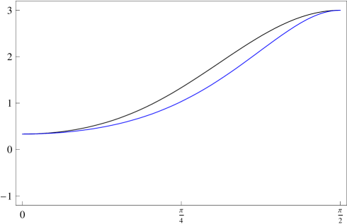
Figure 1: Plot of $m^{2}_{f\bar{f}}/M^{2}$ (upper curve) and $m_{-}^{2}/M^{2}$ (lower curve) as functions of $\theta$ for the model with quadratic Kähler potential and linear Killing vectors defined by (A.1), with $q_{1}/q_{2}=3$.

As a second simple example, let us discus the case of logarithmic Kähler potential and constant Killing vector, which corresponds to a constantly and positively curved scalar manifold with a shift isometry defined by positive shifts:

$$K=-\Lambda_{1}^{2}\log\bigg{(}\frac{\Phi^{1}+\bar{\Phi}^{1}}{\Lambda_{1}}\bigg{)}-\Lambda_{2}^{2}\log\bigg{(}\frac{\Phi^{2}+\bar{\Phi}^{2}}{\Lambda_{2}}\bigg{)}\,,\;\;X^{i}=i\,\big{(}A_{1},\,A_{2}\big{)}\,.$$ (A.10)

The two scales $\Lambda_{1}$ and $\Lambda_{2}$ define the curvatures of the two field sectors, whereas the two scales $A_{1}$ and $A_{2}$ define the gauge shifts. It is then convenient to introduce the following dimensionless parameters:

$$\lambda_{1}=\frac{g\Lambda_{1}}{M}\,,\;\;\lambda_{2}=\frac{g\Lambda_{2}}{M}\,,\;\;a_{1}=\frac{gA_{1}}{M}\,,\;\;a_{2}=\frac{gA_{2}}{M}\,.$$ (A.11)

In this case, we can parametrize the vacuum in the following way, by including absolute values to take into account that the fields are in this case restricted to have a positive real part:

$$\Phi^{i}=\text{\small$\frac{1}{\sqrt{2}}$}\,g^{\text{--}1}M\,\big{(}a_{1}\lambda_{1}|\sec\theta|,\,a_{2}\lambda_{2}|\csc\theta|\big{)}\,.$$ (A.12)

The Goldstone and Goldstino directions are then given by $x^{i}=\text{\small$\sqrt{2}$}i\,\big{(}a_{1},\,a_{2}\big{)}$ and $f^{i}=\text{\small$\sqrt{2}$}i\,\big{(}a_{1}|\tan\theta|,-a_{2}|\cot\theta|\big{)}$, whereas $g_{i\bar{\jmath}}=\frac{1}{2}\,{\rm diag}\big{(}a_{1}^{\text{--}2}\cos^{2}\theta,\,a_{2}^{\text{--}2}\sin^{2}\theta\big{)}$. The relation between $|D|$, $|F|$ and $M^{2}$ are in this case:

$$|D|=\text{\small$\frac{1}{\sqrt{2}}$}\,g^{\text{--}1}\big{(}\lambda_{1}|\cos\theta|+\lambda_{2}|\sin\theta|\big{)}\,M^{2}\,,$$ (A.13)

$$|F|=\text{\small$\frac{1}{\sqrt{2}}$}\,g^{\text{--}1}\sqrt{\lambda_{1}\lambda_{2}}\,|2\cos\theta\sin\theta|^{\text{--}1/2}\,M^{2}\,.$$ (A.14)

We then get:

$$\bigg{|}\frac{D}{F}\bigg{|}=\sqrt{|2\cos\theta\sin\theta|}\,\bigg{(}\sqrt{\frac{\lambda_{1}}{\lambda_{2}}}|\cos\theta|+\sqrt{\frac{\lambda_{2}}{\lambda_{1}}}|\sin\theta|\bigg{)}\,.$$ (A.15)

The contractions of $R_{i\bar{\jmath}k\bar{l}}$ are given by

$$R_{f\bar{f}f\bar{f}}=2g^{2}M^{\text{--}2}\big{(}\lambda_{2}^{-2}\cos^{4}\theta+\lambda_{1}^{-2}\sin^{4}\theta\big{)}\,,$$ (A.16)

$$R_{f\bar{f}x\bar{x}}=2g^{2}M^{\text{--}2}\big{(}\lambda_{2}^{-2}+\lambda_{1}^{-2}\big{)}\cos^{2}\theta\sin^{2}\theta\,,$$ (A.17)

$$R_{f\bar{f}f\bar{x}}=2g^{2}M^{\text{--}2}\big{(}\lambda_{1}^{-2}\sin^{2}\theta-\lambda_{2}^{-2}\cos^{2}\theta\big{)}|\cos\theta\sin\theta|\,.$$ (A.18)

The matrix elements of $Q_{i\bar{\jmath}}$ are instead found to be independent of the shifts $a_{i}$ and dominated by the effect of the connection term in their definition, as a result of the fact that the Killing vectors are constant:

$$Q_{f\bar{f}}=\text{\small$\sqrt{2}$}\,\big{(}\lambda_{2}^{\text{--}1}|\cos\theta|+\lambda_{1}^{\text{--}1}|\sin\theta|\big{)}|\cos\theta\sin\theta|\,,$$ (A.19)

$$Q_{x\bar{x}}=\text{\small$\sqrt{2}$}\,\big{(}\lambda_{1}^{\text{--}1}|\cos^{3}\theta|+\lambda_{2}^{\text{--}1}|\sin^{3}\theta|\big{)}\,,$$ (A.20)

$$Q_{f\bar{x}}=\text{\small$\sqrt{2}$}\,\big{(}\lambda_{1}^{\text{--}1}|\cos\theta|-\lambda_{2}^{\text{--}1}|\sin\theta|\big{)}|\cos\theta\sin\theta|\,.$$ (A.21)

The elements $m^{2}_{f\bar{f}}$, $m^{2}_{x\bar{x}}$, $m^{2}_{f\bar{x}}$ and the eigenvalues $m^{2}_{\pm}$ of the mass matrix are equal to $M^{2}$ times some functions of $\theta$ and $\lambda_{1}/\lambda_{2}$. The behavior of $m^{2}_{f\bar{f}}/M^{2}$ and $m_{-}^{2}/M^{2}$ as functions of $\theta$ is shown in fig. 2 for some particular choice of $\lambda_{1}/\lambda_{2}$. More in general, one finds the following behavior. $m^{2}_{f\bar{f}}$ reaches its maximum for $\theta=\frac{\pi}{4}$ and at that point $m^{2}_{f\bar{f}}/M^{2}=1+\frac{1}{4}(\lambda_{1}/\lambda_{2}+\lambda_{2}/\lambda_{1})$, $m^{2}_{x\bar{x}}/M^{2}=1+\frac{1}{2}(\lambda_{1}/\lambda_{2}+\lambda_{2}/\lambda_{1})$ and $m^{2}_{f\bar{x}}/M^{2}=-\frac{1}{4}(\lambda_{1}/\lambda_{2}-\lambda_{2}/\lambda_{1})$, so that $m_{-}^{2}/M^{2}$ is smaller-or-equal than $m^{2}_{f\bar{f}}/M^{2}$. The maximum of $m_{-}^{2}/M^{2}$ occurs instead for some $\theta\leq\frac{\pi}{4}$ if $\lambda_{1}>\lambda_{2}$ and for some $\theta\geq\frac{\pi}{4}$ if $\lambda_{1}<\lambda_{2}$, and takes a value that is smaller than $1+\frac{1}{4}(\lambda_{1}/\lambda_{2}+\lambda_{2}/\lambda_{1})$. For $\lambda_{1}\simeq\lambda_{2}$, the optimal direction is $\theta\simeq\frac{\pi}{4}$ and the bound is $m^{2}/M^{2}\simeq\frac{3}{2}$, which is identical to the one that one would have obtained by looking just at the Goldstino direction. For $\lambda_{1}\gg\lambda_{2}$, on the other hand, a numerical study shows that the optimal direction is $\theta\simeq 0.67$ and the bound is $m^{2}/M^{2}\simeq 0.13\,\lambda_{1}/\lambda_{2}$, which is a factor $1.86$ smaller than the one that one would have inferred by looking just at the Goldstino direction, although still positive. For $\lambda_{1}\ll\lambda_{2}$, the situation is similar but with $\lambda_{1}\leftrightarrow\lambda_{2}$ and $\theta\leftrightarrow\frac{\pi}{2}-\theta$.

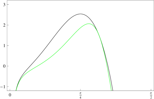
Figure 2: Plot of $m^{2}_{f\bar{f}}/M^{2}$ (upper curve) and $m_{-}^{2}/M^{2}$ (lower curve) as functions of $\theta$ for the model with logarithmic Kähler potential and constant Killing vectors defined by (A.10), with $\lambda_{1}/\lambda_{2}=\frac{1}{6}$.

As a third slightly more complicated and richer example, let us finally discus the case of logarithmic Kähler potential and linear Killing vector, which corresponds to a constantly and positively curved scalar manifold with a phase isometry defined by positive charges:

$$K=-\Lambda_{1}^{2}\log\bigg{(}1-\frac{\!\Phi^{1}\bar{\Phi}^{1}\!}{\Lambda_{1}^{2}}\hskip 1.0pt\bigg{)}-\Lambda_{2}^{2}\log\bigg{(}1-\frac{\!\Phi^{2}\bar{\Phi}^{2}\!}{\Lambda_{2}^{2}}\hskip 1.0pt\bigg{)}\,,\;\;X^{i}=-i\,\big{(}q_{1}\Phi^{1},q_{2}\Phi^{2}\big{)}\,.$$ (A.22)

The two scales $\Lambda_{1}$ and $\Lambda_{2}$ define as before the curvatures of the two field sectors. It turns out that by varying the overall scale of these curvatures with respect to the vector mass scale, this new model interpolates between the two previous ones. This can be seen as follows. The small curvature limit corresponds to take $\Lambda_{i}$ large and $\Phi^{i}$ finite, so that $\Phi^{i}/\Lambda_{i}$ is close to $0$. In this limit one can keep the same coordinates and just expand the logarithm in $K$. In this way one then recovers the model (A.1). The large curvature limit corresponds instead to take $\Lambda_{i}$ small and $\Phi^{i}$ also small, so that $\Phi^{i}/\Lambda_{i}$ is close to $1$. In this limit, it is convenient to change coordinates to describe the model in a more transparent way. The appropriate reparametrization turns out to be $\Phi^{i}/\Lambda_{i}\to(1-\frac{1}{2}\Phi^{i}/\Lambda_{i})/(1+\frac{1}{2}\Phi^{i}/\Lambda_{i})$. Discarding an irrelevant Kähler transformation, one then finds $K\to-\sum_{i}\Lambda_{i}^{2}\log((\Phi^{i}+\bar{\Phi}^{i})/\Lambda_{i})$ and $X^{i}\to i\,q_{i}\Lambda_{i}\,(1-\frac{1}{4}\Phi^{i2}/\Lambda_{i}^{2})$. In these new coordinates, $\Phi^{i}/\Lambda_{i}$ is close to $0$. In this limit one then manifestly recovers the model (A.10) with the same field parametrization and shifts given by $A_{i}=q_{i}\Lambda_{i}$. To parametrize the effects of the curvatures, we introduce as before the dimensionless parameters

$$\lambda_{1}=\frac{g\Lambda_{1}}{M}\,,\;\;\lambda_{2}=\frac{g\Lambda_{2}}{M}\,.$$ (A.23)

It will also be useful to introduce the short-hand notation

$$u(\theta)=H\bigg{(}\frac{\cos\theta}{q_{1}\lambda_{1}}\bigg{)}\,,\;\;v(\theta)=H\bigg{(}\frac{\sin\theta}{q_{2}\lambda_{2}}\bigg{)}\,.$$ (A.24)

where $H(x)$ is the following monotonically decreasing function:

$$H(x)=\frac{\sqrt{1+2\,x^{2}}-1}{x^{2}}\simeq\Bigg{\{}\begin{array}[]{l}\!1\;\;\;\;\;\;\;,\;\;|x|\ll 1\\[4.2679pt] \!\text{\small$\sqrt{2}$}/|x|\,,\;\;|x|\gg 1\\ \end{array}\,.$$ (A.27)

In this case, we can parametrize the vacuum in the following way:

$$\Phi^{i}=\text{\small$\frac{1}{\sqrt{2}}$}\,g^{\text{--}1}M\,\big{(}q_{1}^{\text{--}1}u(\theta)\cos\theta,\,q_{2}^{\text{--}1}v(\theta)\sin\theta\big{)}\,.$$ (A.28)

The Goldstone and Goldstino directions then read $x^{i}=-i\,\big{(}u(\theta)\cos\theta,\,v(\theta)\sin\theta\big{)}$ and $f^{i}=-i\,\big{(}u(\theta)\sin\theta,-v(\theta)\cos\theta\big{)}$, and the metric is $g_{i\bar{\jmath}}={\rm diag}\big{(}1/u^{2}(\theta),\,1/v^{2}(\theta)\big{)}$. The relation between $|D|$, $|F|$ and $M^{2}$ are in this case:

$$|D|=\text{\small$\frac{1}{2}$}g^{\text{--}1}\,\big{(}q_{1}^{\text{--}1}u(\theta)\cos^{2}\theta+q_{2}^{\text{--}1}v(\theta)\sin^{2}\theta\big{)}M^{2}\,,$$ (A.29)

$$|F|=\text{\small$\frac{1}{2}$}g^{\text{--}1}\sqrt{\frac{q_{1}^{\text{--}1}u(\theta)\cos^{2}\theta+q_{2}^{\text{--}1}v(\theta)\sin^{2}\theta}{q_{2}\big{[}2/v(\theta)-1\big{]}\cos^{2}\theta+q_{1}\big{[}2/u(\theta)-1\big{]}\sin^{2}\theta}}\,M^{2}\,.$$ (A.30)

We then get:

$$\bigg{|}\frac{D}{F}\bigg{|}=\sqrt{\sqrt{\frac{q_{2}}{q_{1}}}u(\theta)\cos^{2}\theta+\sqrt{\frac{q_{1}}{q_{2}}}v(\theta)\sin^{2}\theta}$$

$$\hskip 35.0pt\times\sqrt{\sqrt{\frac{q_{2}}{q_{1}}}\big{[}2/v(\theta)-1\big{]}\cos^{2}\theta+\sqrt{\frac{q_{1}}{q_{2}}}\big{[}2/u(\theta)-1\big{]}\sin^{2}\theta}\,.$$ (A.31)

The contractions of $R_{i\bar{\jmath}k\bar{l}}$ are given by

$$R_{f\bar{f}f\bar{f}}=2g^{2}M^{\text{--}2}\big{(}\lambda_{2}^{-2}\cos^{4}\theta+\lambda_{1}^{-2}\sin^{4}\theta\big{)}\,,$$ (A.32)

$$R_{f\bar{f}x\bar{x}}=2g^{2}M^{\text{--}2}\big{(}\lambda_{2}^{-2}+\lambda_{1}^{-2}\big{)}\cos^{2}\theta\sin^{2}\theta\,,$$ (A.33)

$$R_{f\bar{f}f\bar{x}}=2g^{2}M^{\text{--}2}\big{(}\lambda_{1}^{-2}\sin^{2}\theta-\lambda_{2}^{-2}\cos^{2}\theta\big{)}\cos\theta\sin\theta\,.$$ (A.34)

The matrix elements of $Q_{i\bar{\jmath}}$ are instead found to be:

$$Q_{f\bar{f}}=q_{2}\big{[}2/v(\theta)-1\big{]}\cos^{2}\theta+q_{1}\big{[}2/u(\theta)-1\big{]}\sin^{2}\theta\,,$$ (A.35)

$$Q_{x\bar{x}}=q_{1}\big{[}2/u(\theta)-1\big{]}\cos^{2}\theta+q_{2}\big{[}2/v(\theta)-1\big{]}\sin^{2}\theta\,,$$ (A.36)

$$Q_{f\bar{x}}=\big{(}q_{1}\big{[}2/u(\theta)-1\big{]}-q_{2}\big{[}2/v(\theta)-1\big{]}\big{)}\cos\theta\sin\theta\,.$$ (A.37)

The elements $m^{2}_{f\bar{f}}$, $m^{2}_{x\bar{x}}$, $m^{2}_{f\bar{x}}$ and the eigenvalues $m^{2}_{\pm}$ of the mass matrix are equal to $M^{2}$ times some functions of $\theta$, $\lambda_{1}/\lambda_{2}$, $q_{1}/q_{2}$ and $q_{1}q_{2}\lambda_{1}\lambda_{2}$. The behavior of $m^{2}_{f\bar{f}}/M^{2}$ and $m_{-}^{2}/M^{2}$ as functions of $\theta$ is shown in fig. 3 for some particular choice of $\lambda_{1}/\lambda_{2}$, $q_{1}/q_{2}$ and $q_{1}q_{2}\lambda_{1}\lambda_{2}$. More in general, one finds the following behavior. $m^{2}_{f\bar{f}}$ and $m_{-}^{2}$ reach maxima for two different values of $\theta$, and the maximal value of $m_{-}^{2}$ is always smaller than the maximal value of $m^{2}_{f\bar{f}}$. This shows once again that the bound that one would have inferred by looking only at the Goldstino direction is weaker than the bound $m^{2}$ that one obtains by taking into account also the Goldstone direction. One moreover verifies that in the limit $\lambda_{i}\gg 1$ one recovers the behavior of the model with quadratic $K$ and linear $X^{i}$ with charges $q_{i}$, whereas in the limit $\lambda_{i}\ll 1$ one reaches the behavior of the model with logarithmic $K$ and constant $X^{i}$ with shifts $A_{i}=q_{i}\Lambda_{i}$.

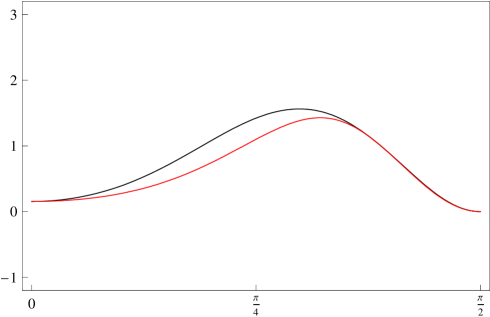
Figure 3: Plot of $m^{2}_{f\bar{f}}/M^{2}$ (upper curve) and $m_{-}^{2}/M^{2}$ (lower curve) as functions of $\theta$ for the model with logarithmic Kähler potential and linear Killing vectors defined by (A.22), with $\lambda_{1}/\lambda_{2}=\frac{1}{6}$, $q_{1}/q_{2}=3$ and $q_{1}q_{2}\lambda_{1}\lambda_{2}=1$.

References

• [1] S. Ferrara, L. Girardello and F. Palumbo, A general mass formula in broken supersymmetry, Phys. Rev.  D 20, 403 (1979).
• [2] M. T. Grisaru, M. Rocek and A. Karlhede, The superHiggs effect in superspace, Phys. Lett.  B 120, 110 (1983).
• [3] C. M. Hull, A. Karlhede, U. Lindstrom and M. Rocek, Nonlinear sigma models and their gauging in and out of superspace, Nucl. Phys.  B 266 (1986) 1.
• [4] S. Ray, Some properties of meta-stable supersymmetry-breaking vacua in Wess-Zumino models, Phys. Lett.  B 642 (2006) 137 [arXiv:hep-th/0607172].
• [5] Z. Komargodski and D. Shih, Notes on SUSY and R-Symmetry breaking in Wess-Zumino models, JHEP 0904 (2009) 093 [arXiv:0902.0030 [hep-th]].
• [6] M. Gómez-Reino and C. A. Scrucca, Locally stable non-supersymmetric Minkowski vacua in supergravity, JHEP 0605 (2006) 015 [hep-th/0602246].
• [7] M. Gómez-Reino and C. A. Scrucca, Constraints for the existence of flat and stable non-supersymmetric vacua in supergravity, JHEP 0609 (2006) 008 [hep-th/0606273].
• [8] F. Denef and M. R. Douglas, Distributions of nonsupersymmetric flux vacua, JHEP 0503 (2005) 061 [arXiv:hep-th/0411183].
• [9] L. Covi, M. Gómez-Reino, C. Gross, J. Louis, G. A. Palma and C. A. Scrucca, De Sitter vacua in no-scale supergravities and Calabi-Yau string models, JHEP 0806 (2008) 057 [arXiv:0804.1073 [hep-th]].
• [10] L. Covi, M. Gómez-Reino, C. Gross, G. A. Palma and C. A. Scrucca, Constructing de Sitter vacua in no-scale string models without uplifting, JHEP 0903 (2009) 146 [arXiv:0812.3864 [hep-th]].
• [11] T. Gregoire, R. Rattazzi and C. A. Scrucca, D-type supersymmetry breaking and brane-to-brane gravity mediation, Phys. Lett.  B 624 (2005) 260 [arXiv:hep-ph/0505126].
• [12] K. R. Dienes, B. Thomas, Building a nest at tree level: classical metastability and non-trivial vacuum structure in supersymmetric field theories, Phys. Rev.  D78 (2008) 106011. [arXiv:0806.3364 [hep-th]].
• [13] L. F. Matos, Some examples of F and D-term SUSY breaking models, arXiv:0910.0451 [hep-ph].
• [14] M. Gómez-Reino and C. A. Scrucca, Metastable supergravity vacua with F and D supersymmetry breaking, JHEP 0708 (2007) 091 [arXiv:0706.2785 [hep-th]].
• [15] M. Gomez-Reino, J. Louis and C. A. Scrucca, No metastable de Sitter vacua in N=2 supergravity with only hypermultiplets, JHEP 0902 (2009) 003 [arXiv:0812.0884 [hep-th]].
• [16] E. Cremmer, C. Kounnas, A. Van Proeyen, J. P. Derendinger, S. Ferrara, B. de Wit and L. Girardello, Vector multiplets coupled to N=2 supergravity: superHiggs effect, flat potentials and geometric structure, Nucl. Phys.  B 250 (1985) 385.
• [17] J.-C. Jacot and C. A. Scrucca, Metastable supersymmetry breaking in N=2 non-linear sigma-models, Nucl. Phys.  B 840 (2010) 67 [arXiv:1005.2523 [hep-th]].
• [18] P. Frè, M. Trigiante and A. Van Proeyen, Stable de Sitter vacua from N = 2 supergravity, Class. Quant. Grav.  19 (2002) 4167 [arXiv:hep-th/0205119].
• [19] O. Ogetbil, Stable de Sitter vacua in 4 dimensional supergravity originating from 5 dimensions, Phys. Rev.  D 78 (2008) 105001 [arXiv:0809.0544 [hep-th]].
• [20] D. Roest and J. Rosseel, De Sitter in extended supergravity, Phys. Lett.  B 685 (2010) 201 [arXiv:0912.4440 [hep-th]].
• [21] I. Antoniadis and M. Buican, Goldstinos, supercurrents and metastable SUSY breaking in N=2 supersymmetric gauge theories, JHEP 1104 (2011) 101 [arXiv:1005.3012 [hep-th]].
• [22] T. T. Dumitrescu, Z. Komargodski and M. Sudano, Global symmetries and D-terms in supersymmetric field theories, JHEP 1011 (2010) 052 [arXiv:1007.5352 [hep-th]].
• [23] L. Brizi and C. A. Scrucca, Effects of heavy modes on vacuum stability in supersymmetric theories, JHEP 1011 (2010) 134 [arXiv:1009.0668 [hep-th]].
• [24] N. Arkani-Hamed, S. Dimopoulos, G. F. Giudice and A. Romanino, Aspects of split supersymmetry, Nucl. Phys.  B 709 (2005) 3 [arXiv:hep-ph/0409232].
• [25] M. Nardecchia, A. Romanino and R. Ziegler, General aspects of tree level gauge mediation, JHEP 1003 (2010) 024 [arXiv:0912.5482 [hep-ph]].
• [26] Y. Kawamura, Limitation on magnitude of D-components, Prog. Theor. Phys.  125 (2011) 509 [arXiv:1008.5223 [hep-ph]].