On ringing effects near jump discontinuities

for periodic solutions to dispersive partial

differential equations

B Y K ENNETH D. T.-R. M C L AUGHLIN ^1,2 AND N IGEL J. E. P ITT ^2,3, ​​

¹Department of Mathematics, University of Arizona, Tucson, AZ 85721, USA

²Departamento de Matemática, Universidade de Brasília, DF 70910-900, Brazil

³School of Mathematics, Institute for Advanced Study, Princeton, NJ 08540, USA

We consider weak solutions to dispersive partial differential equations with periodic boundary conditions and initial data with jump discontinuities. These are already known to be continuous at irrational times and piecewise constant at rational times; we show that as time approaches a rational value the solution exhibits a ringing effect, with the characteristic overshoot of fixed amplitude near the discontinuities. Furthermore this effect is the same whether the sequence of times follows rational or irrational values.

Keywords: ringing effect; dispersive equations; weak solutions, periodic boundary conditions;

Diophantine approximations; Weyl shift method

 

1. Introduction

Consider the equation

$$U^{(0,n)}(t,x)=(2\pi i)^{n-1}U^{(1,0)}(t,x)$$ (1.1)

for $n\geq 2$. Any classical solution to this equation satisfies the condition that

$$\mathop{\vtop{\halign{#\cr$\hfil\displaystyle{\int{\hskip-5.69054pt}\int}\hfil$\crcr\kern 1.0pt\nointerlineskip\cr\kern-2.0pt\cr}}}\limits_{{\mathbb{R}}^{2}}U(t,x)\left\{F^{(0,n)}(t,x)-(-2\pi i)^{n-1}F^{(1,0)}(t,x)\right\}dx\,dt=0$$ (1.2)

for any ${\hbox{\script C}}^{\,\,\infty}$ function $F$ of compact support in ${\mathbb{R}}^{2}$, as can be seen using integration by parts, and we call a function $U(t,x)$ satisfying $(1.2)$ a weak solution to $(1.1)$. We are interested here in weak solutions with periodic boundary conditions $U(t,x+1)=U(t,x)$ for all $x$. It is natural to study such solutions through their representations by Fourier series, which are of course ubiquitous in mathematics, and we will use techniques from analytic number theory to analyse these series and show some asymptotic properties of the weak solution $U(t,x)$.

To motivate this, for the present consider the simpler case of $(1.1)$ for $n=2$ with vanishing boundary conditions $U(t,x)\rightarrow 0$ as $x\rightarrow\pm\infty$, and initial data with jump discontinuities; for instance $U(0,x)=\chi(x)$, where $\chi$ is the characteristic function of the interval $[-\gamma,\gamma]$ for $0<\gamma<1/2$. By considering the Fourier transform in $x$ of $U(t,x)$ one can show that

$$U(t,x)=\int\limits_{-\infty}^{\infty}{\hat{U}}(0,k)e(tk^{2}+xk)dk=\int\limits_{-\infty}^{\infty}\frac{\sin 2\pi\gamma k}{\pi k}e(tk^{2}+xk)dk$$ (1.3)

where we have used the notational convention $e(\xi)=e^{2\pi i\xi}$, as throughout this paper. With $t=0$, the integral represents the initial data $\chi(x)$ in $L^{2}$. Moreover it is not hard to prove that the truncated integral

$$U(0,x;N):=\int_{-N}^{N}\frac{\sin{2\pi\gamma k}}{\pi k}e\left(xk\right)dk$$

converges pointwise to $\chi(x)$. Of course, the convergence cannot be uniform and indeed one has

$$\lim_{N\to\infty}U\left(0,\gamma+s/N;N\right)=\frac{1}{2}-\frac{1}{\pi}\int_{0}^{s}\frac{\sin{2\pi w}}{w}dw.$$

This is the well-known Gibbs phenomenon, which is an oscillatory ringing produced by truncation of the Fourier representation of a function with a discontinuity.

There is, however, an entirely different phenomenon, which is an oscillatory ringing produced not by truncation but rather by a different mechanism which, as we will explain, should be thought of as a dispersive regularization of a discontinuity. Indeed, by contour deformation or otherwise, the integral solution (1.3) can be seen to be analytic in $t$ or $x$ if $t>0$. Away from $x=\pm\gamma$ the integral converges nicely to $U(0,x)$ as $t\rightarrow 0^{+}$, however in the rescaled variable $s$ where $x=\pm\gamma+st^{1/2}$ one can obtain the asymptotic expression (see DiFranco & McLaughlin 2005)

$$U\left(t,\gamma+st^{1/2}\right)=\frac{1}{2}-\frac{1}{2}\,{\hbox{\rm Erf}}\,\left({\sqrt{\frac{\pi}{2}}}e^{-i\pi/4}s\right)+O\left(t^{1/2}\right)$$ (1.4)

where Erf denotes the usual error function (see Abramovitz & Stegun 1972). Similar phenomena can be shown to occur for $n>2$, although with different ringing functions.

Our goal here is to study similar effects in the more complicated situation where $U(t,x)$ obeys periodic boundary conditions, which have not been observed previously, and to give asymptotic expressions for these effects. Here Fourier series expansions replace the Fourier transform (or if one prefers, series replace integrals), and the resulting structure is more complicated, presenting ringing effects at all rational times, not just at zero as in the “whole line” case. The general setup is as follows. Suppose now that $U(t,x)$ is defined on $[0,\delta]\times{\mathbb{R}}$ for some $\delta>0$ and is periodic in $x$, that is, $U(t,x)=U(t,x+1)$ for all $t$ and $x$. Such a function has a Fourier series

$$U(t,x)\sim\sum_{k=-\infty}^{\infty}c_{k}(t)e(kx)\ ,\ c_{k}(t)=\int\limits_{0}^{1}U(t,\xi)e(-k\xi)d\xi.$$ (1.5)

If $U(t,x)$ is a square-integrable weak solution to $(1.1)$ then standard arguments show that $c_{k}(t)=c_{k}e(tk^{n})$ where the constants $c_{k}$ are the Fourier coefficients of $U(0,x)$, and where the convergence of the series to $U(t,x)$ is understood in the $L^{2}$ sense. Note that periodicity in $x$ has forced periodicity in $t$ also, which is the root cause of the special behaviour at rational times. We will say a function $f(x)$ is in class D if it is integrable, periodic of period 1, piecewise continuously differentiable, and $f(x)=\left\{f\left(x^{+}\right)+f\left(x^{-}\right)\right\}/2$ for all $x$. It is a well-known theorem of harmonic analysis (see Katznelson 2004, for instance) that functions $f$ of class D have Fourier series that converge pointwise to $f$, in the sense that

$$f(x)=\lim_{K\rightarrow\infty}\sum_{|k|\leq K}c_{k}e(kx)\ ,$$

that is, the series converges pointwise once written in terms of sines and cosines rather than exponentials. (The series of exponentials may diverge, in the literal sense). We will consider periodic discontinuous initial conditions

$$U(0,x)=\sum_{l=-\infty}^{\infty}\chi_{[-\gamma,\gamma]}(x+l)$$ (1.6)

where $0<\gamma<1/2$, which is in class D, with $c_{k}=(\pi k)^{-1}\sin 2\pi\gamma k$, so the Fourier series $(1.5)$ for $U(t,x)$ is

$$U(t,x)\sim\sum_{k}\frac{\sin 2\pi\gamma k}{\pi k}e(tk^{n}+xk)\ .$$ (1.7)

The series clearly converges in the $L^{2}$ sense, and represents the unique weak solution in that space. We will show some structural properties of $U(t,x)$ by identifiying it with this series representation and considering the properties of the series.

To understand why the situation should be so much more complicated requires reviewing some known results. In a variety of applied sciences, the term “dispersive” describes a localized quantity which spreads out as time passes. In the context of wave phenomena, an equation is called dispersive if its simple oscillatory solutions propagate at velocities that depend on their spatial frequencies. This is the case here; rewriting the coefficients as $e(k(x+k^{n-1}t))$ they can be seen as a family of traveling waves with velocity $k^{n-1}$, which is clearly dependent on the spatial frequency $k$. Thus if one starts with localised initial data the various terms of the Fourier series of the solution spread out in space, since they move at different velocities. As time passes the solution will appear more extended, with the highest spatial frequency components most apparent in the furthest reaches of the solution. Properly speaking, dispersion requires sufficient extent to permit the observation of spreading. This may, or may not, be the case for a partial differential equation with periodic boundary conditions, but nonetheless such an equation is still called dispersive if its family of solutions have frequency dependent velocity. In this context it is striking that periodic boundary conditions should cause a dispersive equation like (1.1) to show recurrence, as well as radically different behaviour at rational and irrational times. This can be seen experimentally in the case $n=2$, as reported by Talbot 1836, who shone light on a periodic grating and looked at the images produced by it. He reports “…a regular alternation of numerous lines or bands of red and green colour, having their direction parallel to the lines of the grating. On removing the lens a little further from the grating, the bands gradually changed their colours, and became alternately blue and yellow.” (Talbot 1836). This is now known as the Talbot effect, and has been extensively studied; we refer the reader to Berry & Klein 1996 for details of the effect, but also for two contributions which are pertinent to our discussion here. Supposing that the period of the grating is $a$ and that the wavelength of the light is $\lambda$, the images seen by Talbot form at regular multiples of $a^{2}/\lambda$. (In the context of $(1.1)$, we can view Talbot’s grating as initial data which is periodic, being $1$ on the slits of the grating and zero elsewhere). Berry and Klein observe that at rational multiples $(p/q)a^{2}/\lambda$ of this distance “…these fractional Talbot images consist of $q$ equally spaced copies of the transmission function of the grating, which superpose coherently when they add up.”. Furthermore, they show that these translates have phases given by Gauss sums, so the solutions can be written down explicitly at rational times, and are piecewise constant functions of $x$. (This was also discussed in Olver 2010). They also observe that this is in sharp contrast with irrational times; considering the solution at a sequence of rational times tending to an irrational $t$, they show that “the graph of a function with power spectrum $|g_{n}|^{2}$ proportional to $n^{-\beta}$ is a fractal curve with fractal dimension $D=(5-\beta)/2$. A smooth curve has $D=1$, and a curve with $D=2$ is so jagged that it is almost area filling; curves with $1<D<2$ are continuous but non-differentiable. Thus, since the fourier coefficients of the initial data have power spectrum decaying like $n^{-2}$, the fractal dimension must be $3/2$.”

A number of researchers from a variety of different areas of analysis, including Arkhipov & Oskolkov 1989, Stein & Wainger 1990, Oskolkov 1992, Kapitanski & Rodnianski 1999, Rodnianski 1999 and Rodnianski 2000, put these ideas on a rigorous footing by establishing convergence properties of the associated Fourier series in the space of continuous functions. One result which is particularly pertinent to the discussion here is due to Rodnianski 2000: this discusses periodic solutions to $(1.1)$ with $n=2$ with initial data of bounded variation but not in the space $\cup_{\epsilon>0}H^{1/2+\varepsilon}$. (Here the Sobolev space $H^{s}$ is the space of functions whose Fourier coefficients $\hat{f}(k)$ satisfy $\sum_{k=1}^{\infty}|\hat{f}(k)|^{2}(1+|k|^{2})^{s/2}\ <\infty$.) The result states that for almost all irrational $t$, including all algebraic $t$, the fractal dimension of the graphs of the real and imaginary parts of $U(t,x)$ (which are continuous functions of $x$) is 3/2.

In fact there is a dichotomy between rational and irrational times for all $n\geq 2$, which is reflected in our calculations. In contrast to the considerations in Berry & Klein 1996 or Rodnianski 2000, which consider sequences of rational times tending to an irrational limit, to understand the nature of the function at irrational times, we consider sequences of times, rational or irrational, tending to a rational limit, to understand the ringing phenomena exhibited.

As observed above $(1.7)$ converges in $L^{2}$ to $U(t,x)$, however convergence in any stronger sense is more complicated, depending greatly for the reasons mentioned above on whether $t$ is rational or irrational. For irrational times $t$ we will use rational approximations; we speak of approximants as being reduced fractions $u/q$ such that

$$\left|t-\frac{u}{q}\right|<\frac{1}{q^{2}}\ .$$ (1.8)

There are infinitely many approximants to any irrational $t$, some of them given by the convergents $u_{j}/q_{j}\in{\mathbb{Q}}$ from the continued fraction expansion to $t$, which obey the inequality

$$\left|t-\frac{u_{j}}{q_{j}}\right|<\frac{1}{q_{j}q_{j+1}}\ .$$ (1.9)

(See Hua 1982 or Hardy & Wright 1979). Note also that a celebrated theorem in Roth 1955 states that if $t$ is an algebraic irrational then for any $\eta>0$ there are only finitely many solutions to

$$\left|t-\frac{u}{q}\right|<\frac{1}{q^{2+\eta}}.$$ (1.10)

We need to introduce some sets of irrationals described by their rational approximations. To this end $n\geq 2$ will always represent the order of the equation $(1.1)$, and $\Delta$ will be fixed once and for all in $(0,1)$, and in $(0,1/2)$ in the case $n=2$. Note that several of the sets and implied constants below will depend on $n$ and $\Delta$ without this being explicitly mentioned or shown in the notation.

Definition 1.1. Define A to be the set of $t\in[0,1]$ such that for all sufficiently large $M$ there is an approximant $u/q$ to $t$ with

$$M^{\Delta}<q\leq M^{n-\Delta}$$ (1.11)

and define ${\hbox{\script A}}_{m}$ to be the set of $t\in[0,1]$ such that for all $M\geq m$ there is an approximant $u/q$ to $t$ satisfying $(1.11)$. Further, for $\alpha>0$ define ${\hbox{\script B}}_{m,\alpha}$ to be the set of $t\in[0,1]$ such that for all $M\geq mt^{-\alpha}$ there is an approximant $u/q$ to $t$ satisfying $(1.11)$.

Although some parts are not strictly necessary below, we prove the following lemma.

Lemma 1.2. Let $\mu$ denote Lebesgue measure, and suppose $(n-\Delta)^{-1}<\alpha<\Delta^{-1}$.

1. If $m_{1}\leq m_{2}$ then ${\hbox{\script A}}_{m_{1}}\subseteq{\hbox{\script A}}_{m_{2}}$.

2. If $t\in{\hbox{\script A}}$ then there exists $m$ such that $t\in{\hbox{\script A}}_{m}$, so ${\hbox{\script A}}=\bigcup_{m\geq 2}{\hbox{\script A}}_{m}$.

3. There is a constant $c_{n,\Delta}$ such that $\mu\left({\hbox{\script A}}_{m}\right)\geq 1-c_{n,\Delta}m^{1+2\Delta-n}$, which tends to $1$ as $m\rightarrow\infty$, so $\mu\left({\hbox{\script A}}\right)=1$.

4. A contains all algebraic irrationals.

5. For all $m$, ${\hbox{\script A}}_{m}\subseteq{\hbox{\script B}}_{m,\alpha}$, so $\mu\left({\hbox{\script B}}_{m,\alpha}\right)\rightarrow 1$ as $m\rightarrow\infty$.

6. There is a constant $c_{n,\Delta,\alpha}$ such that

$$\mu\left({\hbox{\script B}}_{m,\alpha}\cap[0,t_{0}]\right)\geq t_{0}\left(1-c_{n,\Delta,\alpha}t_{0}^{(n-1-2\Delta)\alpha}m^{-n+\Delta+1}\right).$$

The convergence of the series $(1.7)$ is described in the following result.

Theorem 1.3. Let

$$S_{K}=\sum_{0<|k|\leq K}\frac{e(tk^{n}+xk)}{k}\ .$$ (1.12)

1. If $t$ is rational then $S_{K}$ converges pointwise in $x$ to a piecewise constant function.

2. If $t\in{\hbox{\script A}}$ then the sequence $S_{K}$ converges uniformly in $x$.

Note that Arkhipov and Oskolkov 1989 have shown that a more general class of series converges pointwise, and hence the partial sums $(1.12)$ converge pointwise in $x$ for all times. Their proof uses Vinogradov’s method for exponential sums in place of the Weyl shift method described below and used here; we state and prove Theorem 1.3 since it is necessary to Theorem 1.5 below, for which we are as yet unable to apply the Vinogradov method.

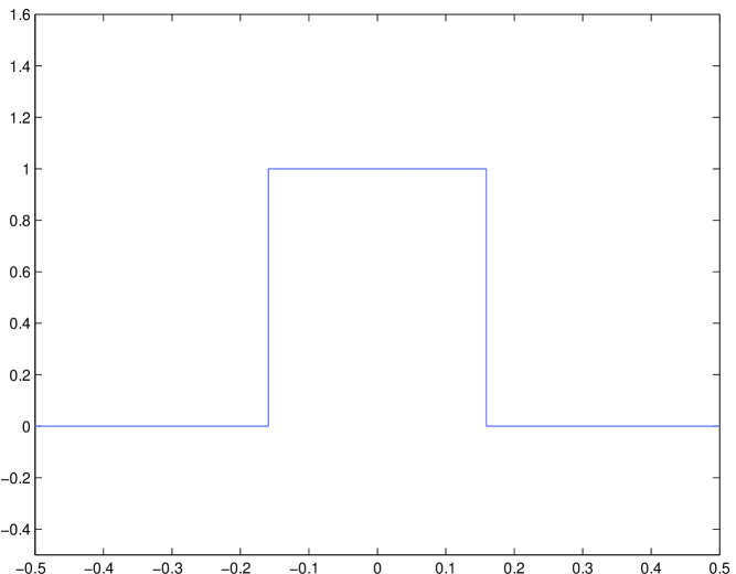
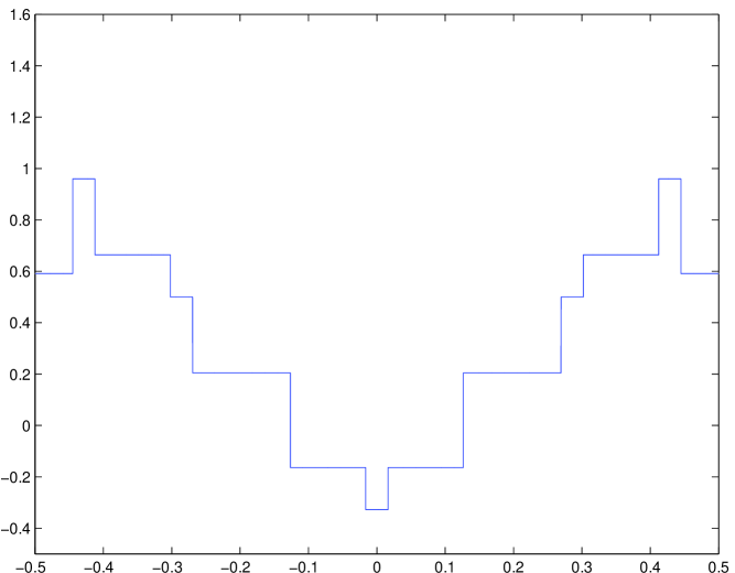
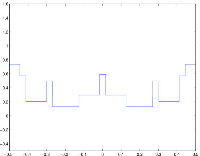
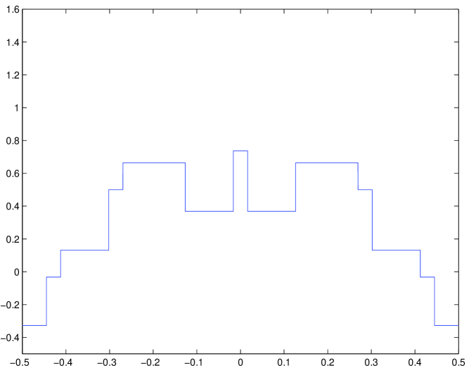
Figure 1: The real part of $U(t,x)$ for $n=2$ at $u/7$ for $u=0,1,2,3$ and $u=4,5,6,7$

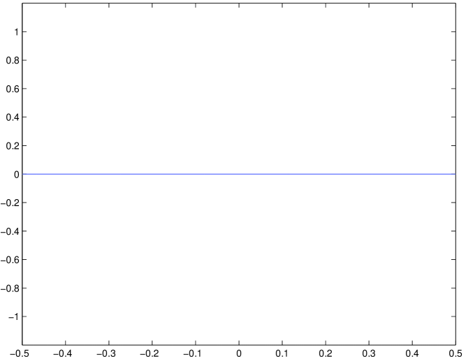
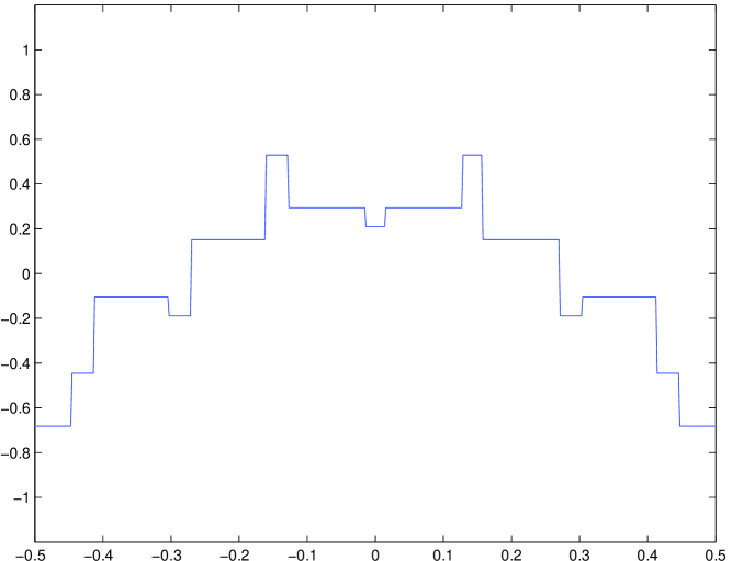
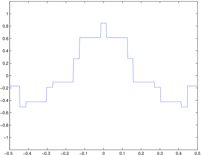
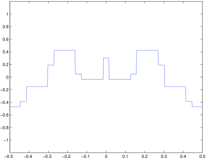
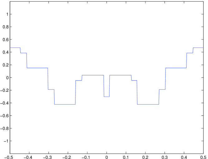
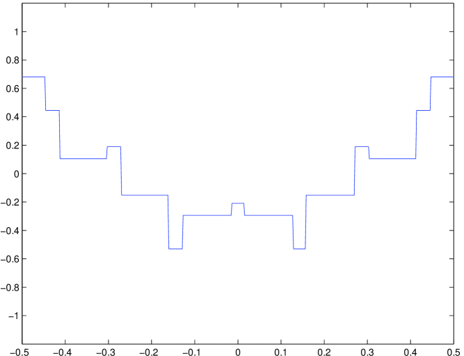
Figure 2: The imaginary part of $U(t,x)$ for $n=2$ at $u/7$ for $u=0,1,2,3$ and $u=4,5,6,7$

As discussed above, Part 1 of this Theorem has been noted elsewhere. The same result is true, however, in a much more general context than we can prove Part 2, so we state and prove it separately, and deduce 1 of Theorem 1 as an immediate corollary.

Theorem 1.4. Let $P$ be a polynomial with integer coefficients and $L$ be the differential operator

$$L=2\pi iP\left(\frac{1}{2\pi i}\frac{\partial}{\partial x}\right),$$

and consider the initial value problem

$$LU(t,x)=U_{t}(t,x)$$ (1.13)

with $U(0,x)=f(x)$, where $f\in{\hbox{\script D}}$ and $f(x+1)=f(x)$. Denoting

$$G(u,v;q)=\sum_{w({\hbox{\smallrm mod}}\ q)}e_{q}(uP(w)-vw),$$ (1.14)

at the rational time $t=u/q$ we have

$$U(t,x)=\frac{1}{q}\sum_{v({\hbox{\smallrm mod}}\,q)}G(u,v;q)f\left(x+\frac{v}{q}\right)\ .$$ (1.15)

Thus if $U(0,x)$ is piecewise constant, $U(t,x)$ is piecewise constant at all rational times.

We can rephrase this theorem as saying that at rational times $t$ the solution to the initial value problem $(1.13)$ is a linear combination of translates of the initial data. Note also that very generally (see Schmidt 2004) we have $G\ll q^{1/2+\varepsilon}$, a bound which is not necessary to prove Theorem 2, but which we will use elsewhere; in particular note that

$$\sum_{w({\hbox{\smallrm mod}}\,q)}e_{q}\left({{uw^{n}-vw}}\right)\ll(u,v,q)^{1/2}q^{1/2+\varepsilon}$$ (1.16)

where $(u,v,q)$ denotes the greatest common divisor of $u,v$ and $q$, and where the implied constant depends on $\varepsilon$ and $n$. As noted in Berry & Klein 1996, in the special case of the Schrödinger equation these sums are Gauss sums and can be evaluated for general $q$, but in general this is not realistic and we must be satisfied with estimates. We omit the proof of $(1.16)$, merely noting that it follows from Theorem 2.5 in Schmidt 2004, which contains an extensive discussion of these issues.

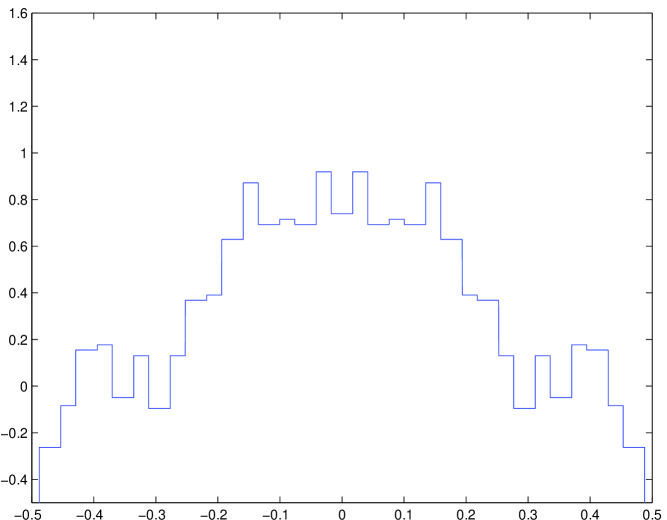
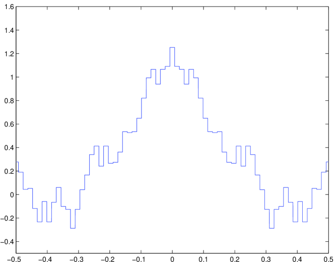
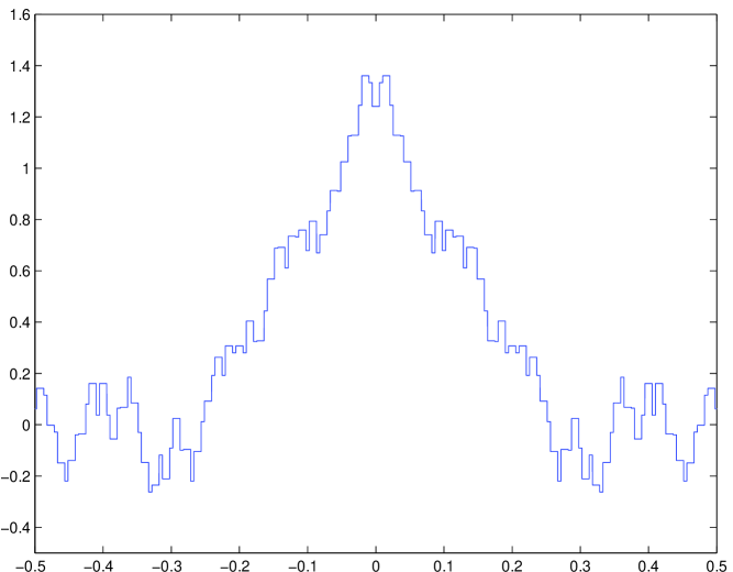
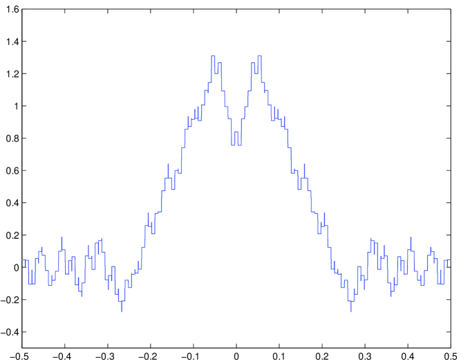
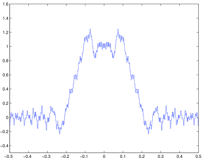
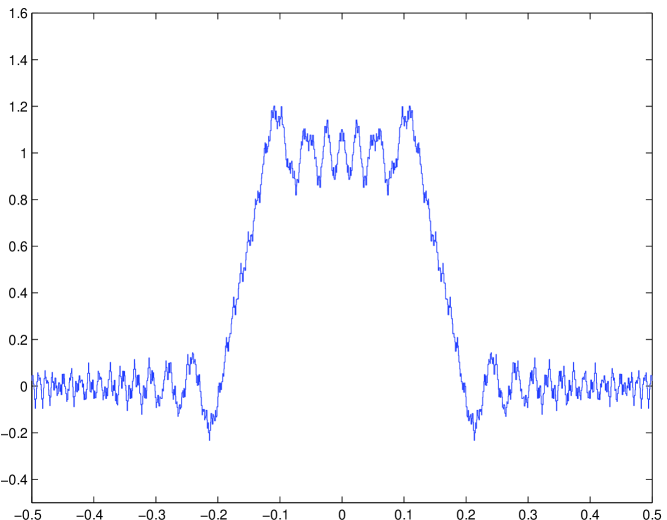
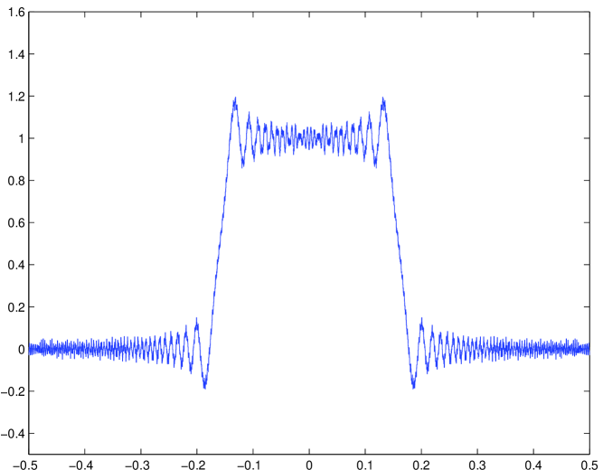
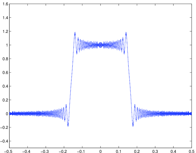
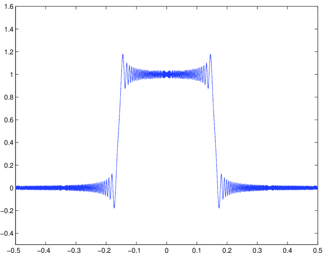
Figure 3: $U(t,x)$ for $n=2$ and $u/q=1/17,1/33,1/65$, $1/129.1/257,1/513$, and $1/2049,1/4097,1/7374$

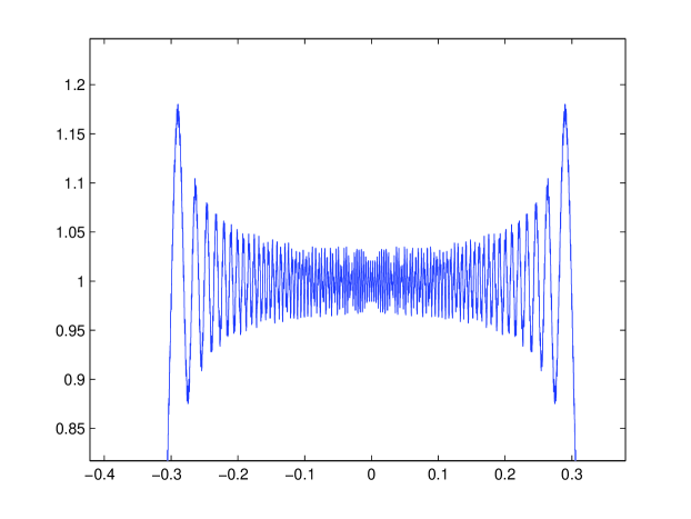
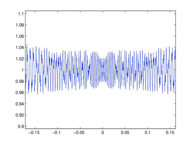
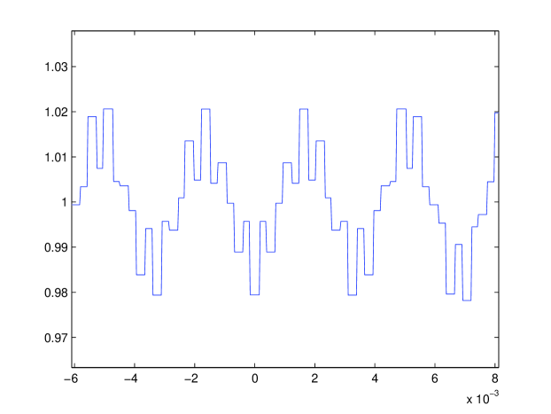
Figure 4: Zoomed-in sections from $U(t,x)$ for $n=2$ and $u/q=1/7374$

An example is given by the solution to $(1.1)$ in the case $n=2$ and $\gamma=1/\pi$, at the rational times $t=u/7$. Its real and imaginary parts are plotted in Figure 1 and 2, and can be seen to start and finish equal to the initial data. Note that for odd $n$, of course, the solutions are purely real. Note also that Figures 1 - 6 and 10 were produced with the aid of the explicit closed form expressions afforded by Theorem 1.4, in all cases for rational values of $t$. Indeed, formula (1.15) represents the solution $U(x,t)$ as a finite sum. The ringing effect which is the main topic of this paper occurs as $t$ tends to a rational value. To illustrate this effect in Figure 3 we plot the real part of $U(t,x)$ at rational times $1/q$ for various denominators $q$. The first values $u/q=1/17,1/33,1/65$ are too large for any asymptotic tendency to be evident, although they clearly show the piecewise constant behaviour described in Theorem 1.4, and the number of segments grows approximately linearly with $q$. The initial data starts to appear for $u/q=1/129,1/257,1/513$, and the characteristic overshoot of a ringing effect becomes evident for $u/q=1/2049,1/4097,1/7374$. Of course, in these last figures the resolution is insufficient to show the piecewise constant behaviour, which is clear in zoomed-in plots from the case $q=7374$ shown in Figure 4. The ringing is also clear in the case of odd $n$, which shows some features similar to that of even $n$ and others which are quite distinct. In particular, the solutions are not even as functions of $x$, although they are purely real, and the overshoot is asymmetrical on the two sides of the discontinuities. This can be seen in Figure 5, which graphs the solution for $n=3$, again with $\gamma=1/\pi$ at several times $1/q$.

Figures 1 - 6 and 10 were produced using Matlab. Fixing $n$ and $q$, we first produce a $q\times q$ matrix containing the values of $G(u,v;q)$. Then a vector representing the initial data $f(x)$ is produced for a fixed fixed uniform grid of points $x$ between $-1/2$ and $1/2$, and the sum in (1.15) evaluated as a matrix-vector multiplication. Matlab calculates using IEEE 754 double-precision format (1 sign bit, 11 exponent bits, 52 mantissa bits), which translates into approximately 16 decimal digits of accuracy. For our purposes, this is sufficiently accurate; in fact the real limitation is not the precision but rather the time required to compute the matrix $G$, and we are limited by this restriction to roughly $q\approx 100000$.

The main result of this paper is the following theorem, which confirms the two principal aspects of these plots: that the pointwise limit is equal to the initial condition, and that there is a ringing effect, given by an overshoot of fixed amplitude which migrates towards the discontinuity.

Theorem 1.5. Let $U(t,x)$ be the solution to $(1,1)$ with periodic initial conditions $U(0,x)$ given by $(1.4)$. Taking any $m\geq 2$ and any $\alpha$ between $1/(n-\Delta)$ and $1/(n-1)$, let $t\rightarrow 0^{+}$ following a sequence of points such that $t=u/q$ with $t\leq mq^{-1/\alpha(n-\Delta)}$ if rational, and $t\in{\hbox{\script B}}_{m,\alpha}$ if irrational. Then for any $\varepsilon>0$,

$$U(t,x)=\begin{cases}1+O\left(t^{\alpha\Delta/2^{n-1}-\varepsilon}+t^{\alpha}|x^{2}-\gamma^{2}|^{-1}\right)&\text{if $|x|<\gamma$,}\\ O\left(t^{\alpha\Delta/2^{n-1}-\varepsilon}+t^{\alpha}|x^{2}-\gamma^{2}|^{-1}\right)&\text{if $|x|>\gamma$}\end{cases}$$

and if $S>0$ is fixed then for $s\in[-S,S]$,

$$U\left(t,\pm\gamma+st^{1/n}\right)=\frac{1}{2}\mp\frac{1}{2\pi}\int\limits_{-\infty}^{\infty}e(y^{n})\sin 2\pi sy\frac{dy}{y}+O\left(t^{\alpha\Delta/2^{n-1}-\varepsilon}+t^{\alpha n-1}\right)$$

for even $n$ and

$$U\left(t,\pm\gamma+st^{1/n}\right)=\frac{1}{2}\mp\frac{1}{2\pi}\int\limits_{-\infty}^{\infty}e(y^{n})\sin 2\pi(y^{n}+sy)\frac{dy}{y}+O\left(t^{\alpha\Delta/2^{n-1}-\varepsilon}+t^{\alpha n-1}\right)$$

for odd $n$, where the implied constants depends on $S$, $\gamma$, $m$ and $\varepsilon$.

Note that it is the dependence of the implied constant on $m$ that forces us to consider $t$ tending to zero in the fixed set ${\hbox{\script B}}_{m,\alpha}$ rather than in the union of all such, which is A. Nonetheless, there are plenty of points in the set ${\hbox{\script B}}_{m,\alpha}$, as shown in part 6 of Lemma 1.2. The restriction on rational values of $q$ is essentially a requirement that the numerator in $t=u/q$ not remain large; that is, that as $q$ grows, $t$ tends to zero reasonably quickly. Note that it is similar to the definition of the set ${\hbox{\script B}}_{m,\alpha}$ in the irrational case, although less restrictive on $q$. In fact, in the rational case the bounds proved are a little stronger than stated in the Theorem, as can be seen from the proof.

The ringing effect is described in Theorem 1.5 in a renormalised variable $s$; it is interesting to graph this renormalised behaviour; in the case $n=2$ Figure 6 shows the real and imaginary parts (left and right, respectively) of $U(t,s+\gamma t^{1/2})$ for $t=1/202$, $1/1616$, $1/6464$, and $1/51712$. By way of comparison, we can also plot the integral to which $U$ is asymptotic; for $n=2$ the real and imaginary parts are shown in Figure 7, which appear very close to the plots of $U$ for large denominator. Although it is computationally difficult to produce plots of the function $U(u/q,x)$ with large $q$ for $n>3$ larger than $3$, we can plot the integral from Theorem 1.5, which is much easier to calculate. (This is, of course, the whole point of proving asymptotic expressions!) For instance, Figure $8$ shows the real and imaginary parts of the integral for $n=6$. In the case of odd $n$ we can produce similar plots, although as above they do not show the same symmetry as for even $n$; for instance we have the graphs for $n=3$ and $n=17$; Figures 7-9 were produced by Mathematica. In fact the integrals appearing in Theorem 1.5 are, for each integer $n\geq 2$, special functions representable using the hypergeometric function ${}_{p}F_{q}$ (typically with $p=1$ or $p=2$).

As mentioned above, while Theorem 1.5 describes the ringing effect in detail for times tending to zero, in fact the same phenomenon is repeated at each of the jump discontinuities for rational time $u/q$, as $t\rightarrow u/q$. This follows immediately from Theorems 1.4 and 1.5 considered together. An example is shown in Figure 10, which shows the solution for $n=2$ and $\gamma=1/\pi$, at $t=468/3277$, which is a close approximation to $t=1/7$. Note that the graph exhibits ringing effects near each of the jump discontinuities in the graph of $U$ for $t=1/7$ as in Figure 1.

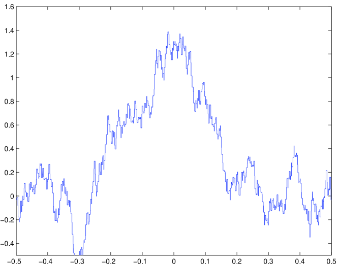
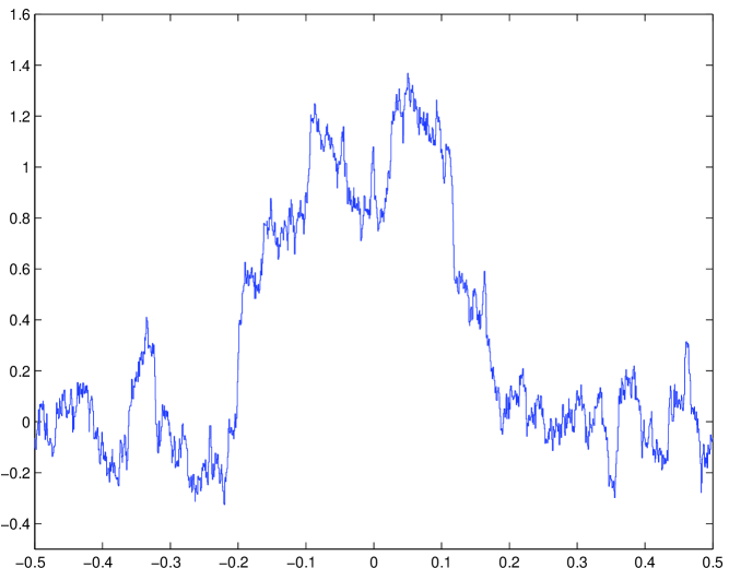
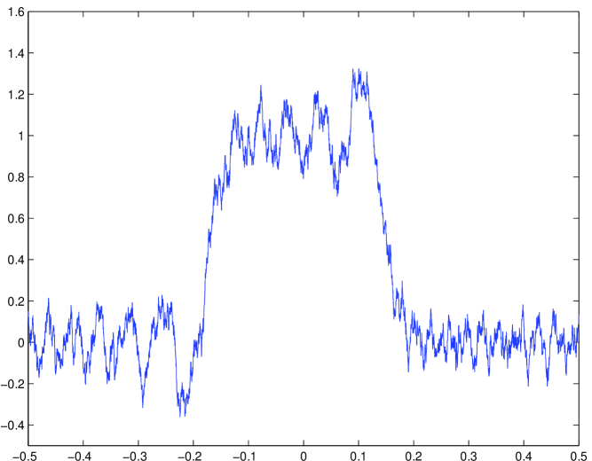
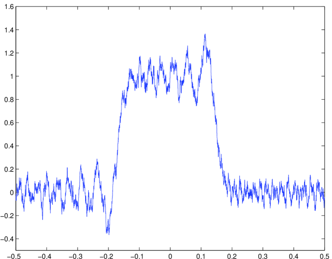
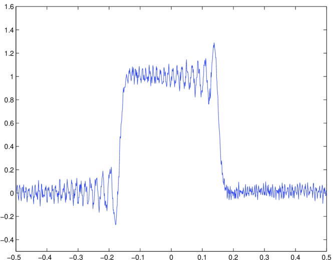
Figure 5: $n=3$ and $u/q=1/65,1/257,1/1025$ and $1/65,1/257,1/1025$

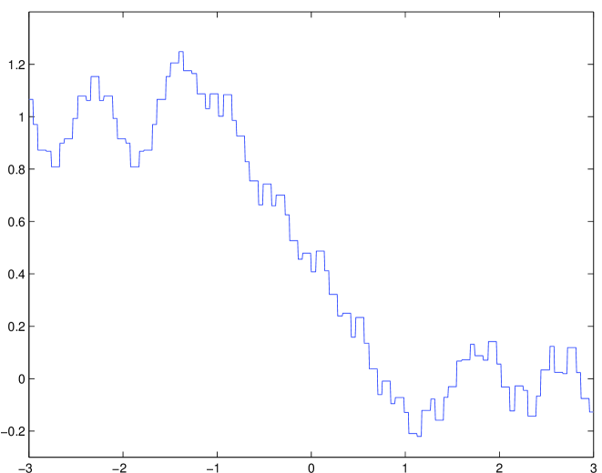
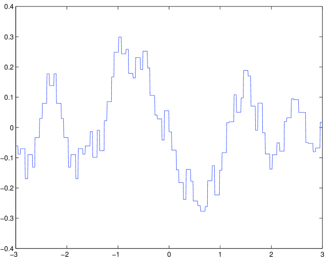
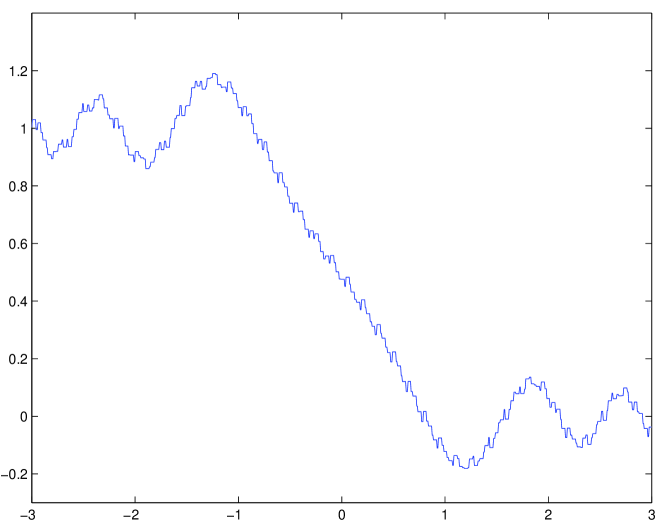
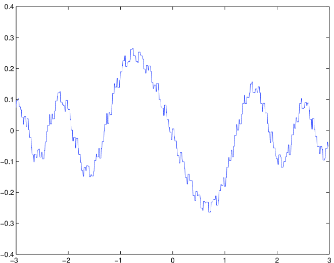
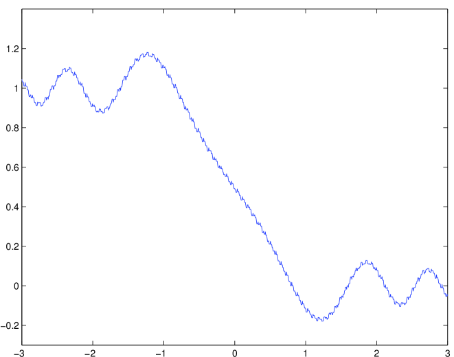
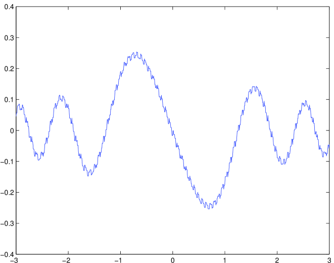
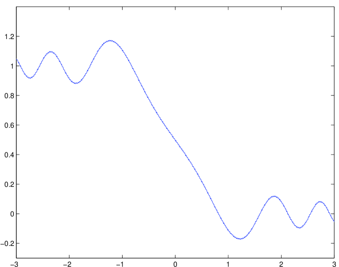
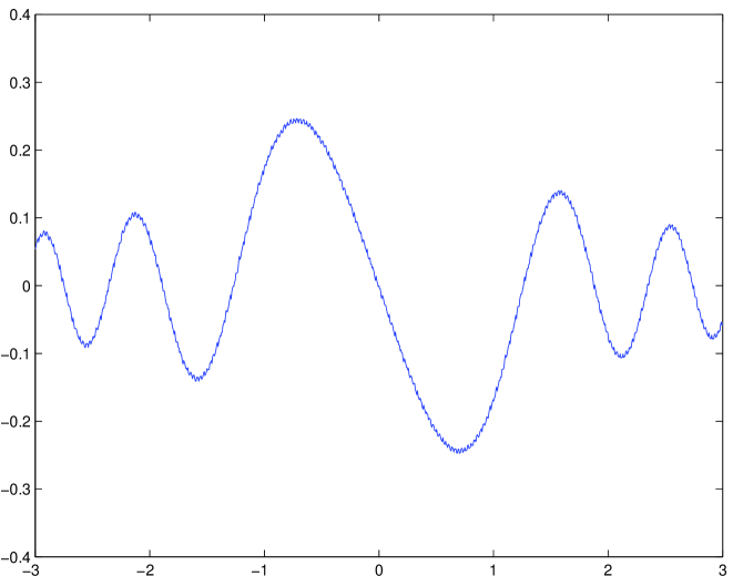
Figure 6: Real and imaginary parts of $U(t,\gamma+st^{1/2})$ for $t=1/202,1/1616,1/6464,1/51712$.

As mentioned above the proof of Theorem 1.5 uses well-known estimates for Weyl sums which are obtained in the literature using the Weyl shift method; we state the required results before proceeding. If $f(k)=\alpha_{n}k^{n}+\cdots+\alpha_{0}$, $\alpha_{n}\neq 0$, is a polynomial of degree $n\geq 2$ with real coefficients, and $k$ varies over an interval of at most $\mu$ consecutive integers, then for any $\varepsilon>0$

$$\left|\sum e(f(k))\right|^{N} \ll\mu^{N-1}+\mu^{N-n}\sum_{1\leq r_{1},\ldots,r_{n-1}\leq\mu-1}\min\left\{\mu,\frac{1}{2\{n!\alpha_{n}r_{1}r_{2}\ldots r_{n-1}\}}\right\}$$

$$\ll\mu^{N-1}+\mu^{N-n+\varepsilon}\sum_{1\leq m\leq(\mu-1)^{n-1}}\min\left\{\mu,\frac{1}{2\{n!\alpha_{n}m\}}\right\}$$ (1.17)

where $\{x\}$ denotes the distance from $x$ to the nearest integer, $N=2^{n-1}$. (Originally due to Weyl. See Titchmarsh 1986). Note also that with $\alpha_{n}=u/q$ we have

$$\sum_{1\leq m\leq(\mu-1)^{n-1}}\min\left\{\mu,\frac{1}{2\{n!\alpha_{n}m\}}\right\}= \sum_{v({\hbox{\smallrm mod}}\,q)}\min\left\{\mu,\frac{q}{2v}\right\}\sum_{\begin{subarray}{c}{\scriptstyle{1\leq m\leq(\mu-1)^{n-1}}}\\ {\scriptstyle{n!um\equiv v({\hbox{\smallrm mod}}\,q)}}\end{subarray}}1$$

$$\ll (\mu^{n-1}q^{-1}+1)(\mu+q\log q)$$ (1.18)

and hence

$$\left|\sum e(f(k))\right|^{N}\ll\mu^{N-1}+\mu^{N-n+\varepsilon}(\mu^{n-1}q^{-1}+1)(\mu+q)\log q\ .$$ (1.19)

Furthermore, if

$$\left|\alpha_{n}-\frac{h}{q}\right|\leq\frac{1}{q^{2}}\ ,\ (h,q)=1\ ,$$

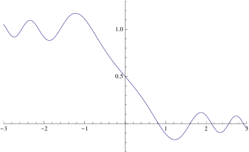
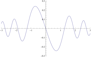
Figure 7: The real and imaginary parts of the integral for $n=2$.

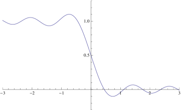
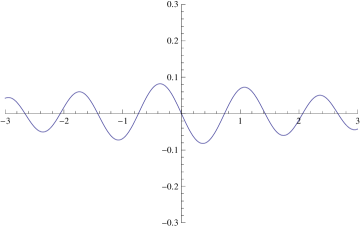
Figure 8: The real and imaginary parts of the integral for $n=6$.

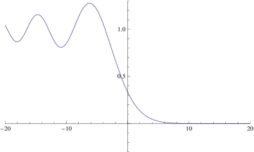
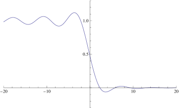
Figure 9: The integral for $n=3$ and $n=17$.

then for any $\varepsilon>0$,

$$\sum_{m=1}^{M}e(f(m))\ll\left\{M^{-1}+q^{-1}+qM^{-n}\right\}^{2^{1-n}}M^{1+\varepsilon}q^{\varepsilon}$$ (1.20)

where the implied constant depends on $\varepsilon$, and is uniform in the coefficients $\alpha_{n-1},\ldots,\alpha_{0}$. (See Hua 1965).

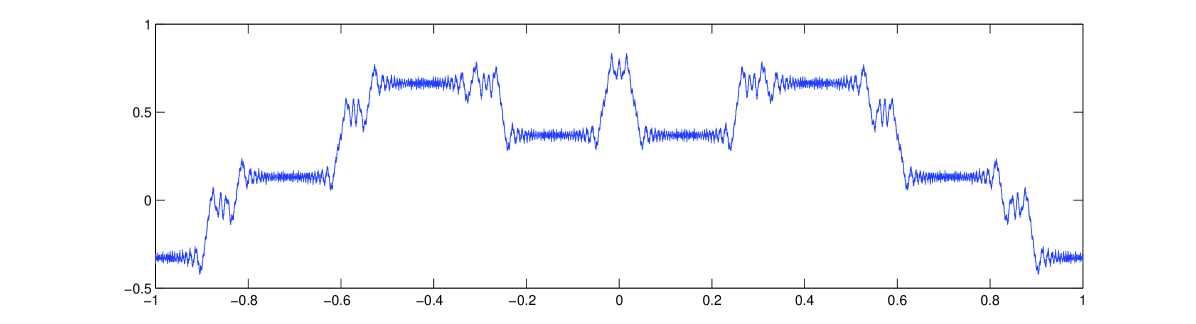
Figure 10: The graph of $U(468/3277,x)$

The structure of the paper is as follows. In section 2 we establish the properties of the sets A, ${\hbox{\script A}}_{m}$ and ${\hbox{\script B}}_{m,\alpha}$ stated in Lemma 1.2. Some of these are not strictly necessary for the remainder of the paper, but item 6 in particular is important, since it establishes that there are plenty of points in ${\hbox{\script B}}_{m,\alpha}$ through which $t$ may tend to zero. In section 3 we prove Theorem 1.4, which handles the convergence of the Fourier series at rational times, and in section 4 we use $(1.20)$ to consider convergence at irrational times in A and prove Theorem 1.3. The proof of Theorem 1.5 follows in sections 5 to 7. As is common with periodic problems, one would like to use harmonic analysis such as the Poisson summation formula to replace the series by an integral, which is more easily analysed. In this case, however, it is necessary to first separate into large and small frequencies $k$, and treat the large frequencies separately, using quite different methods for rational times and for irrational times in ${\hbox{\script B}}_{m,\alpha}$. These sections also use $(1.19)$ and $(1.20)$, although the arguments are more involved than in the proofs of convergence, and require that irrational times be in the set ${\hbox{\script B}}_{m,\alpha}$ rather than A. In section 7 we apply the Poisson summation formula to the small frequencies, and analyse the resulting integral, in essentially the same way for rational and irrational times, which completes the proof.

2. Proof of Lemma 1.2.

Items 1 and 2 are clear from the definition of the sets. To prove item 3, consider $t\notin{\hbox{\script A}}_{m}$; thus there exists $M\geq m$ for which there is no approximant $u/q$ to $t$ with $M^{\Delta}<q\leq M^{n-\Delta}$, and hence there must be consecutive convergents $u_{j}/q_{j}$ and $u_{j+1}/q_{j+1}$ for which $q_{j}\leq M^{\Delta}$ and $q_{j+1}>M^{n-\Delta}$ for some $j$. Defining

$${\hbox{\script S}}_{q,M}=\left[0,\frac{1}{qM^{n-\Delta}}\right]\cup\bigcup_{u=1}^{q-1}\left[\frac{u}{q}-\frac{1}{qM^{n-\Delta}},\frac{u}{q}+\frac{1}{qM^{n-\Delta}}\right]\cup\left[1-\frac{1}{qM^{n-\Delta}},1\right]$$

for any $q$ and $M$, by $(1.9)$ we have

$$t\in\left[0,\frac{1}{q_{j}q_{j+1}}\right]\cup\bigcup_{u=1}^{q_{j}-1}\left[\frac{u}{q_{j}}-\frac{1}{q_{j}q_{j+1}},\frac{u}{q_{j}}+\frac{1}{q_{j}q_{j+1}}\right]\cup\left[1-\frac{1}{q_{j}q_{j+1}},1\right]$$

and hence $t\in{\hbox{\script S}}_{q,M}$ for some $q,M$ with $q\leq M^{\Delta}$ and $M\geq m$. Thus

$$t\in\bigcup_{M\geq m}\bigcup_{q\leq M^{\Delta}}{\hbox{\script S}}_{q,M}$$

and since $\mu\left({\hbox{\script S}}_{q,M}\right)=M^{-n+\Delta}$, we can bound the measure of this union by

$$\mu\left(\bigcup_{M\geq m}\bigcup_{q\leq M^{\Delta}}{\hbox{\script S}}_{q,M}\right)\leq\sum_{M\geq m}M^{2\Delta-n}\ll m^{1+2\Delta-n}.$$

This proves item 3.

Suppose now that $t$ is an algebraic irrational, and recall $(1.8)$ and $(1.10)$. Since all but finitely many convergents $u_{j}/q_{j}$ differ from $t$ by at least $q_{j}^{-2-\eta}$, but by at most $q_{j}q_{j+1}^{-1}$, it follows that for all but finitely many convergents we have $q_{j+1}<q_{j}^{1+\eta}$. Now any positive number greater than 1 must fall between some $q_{j}$ and $q_{j+1}$, hence for any $M\geq 1$ there will exist $j$ for which $q_{j}<M^{n-\Delta}\leq q_{j+1}<q_{j}^{1+\eta}$ and hence $M^{(n-\Delta)/(1+\eta)}\leq q_{j}<M^{n-\Delta}$. It follows that for all sufficiently large $M$ we can find a fraction $u_{j}/q_{j}$ satisfying the conditions of Theorem 1 as long as we choose $\eta<n/\Delta-2$. This proves item 4.

Item 5 is again clear from the definitions; item 6 can be proved by adapting the argument for item 3; if $0<t<t_{0}$ and $t\notin{\hbox{\script B}}_{m,\alpha}$ there must exist $M>mt^{-\alpha}$ such that there is no approximant $u/q$ to $t$ with $M^{\Delta}<q\leq M^{n-\Delta}$. Since there is certainly an approximant with

$$\left|t-\frac{u}{q}\right|<\frac{1}{qQ}$$

where $q\leq Q$ and $Q$ is the integer part of $M^{n-\Delta}$, it must be that $q\leq M^{\Delta}$. Were $u=0$ we would have $t<(qQ)^{-1}$, which implies $t<2/(mt^{-\alpha})^{n-\Delta}$ since $Q\geq M^{n-\Delta}/2$. Thus $t<2m^{-n+\Delta}t^{\alpha(n-\Delta)}$ and hence $t^{\alpha(n-\Delta)-1}>m^{n-\Delta}/2$, which is clearly false, so $u\neq 0$. Thus $t$ is in the set

$${\hbox{\script T}}_{q,M}\subseteq\bigcup_{1\leq u\leq u_{0}}\left[\frac{u}{q}-\frac{2}{qM^{n-\Delta}},\frac{u}{q}+\frac{2}{qM^{n-\Delta}}\right]$$

for some $M\geq mt^{-\alpha}>mt_{0}^{-\alpha}$ and $q\leq M^{\Delta}$, where $u_{0}$ is such that $t_{0}<u_{0}/q+2/qM^{n-\Delta}$. The smallest element of ${\hbox{\script T}}_{q,M}$ is at least $1/2q$, so $t>1/2q$ and hence $2qt_{0}>1$. Thus we may choose $u_{0}$ to be the integer part of $2qt_{0}$ plus one, which is no more than $4qt_{0}$. The measure of ${\hbox{\script T}}_{q,M}$ is thus no more than $16t_{0}/M^{n-\Delta}$, and the measure of the union is bounded by

$$\mu\left(\bigcup_{M\geq mt_{0}^{-\alpha}}\bigcup_{q\leq M^{\Delta}}{\hbox{\script T}}_{q,M}\right)\leq\sum_{M\geq mt_{0}^{-\alpha}}\sum_{q\leq M^{\Delta}}\frac{8t_{0}}{M^{n-\Delta}}\ll t_{0}\left(mt_{0}^{-\alpha}\right)^{-n+2\Delta+1}.$$

This proves item 6, and completes the proof of Lemma 1.

3. Convergence at rational times and proof of Theorem 1.4

This follows from Theorem 2, which we prove. Fourier modes of the form $e(tP(k)+kx)$ solve the equation $LU=U_{t}$, so given $f\in{\hbox{\script D}}$, if $c_{k}$ are the Fourier coefficients of the initial condition $U(0,x)=f(x)$ then the Fourier series

$$\sum_{k}c_{k}e(tP(k)+kx)$$

is a solution to the initial value problem in the $L^{2}$ sense (as discussed in the introduction), and we wish to show it is convergent at rational times. From Katznelson 2004, for instance, we know the Fourier series for $f(x)$ is convergent, so

$$\lim_{K\rightarrow\infty}\frac{1}{q}\sum_{v({\hbox{\smallrm mod}}\,q)}G(u,v;q)\sum_{|k|\leq K}c_{k}e\left(\left(x+\frac{v}{q}\right)k\right)$$

exists and is equal to the right-hand side of $(1.15)$. On the other hand, opening $G$ and changing orders of the two sums this is equal to

$$\lim_{K\rightarrow\infty}\frac{1}{q}\sum_{|k|\leq K}c_{k}\sum_{v,w({\hbox{\smallrm mod}}\,q)}e\left(\frac{u}{q}P(w)-vw+\left(x+\frac{v}{q}\right)k\right)=\lim_{K\rightarrow\infty}\sum_{|k|\leq K}c_{k}e\left(\frac{u}{q}P(k)+xk\right)$$

which hence exists, and proves both the convergence and Theorem 1.4.

4. Convergence at irrational times and completion of the proof of Theorem 1.3

Suppose now that $P(k)$ is a monic polynomial of degree $n\geq 2$ with real coefficients. If $t\in{\hbox{\script A}}$ then there exists $m$ such that $t\in{\hbox{\script A}}_{m}$, and we consider $K>m$ and $L>K+m$, and sum by parts to obtain

$$\sum_{K<k\leq L}\frac{e(tP(k)+xk)}{k}=\frac{1}{L}\sum_{K<k\leq L}e(tP(k)+xk)+\int\limits_{K}^{L}\sum_{K<k\leq\xi}e(tP(k)+xk)\,\frac{d\xi}{\xi^{2}}.$$ (4.1)

The interval $K\leq\xi\leq K+m$ contributes at most $O(K^{-2})$ to the integral (where the implied constant depends on $m$, and hence on $t$, although this is unimportant in this section). In the remaining range $\xi>K+m$ we rewrite the sum as so that

$$S:=\sum_{K<k\leq\xi}e\left(tP(k)+xk\right)=\sum_{k\leq\xi-K}e\left(P^{*}(k)\right)$$ (4.2)

where shifting $k$ has not affected the leading coefficient of $P$, so $P^{*}(k)$ is a polynomial of the form required for $(1.19)$ and $(1.20)$, with $\alpha_{n}=t$. Choosing an approximant $u_{j}/q_{j}$ to $t$ with $(\xi-K)^{\Delta}<q_{j}\leq(\xi-K)^{n-\Delta}$ we apply $(1.20)$ and find

$$S\ll\left\{(\xi-K)^{-1}+q_{j}^{-1}+q_{j}(\xi-K)^{-n}\right\}^{2^{1-n}}(\xi-K)^{1+\varepsilon}q_{j}^{\varepsilon}\ll(\xi-K)^{1-2^{1-n}\Delta+(n+1)\varepsilon}.$$ (4.3)

Specifying $\varepsilon=\Delta/2^{n}(n+1)$ this gives $S\ll(\xi-K)^{1-\delta}$, where $\delta=\Delta/2^{n}$ and hence

$$\sum_{K<k\leq L}\frac{e(tk^{n}+xk)}{k}\ll L^{-\delta}+\int\limits_{K}^{L}\xi^{-1-\delta}d\xi\ll K^{-\delta}+L^{-\delta}\ ,$$

where we note that the constants are independent of $x$. It follows that the sequence of partial sums $(1.12)$ is a Cauchy sequence, and the series is thus convergent. The uniformity follows since none of the constants appearing depend on $x$, and hence the tail of the series for $k>K$ is uniformly bounded by $O(K^{-\delta})$.

5. Bounding the contribution from large frequencies at irrational times

Let $t\in{\hbox{\script B}}_{m,\alpha}$ as in Lemma 1.2, and suppose $(n-\Delta)^{-1}<\alpha<(n-1)^{-1}$. We define a ${\hbox{\script C}}^{\,\,\infty}$ smoothing function $\phi(x)$ such that $\phi(x)=1$ for $x\in[-1/2,1/2]$, $\phi(x)=0$ for $x\notin[-2,2]$ and $\phi(x)+\phi(x^{-1})=1$ for all $x\in{\mathbb{R}}$, so

$$U(t,x)=\frac{1}{\pi}\lim_{K\rightarrow\infty}\sum_{|k|\leq K}\!\left\{\phi\left(kt^{\alpha}\right)+\phi\left(\frac{1}{kt^{\alpha}}\right)\right\}\!\frac{\sin 2\pi\gamma k}{k}e(tk^{n}+xk)=U^{*}(t,x)+\lim_{K\rightarrow\infty}\!U_{K}(t,x)$$ (5.1)

where

$$U^{*}(t,x) =\frac{1}{\pi}\sum_{k=-\infty}^{\infty}\phi\left(kt^{\alpha}\right)\frac{\sin\gamma k}{k}e(tk^{n}+xk)\ ,$$ (5.2)

$$U_{K}(t,x) =\frac{1}{\pi}\sum_{|k|\leq K}\phi\left(\frac{1}{kt^{\alpha}}\right)\frac{\sin 2\pi\gamma k}{k}e(tk^{n}+xk).$$ (5.3)

We can write $U_{K}(t,x)$ as the difference of the two expressions

$$\frac{1}{2\pi i}\sum_{|k|\leq K}\phi\left(\frac{1}{kt^{\alpha}}\right)\frac{1}{k}e(tk^{n}+(x\pm\gamma)k)$$

and will consider only positive values of $k$; the contribution from negative values can be estimated by the same argument. By summation by parts we obtain

$$\frac{1}{2\pi i}\int\limits_{1/2t^{\alpha}}^{K}\phi\left(\frac{1}{\xi t^{\alpha}}\right)\frac{1}{\xi}d\left(\sum_{1/2t^{\alpha}<k\leq\xi}e(tk^{n}+(x\pm\gamma)k)\right)$$

$$= \frac{1}{2\pi i}\phi\left(\frac{1}{Kt^{\alpha}}\right)\frac{1}{K}\sum_{1/2t^{\alpha}<k\leq K}e(tk^{n}+(x\pm\gamma)k)$$

$$-\frac{1}{2\pi i}\int\limits_{1/2t^{\alpha}}^{K}\frac{d}{d\xi}\left\{\frac{1}{\xi}\phi\left(\frac{1}{\xi t^{\alpha}}\right)\right\}\sum_{1/2t^{\alpha}<k\leq\xi}e(tk^{n}+(x\pm\gamma)k)d\xi.$$

We can bound the remaining sums over $k$ as

$$\sum_{1/2t^{\alpha}<k\leq\xi}\!e(tk^{n}+(x\pm\gamma)k)d\xi\ll\left\{\xi^{-1}+q^{-1}+q\xi^{-n}\right\}^{1/N}\xi^{1+\varepsilon}q^{\varepsilon}$$

by $(1.20)$, where $N=2^{n-1}$. If $\xi>mt^{-\alpha}$ then we choose $q=q_{j}$ as in the definition of ${\hbox{\script B}}_{m,\alpha}$, and the sum is $O(\xi^{1-\Delta/N+\varepsilon})$; similarly for the first term with $K$ in place of $\xi$. On the other hand, if $\xi$ is smaller than this we take the value of $q$ which the lemma gives for $M=(m+1)t^{-\alpha}$, and the sum is $O\left(t^{-\alpha+\alpha\Delta/N-\varepsilon}\right)$. On taking the limit as $K\rightarrow\infty$ we now have

$$U(t,x)=U^{*}(t,x)+O(t^{\alpha\Delta/N-\varepsilon}).$$ (5.4)

6. Bounding the contribution from large frequencies at rational times

We need to provide an argument for rational times similar to that proved in the previous paragraph for irrational times; specifically we will consider $t=u/q\rightarrow 0^{+}$. The analysis is a little trickier, however, so we begin by considering the related sum given by

$$V^{*}(t,x)=\frac{1}{\pi}\sum_{k=-\infty}^{\infty}\phi\left(\frac{k}{q^{4}}\right)\frac{\sin 2\pi\gamma k}{k}e(tk^{n}+xk)$$

where $\phi$ is as used in $(5.1)$. We begin by showing

$$U(t,x)=V^{*}(t,x)+O\left(q^{-1/2}\right).$$ (6.1)

which allows us to consider the finite sum $V^{*}$ in place of $U$.

By Fourier inversion

$$V^{*}(t,x)=\frac{1}{\pi}\lim_{K\rightarrow\infty}\int\limits_{-\infty}^{\infty}{\hat{\phi}}(\eta)\sum_{|k|\leq K}\frac{\sin 2\pi\gamma k}{k}e\left(\frac{uk^{n}}{q}+\left(x+\frac{\eta}{q^{4}}\right)k\right)d\eta$$ (6.2)

where ${\hat{\phi}}$ denotes the Fourier transform $\hat{\phi}$, which can be bounded using repeated integration by parts by

$${\hat{\phi}}(\eta)=\int\limits_{-\infty}^{\infty}\phi(\xi)e(-\xi\eta)d\xi\ll\eta^{-\nu}\ ,\ \nu=0,1,2,\ldots\ .$$ (6.3)

In order to change the orders of limit and integral in $(6.2)$ we note that for any $y$

$$\frac{1}{\pi}\sum_{|k|\leq K}\frac{\sin 2\pi\gamma k}{k}e\left(tk^{n}+yk\right)=\int\limits_{0}^{1}U(t,y+u)\frac{\sin\pi(2K+1)u}{\sin\pi u}du$$ (6.4)

where $U(t,y+u)$ is piecewise constant, as discussed above, and consider the integral over $[0,1.2]$; the other half can be treated similarly. The function $g(u)=\sin(\pi u)/\pi u$ is analytic and bounded on $[0,\infty)$, and its antiderivative $G(u)$ is also bounded on $[0,\infty)$ as can be seen by observing that it tends to a finite limit as $u\rightarrow\infty$. Breaking up $(6.4)$ into the integrals over subintervals where $U(t,y+u)$ is constant, if $[a,b]$ is any such subinterval then it contributes

$$(2K+1)\int\limits_{a}^{b}U(t,y+u)\frac{\pi u}{\sin\pi u}g((2K+1)u)du.$$

Integrating by parts the integral in $(6.4)$ is $O(q)$, uniformly in $K$ and $y$. The Lebesgue Dominated Convergence Theorem can then be applied in $(6.2)$ to change the orders of limit and integral, and obtain

$$V^{*}(t,x)=\frac{1}{\pi}\int\limits_{-\infty}^{\infty}{\hat{\phi}}(\eta)\sum_{k=-\infty}^{\infty}\frac{\sin 2\pi\gamma k}{k}e\left(\frac{uk^{n}}{q}+\left(x+\frac{\eta}{q^{4}}\right)k\right)d\eta.$$ (6.5)

Applying Theorem 1.4 to the sum over $k$ it can be evaluated as a value of $U(t,x)$, and

$$V^{*}(t,x)=\frac{1}{q}\sum_{w({\hbox{\smallrm mod}}\,q)}\sum_{v({\hbox{\smallrm mod}}\,q)}e_{q}(uv^{n}-vw)\int\limits_{-\infty}^{\infty}{\hat{\phi}}(\eta)\,U\!\left(0,x+\frac{w}{q}+\frac{\eta}{q^{4}}\right)d\eta.$$ (6.6)

Using the bound $(6.3)$ the integral over $\eta$ is

$$U\!\left(0,x+\frac{w}{q}\right)\int\limits_{-\infty}^{\infty}\!\!{\hat{\phi}}(\eta)d\eta+\int\limits_{|\eta|\leq q^{2}}\!\!{\hat{\phi}}(\eta)\left\{U\!\left(0,x+\frac{w}{q}+\frac{\eta}{q^{4}}\right)-U\!\left(0,x+\frac{w}{q}\right)\right\}d\eta+O\!\left(q^{-A}\right)$$

for any $A>0$, and applying this in $(6.6)$ the first term gives $U(t,x)$ precisely, by Theorem 1.4. The integrand in the second term vanishes unless one of the conditions

$$-\gamma\leq x+w/q\leq\gamma\ ,\ -\gamma\leq x+w/q+\eta/q^{4}\leq\gamma$$

is true and the other false; this can happen in four ways, each of which implies that $w/q$ is in an interval of length $O(q^{-2})$, since the range of integration in $\eta$ is of length $q^{2}$. For sufficiently large $q$ there can be at most one $w/q$ in each of these intervals, hence these terms contribute $O\left(q^{-1/2}\right)$ to $(6.6)$. (Here we have used the bound $(1.16)$ for the complete sum over $v$ modulo $q$.) This proves $(6.1)$.

Recalling that $\phi(kt^{\alpha})+\phi(1/kt^{\alpha})=1$, for sufficiently large $q$ we have $\phi(kt^{\alpha})\phi(k/q^{4})=\phi(kt^{\alpha})$ and the definition of $V^{*}$ and $(6.1)$ imply that

$$U(t,x)=U^{*}(t,x)+\frac{1}{\pi}\sum_{k=-\infty}^{\infty}\phi\left(\frac{1}{kt^{\alpha}}\right)\phi\left(\frac{k}{q^{4}}\right)\frac{\sin 2\pi\gamma k}{k}e\left(\frac{u}{q}k^{n}+xk\right)+O(q^{-1/2})\ .$$

To estimate the second term it is sufficient to bound the sum

$$W(t,x)=\sum_{k=1}^{\infty}\phi\left(\frac{1}{kt^{\alpha}}\right)\phi\left(\frac{k}{q^{4}}\right)k^{-1}e\left(\frac{u}{q}k^{n}+yk\right)$$

where $y=x\pm\gamma$. Summing by parts in a similar fashion to section 4,

$$W(t,x) =\int\limits_{1/2t^{\alpha}}^{2q^{4}}\phi\left(\frac{1}{\xi t^{\alpha}}\right)\phi\left(\frac{\xi}{q^{4}}\right)\xi^{-1}d\left(\sum_{1/2t^{\alpha}<k\leq\xi}e\left(\frac{u}{q}k^{n}+yk\right)\right)$$

$$=-\int\limits_{1/2t^{\alpha}}^{2q^{4}}\frac{d}{d\xi}\left\{\phi\left(\frac{1}{\xi t^{\alpha}}\right)\phi\left(\frac{\xi}{q^{4}}\right)\xi^{-1}\right\}\sum_{1/2t^{\alpha}<k\leq\xi}e\left(\frac{u}{q}k^{n}+yk\right)\,d\xi$$ (6.7)

but rather than apply $(1.20)$ as we did for irrational $t$, we use $(1.19)$ and obtain

$$W(t,x)\ll \int\limits_{1/2t^{\alpha}}^{2q^{4}}\left\{\xi^{1-1/N}+\xi^{1-n/N+\varepsilon}(\xi^{n/N-1/N}q^{-1/N}+1)(\xi^{1/N}+q^{1/N})\log q\right\}\xi^{-2}d\xi$$

$$\ll \left\{t^{\alpha/N}+q^{-1/N}+t^{\alpha n/N}q^{1/N}\right\}q^{\varepsilon}.$$

Since $\alpha<1/(n-1)\leq 1$, we have $t^{\alpha}>t>q^{-1}$ so the second term can be dropped, as can the error term from $(6.1)$. Furthermore the second term dominates the third only if $t<q^{-1/\alpha(n-1)}<q^{-1}$, which is false for sufficiently large $q$, so $t^{\alpha}>t^{1/(n-1)}>q^{-1/(n-1)}$, and

$$U(t,x)=U^{*}(t,x)+O\left(t^{\alpha n/N}q^{1/N+\varepsilon}\right).$$ (6.8)

Supposing now that $t\leq mq^{-1/\alpha(n-\Delta)}$ this error term is $O(t^{\alpha\Delta/N-\varepsilon})$ as in $(5.4)$ and Theorem 1.5.

7. An asymptotic estimate for $U^{*}(t,x)$

To estimate $U^{*}$ we write it as

$$U^{*}(t,x)=\int\limits_{x-\gamma}^{x+\gamma}\sum_{k=-\infty}^{\infty}\phi\left(kt^{\alpha}\right)e(tk^{n}+\eta k)d\eta$$

and consider the inner sum. Note that for this part of the analysis it makes no difference whether $t$ is rational or irrational. Applying the Poisson summation formula

$$\sum_{k}\phi\left(kt^{\alpha}\right)e(tk^{n}+\eta k)=\sum_{m}\int\limits_{-\infty}^{\infty}\phi\left(yt^{\alpha}\right)e(ty^{n}+(\eta-m)y)dy=t^{-\alpha}\sum_{m}\int\limits_{-\infty}^{\infty}\phi(y)e(F_{m}(y))dy$$

where $F_{m}(y)=t^{1-n\alpha}y^{n}+(\eta-m)t^{-\alpha}y$. For $m\neq 0$

$$\left|\eta-m\right|\geq|m|-(|x|+\gamma)\geq 1-(|x|+\gamma)>0$$

so for sufficiently small $t$

$$\left|F_{m}^{\prime}(y)\right|\geq|m-\eta|t^{-\alpha}-nt^{1-n\alpha}|y|^{n-1}\geq\frac{1}{2}|m-\eta|t^{-\alpha}\geq\frac{1}{2}\left(|m|-(|x|+\gamma)\right)t^{-\alpha}$$

since $\alpha<1/(n-1)$. Thus for $m\neq 0$, $F_{m}^{\prime}(y)$ does not vanish in the region of integration and we can integrate by parts twice and find

$$\int\limits_{-\infty}^{\infty}\!\phi(y)e(F_{m}(y))dy=-\frac{1}{4\pi^{2}}\!\int\limits_{-\infty}^{\infty}\!\frac{d}{dy}\!\left\{\frac{1}{F_{m}^{\prime}(y)}\frac{d}{dy}\!\left\{\frac{\phi(y)}{F_{m}^{\prime}(y)}\right\}\right\}e(F_{m}(y))dy\ll\frac{t^{2\alpha}}{(|m|-(|x|+\gamma))^{2}}$$

so the contribution from all $m\neq 0$ is thus

$$t^{-\alpha}\int\limits_{x-\gamma}^{x+\gamma}\sum_{m\neq 0}\int\limits_{-\infty}^{\infty}\phi(y)e(F_{m}(y))dy\ll t^{\alpha}\sum_{m=1}^{\infty}\left(|m|-(|x|+\gamma)\right)^{-2}\ll t^{\alpha},$$ (7.1)

where the implied constant depends on $\gamma$ but not on $x$, and hence

$$U^{*}(t,x) =t^{-\alpha}\int\limits_{x-\gamma}^{x+\gamma}\int\limits_{-\infty}^{\infty}\phi(y)e(t^{1-n\alpha}y^{n}+\eta t^{-\alpha}y)dy\,d\eta+O\left(t^{\alpha}\right)$$

$$=\int\limits_{(x-\gamma)t^{-1/n}}^{(x+\gamma)t^{-1/n}}\int\limits_{-\infty}^{\infty}\phi(yt^{\alpha-1/n})e(y^{n}+\eta y)dy\,d\eta+O\left(t^{\alpha}\right).$$ (7.2)

If $n$ is even, the equation $ny^{n-1}+\eta=0$ has a unique solution $y_{0}=(-\eta/n)^{1/(n-1)}$; if $n$ is odd there at most two solutions, given by $\pm y_{0}$ if present. In either case the solutions are in the range of support of $\phi(yt^{\alpha-1/n})$ if and only if $|\eta|\leq n2^{n-1}t^{1-1/n-\alpha(n-1)}$. If $x>\gamma$ then for sufficiently small $t$ we have $(x-\gamma)t^{-1/n}>n2^{n}t^{1-1/n-\alpha(n-1)}$, since $\alpha<1/(n-1)$, so there are no solutions $y_{0}$ in the support of $\phi(yt^{\alpha-1/n})$, and

$$|ny^{n-1}+\eta|\geq\eta-ny^{n-1}>\eta-n2^{n-1}t^{1-1/n-\alpha(n-1)}>\eta-\frac{x-\gamma}{2}t^{-1/n}>\eta/2.$$

Integrating by parts twice in $y$ we can now bound the integral in $(7.2)$ by

$$-\frac{1}{4\pi^{2}}\int\limits_{(x-\gamma)t^{-1/n}}^{(x+\gamma)t^{-1/n}}\int\limits_{-\infty}^{\infty}\frac{d}{dy}\left\{\frac{1}{ny^{n-1}+\eta}\frac{d}{dy}\left\{\frac{\phi(yt^{\alpha-1/n})}{ny^{n-1}+\eta}\right\}\right\}e(y^{n}+\eta y)dy\,d\eta\ll t^{\alpha}(x-\gamma)^{-1}\ .$$

A similar calculation shows that if $x<-\gamma$ then the integral is $O(t^{\alpha}|\gamma+x|^{-1})$; we can combine these two cases with $(7.1)$ to give $U^{*}(t,x)\ll t^{\alpha}|x^{2}-\gamma^{2}|^{-1}$ where the implied constant depends on $\gamma$.

On the other hand, if $-\gamma<x<\gamma$ then this same reasoning applies to the two tails $\eta>(x+\gamma)t^{-1/n}$ and $\eta<(x-\gamma)t^{-1/n}$ so that in this case

$$U^{*}(t,x)=\int\limits_{-\infty}^{\infty}\int\limits_{-\infty}^{\infty}\phi(yt^{\alpha-1/n})e(y^{n}+\eta y)dy\,d\eta+O\left(t^{\alpha}|x^{2}-\gamma^{2}|^{-1}\right)\ .$$

The inner integral in the remaining expression is the Fourier transform of $\phi(yt^{\alpha-1/n})e(y^{n})$, hence the outer integral is inverting the transform and gives the value of the original function at $0$, so combining these estimates with $(7.1)$ we have

$$U^{*}(t,x)=\begin{cases}1+O\left(t^{\alpha}|x^{2}-\gamma^{2}|^{-1}\right)&\text{if $|x|<\gamma$}\\ O\left(t^{\alpha}|x^{2}-\gamma^{2}|^{-1}\right)&\text{if $|x|>\gamma$}\end{cases}$$

and combining this last with $(5.4)$ and $(6.8)$ we obtain the first claim in Theorem 1.5.

The transition between these two cases is the main concern in Theorem 1.5. We will consider $x$ near $\gamma$, omitting the details for $x$ near $-\gamma$, which are very similar. If we renormalise values of $x$ as $x=\gamma+st^{1/n}$ for $s$ in some fixed interval $[-S,S]$, then $(7.2)$ becomes

$$U^{*}\left(t,\gamma+st^{1/n}\right)=\int\limits_{s}^{s+2\gamma t^{-1/n}}\int\limits_{-\infty}^{\infty}\phi(yt^{\alpha-1/n})e(y^{n}+\eta y)dy\,d\eta+O\left(t^{\alpha}\right).$$

Since $1/n<\alpha<1/(n-1)$ by hypothesis, $-1<(1-\alpha n)(n-1)<0$, and hence for $\eta>s+2\gamma t^{-1/n}$

$$\left|ny^{n-1}+\eta\right|\gg t^{-1/n}-t^{(1-\alpha n)(n-1)/n}\gg t^{-1/n}.$$

Integrating by parts twice as above,

$$\int\limits_{s+2\gamma t^{-1/n}}^{\infty}\int\limits_{-\infty}^{\infty}\phi(yt^{\alpha-1/n})e(y^{n}+\eta y)dy\,d\eta\ll t^{\alpha}$$

and hence

$$U^{*}\left(t,\gamma+st^{1/n}\right)=\int\limits_{s}^{\infty}\int\limits_{-\infty}^{\infty}\phi(yt^{\alpha-1/n})e(y^{n}+\eta y)dy\,d\eta+O\left(t^{\alpha}\right)\ .$$

Suppose $n$ is even. Were the integral in $\eta$ over $(-\infty,\infty)$ then the double integral would be the Fourier inverse at zero of the Fourier transform of $\phi(yt^{\alpha-1/n})e(y^{n})$, so the double integral would be equal to $1$. Since the integral over $\eta\in(0,\infty)$ is half this,

$$U^{*}\left(t,\gamma+st^{1/n}\right) =\frac{1}{2}-\int\limits_{0}^{s}\int\limits_{-\infty}^{\infty}\phi(yt^{\alpha-1/n})e(y^{n}+\eta y)dy\,d\eta+O\left(t^{\alpha}\right)$$

$$=\frac{1}{2}-\frac{1}{2\pi}\int\limits_{-\infty}^{\infty}\phi(yt^{\alpha-1/n})e(y^{n})\sin 2\pi sy\,\frac{dy}{y}+O\left(t^{\alpha}\right).$$

The calculation is completed by noting that by integration by parts

$$\int\limits_{0}^{\infty}\phi(1/yt^{\alpha-1/n})e(y^{n}+sy)\,\frac{dy}{y}=-\int\limits_{0}^{\infty}\frac{d}{dy}\left\{\frac{\phi(1/yt^{\alpha-1/n})}{y\left(ny^{n-1}+s\right)}\right\}e(y^{n}+sy)\,dy\ll t^{\alpha n-1}$$

and similarly for $y^{n}-sy$, and hence

$$U^{*}\left(t,\gamma+st^{1/n}\right)=\frac{1}{2}-\frac{1}{\pi}\int\limits_{0}^{\infty}e(y^{n})\sin 2\pi sy\,\frac{dy}{y}+O\left(t^{\alpha n-1}\right).$$

On the other hand, if $n$ is odd then $(7.2)$ becomes

$$U^{*}\left(t,\gamma+st^{1/n}\right) =\int\limits_{s}^{\infty}\int\limits_{-\infty}^{\infty}\phi(yt^{\alpha-1/n})\cos 2\pi(y^{n}+\eta y)dy\,d\eta+O\left(t^{\alpha}\right)$$

$$=\frac{1}{2}-\int\limits_{0}^{s}\int\limits_{-\infty}^{\infty}\phi(yt^{\alpha-1/n})\cos 2\pi(y^{n}+\eta y)dy\,d\eta+O\left(t^{\alpha}\right)$$

$$=\frac{1}{2}-\frac{1}{2\pi}\int\limits_{-\infty}^{\infty}\phi(yt^{\alpha-1/n})\sin 2\pi(y^{n}+\eta y)\frac{dy}{y}+O\left(t^{\alpha}\right)$$

which gives the form in Theorem 1.5.

References

Abramovitz, M & Stegun, I. 1972, Handbook of Mathematical Functions, US Govt. Printing Office.

Arkhipov, G. I. & Oskolkov, K. I. 1989, On a special trigonometric series and its applications, Math. USSR Sbornik, 62 (1), 145-155

Berry, M. V. & Klein, S. 1996, Integer, fractional and fractal Talbot effects, Journal of Modern Optics 43, no. 10, 2139–2164.

DiFranco, J. C. & McLaughlin, K. T.-R., 2005, A nonlinear Gibbs-type phenomenon for the defocusing nonlinear Schrödinger equation, Int. Math. Res. Pap. 8, 403-459

Hardy, G. H. & E. M. Wright, E. M. 1979, An introduction to the theory of numbers, 5th edition, OUP.

Hua, L.-K. 1965, Additive theory of prime numbers, AMS.

Hua, L.-K. 1982, Introduction to number theory, Springer.

Kapitanski, L & Rodnianski, I 1999, Does a quantum particle know the time?, Proceedings of the workshop on Emerging Applications of Number Theory, IMA Volumes in Mathematics and its Applications 109, 355-371.

Katznelson, Y 2004, An introduction to harmonic analysis, 3rd edition, CUP

Olver, P 2010, Dispersive quantization, Amer. Math. Monthly 117, 599-610

Oskolkov, K. I. 1992, A class of I. M. Vinogradov’s series and its applications in harmonic analysis, Springer Series in Computational Mathematics, 19, Progress in Approxi mation Theory, an International perspective (A. A. Gonchar and E. B. Sta, eds.), Springer-Verlag, New York.

Rodnianski, I. 2000, Fractal solutions of the Schrödinger equation, in: Nonlinear PDE’s, dynamics and continuum physics (South Hadley, MA, 1998), 181Ð187, Contemp. Math. 255, Amer. Math. Soc., Providence, RI, 2000.

Rodnianski, I. 1999, Continued fractions and Schrödinger evolution, Proceedings of the conference on Continued Fractions: from Analytic Number Theory to Constructive Approximations (eds. B. Berndt, F. Gesztesy), Contemp. Math. 236 (1999), 311-323.

Roth, K. F. 1955, Rational approximations to algebraic numbers, Mathematika 2 1-20; corrigendum, 168

Schmidt, W. 2004, Equations over finite fields, 2nd edition, Kendrick Press

Stein, E.M. and Wainger, S. 1990, Discrete analogues of singular Radon transforms, Bull. Amer. Math. Soc. 23 , 537-544.

Talbot, H. F. 1836, Facts relating to Optical Science. No. IV, Phil. Mag. 9, 401-407.

Titchmarsh, E. C. 1986, The theory of the Riemann zeta-function, 2nd edition, OUP.