Analysis and Improvement of Low Rank Representation for Subspace segmentation

Abstract

We analyze and improve low rank representation (LRR), the state-of-the-art algorithm for subspace segmentation of data. We prove that for the noiseless case, the optimization model of LRR has a unique solution, which is the shape interaction matrix (SIM) of the data matrix. So in essence LRR is equivalent to factorization methods. We also prove that the minimum value of the optimization model of LRR is equal to the rank of the data matrix. For the noisy case, we show that LRR can be approximated as a factorization method that combines noise removal by column sparse robust PCA. We further propose an improved version of LRR, called Robust Shape Interaction (RSI), which uses the corrected data as the dictionary instead of the noisy data. RSI is more robust than LRR when the corruption in data is heavy. Experiments on both synthetic and real data testify to the improved robustness of RSI.

1 Introduction

In many computer vision and machine learning problems, one often assumes that the data is drawn from a union of multiple linear subspaces. Thus subspace segmentation of such data has been studied extensively. The existing methods for subspace segmentation can be roughly divided into four groups: statistical learning based methods ([1, 2]), factorization based methods ([3, 4, 5]), algebra based methods [6], and sparsity based methods (e.g., SSC [7] and LRR [8]).

LRR [8] is a recently proposed method and is reported to have excellent performance on both synthetic and benchmark data sets. For the noiseless case, LRR takes the data itself as a dictionary and seeks the representation matrix with the lowest rank. LRR can also handle noisy data by adding a (2,1)-norm term to the objective function in order to make the noise column sparse. The experimental results show that it is both robust and accurate.

However, the motivation to utilize low rank criterion in LRR remains vague. In [8], the authors only proved that for noiseless case, the convex optimization model of LRR admits a block diagonal solution, which is the representation they seek. As the nuclear norm is not strongly convex, it is unclear whether such a solution is unique and what it actually is. If the uniqueness is not guaranteed, we may be at risk of finding a non-block-diagonal solution. In this case the clustering information will not be revealed. In the case of noisy data, the authors simply added a (2,1)-norm term to the objective function without providing sufficient insight to why such treatment can work well.

Our Contributions

In this paper, we present detailed analysis of LRR. We find that although LRR was categorized by the authors of [8] as a sparsity based method, it is actually closely related to the factorization methods. Our main contributions are:

1. We prove that in the noiseless case, LRR has a unique solution, which is exactly the shape interaction matrix of the data matrix. Consequently, the minimum objective function value is the rank of the data matrix.

2. For the noisy case, we show that LRR can be roughly regarded as first applying a column sparse robust PCA [9] to remove noise, and then performing segmentation on the corrected data.

3. We propose a modified model, called Robust Shape Interaction (RSI) due to its dependence on the shape interaction matrix, as an improvement of LRR. Our experiments show that RSI is more robust and has better performance than LRR.

The remainder of this paper is organized as follows. Section 2 reviews the related state-of-the-art methods. Section 3 studies the relationship between LRR and factorization methods. Then Section 4 introduces RSI as an improvement of LRR. The simulation results on synthetic and real data are shown in Section 5. Finally, Section 6 concludes the paper.

2 Review of LRR and Factorization Methods

2.1 Basic Subspace Segmentation Problem

Let $X=[x_{1},x_{2},...,x_{n}]$ be a collection of $m$ dimensional data vectors drawn from a union of linear subspaces $\{\mathcal{S}_{i}\}_{i=1}^{k}$, where the dimension of $\mathcal{S}_{i}$ is $r_{i}$. The task of subspace segmentation (or clustering) is to cluster the vectors in $X$ according to those subspaces.

For notational simplicity, we may assume $X=[X_{1},X_{2},...,X_{k}]$, where $X_{i}$ consists of the vectors in $\mathcal{S}_{i}$. For LRR and factorization methods, it is assumed that the subspaces are independent.

Denote $d_{i}$ as the number of vectors in $X_{i}$. Then there must be at least one block diagonal matrix $Z=\operatorname{diag}\{Z_{1},Z_{2},...,Z_{k}\}$ satisfying

$$X=XZ,$$ (1)

where the size of the $i$-th block $Z_{i}$ is $d_{i}\times d_{i}$. Equation (1) actually has an infinite amount of solutions. Any solution is called a representation matrix. Note that the block diagonal structure of $Z$ directly induces segmentation of the data (each block corresponds to a cluster). So the clustering task is equivalent to finding a block diagonal representation matrix $Z$.

2.2 Subspace Segmentation by Low-rank Representation

As the solution to (1) is not unique, LRR [8] seeks the lowest rank representation matrix. When the data is noiseless, LRR solves the following optimization problem:

$$\min_{Z}\|Z\|_{*},\ \ \ \ s.t.\ \ X=XZ,$$ (2)

where $\|\cdot\|_{*}$ denotes the nuclear norm. It was proved in [8] that the solution set of (2) includes at least a block diagonal representation matrix $Z^{0}$ that can be used for clustering.

When the data is noisy, the optimization model of LRR is formulated as:

$$\min_{Z,E}\|Z\|_{*}+\lambda\|E\|_{2,1},\ \ \ \ s.t.\ \ X=XZ+E,$$ (3)

where $\|E\|_{2,1}=\sum_{j=1}^{n}\sqrt{\sum_{i=1}^{n}(E_{ij}^{2})}$ is the (2,1)-norm. Minimizing the (2,1)-norm of noise is to meet the assumption that the corruptions are “sample specific” [8], i.e., some data vectors are corrupted and the others are clean. Since in this case, the solution $Z^{*}$ to (3) may not be block diagonal, it is recognized as an affinity matrix instead and spectral clustering methods are applied to $|Z^{*}|+|(Z^{*})^{\prime}|$ to obtain a block diagonal matrix, where ^′ denotes the matrix or vector transpose and $|A|$ denotes a matrix whose entries are the absolute values of $A$.

2.3 Factorization Methods and Shape Interaction Matrix

Factorization based methods build a similarity matrix by factorizing the data matrix and then applying spectral clustering to the similarity matrix for clustering. This similarity matrix, which is called the shape interaction matrix (SIM) [3] in computer vision, is defined as $SIM(X)=V_{r}V_{r}^{\prime}$, where $X=U_{r}S_{r}V_{r}^{\prime}$ is the skinny singular value decomposition (SVD) of $X$ and $r$ is the rank of $X$. When the data is noiseless, we have [3]:

Theorem 2.1

(Costeira and Kanade) Under the assumption that the subspaces are independent and the data $X$ is clean, $SIM(X)$ is a block diagonal matrix that has exactly $k$ blocks. Moreover, the $i$-th block on its diagonal is of size $d_{i}\times d_{i}$.

We can further have:

Theorem 2.2

The rank of the $i$-th diagonal block of $SIM(X)$ is $r_{i}$.

Proof: We partition $V_{r}^{\prime}$ as $V_{r}^{\prime}=[V_{r,1}^{\prime},V_{r,2}^{\prime},...,V_{r,k}^{\prime}]$, where the number of columns in $V_{r,i}^{\prime}$ is $d_{i}$. Then $V_{r,i}V_{r,i}^{\prime}$ is the $i$-th diagonal block of $SIM(X)$ and $X_{i}=U_{r}S_{r}V_{r,i}^{\prime}$. We can also have $V_{r,i}^{\prime}=S_{r}^{-1}U_{r}^{\prime}X_{i}$. So $\operatorname{rank}(V_{r,i}^{\prime})=\operatorname{rank}(X_{i})=r_{i}$. The theorem is proved by using the relationship $\operatorname{rank}(V_{r,i}V_{r,i}^{\prime})=\operatorname{rank}(V_{r,i}^{\prime})$.

$\Box$

Theorem 2.1 is the theoretical foundation of why SIM can serve as the similarity matrix for subspace segmentation. When the data contains noise, the SIM of the data matrix can still be computed. Although in this case the SIM may not be block diagonal, it can be made block diagonal, e.g., by applying spectral clustering methods.

3 Relationship between LRR and Factorization Methods

Though LRR was proposed as a sparsity based method, we show in this section that it is equivalent to the factorization methods. This is revealed by the following theorem:

Theorem 3.1

The shape interaction matrix $SIM(X)$ is the unique solution to the optimization problem (2) and the minimum objective function value is $\operatorname{rank}(X)$.

Proof: Let $[U_{x},S_{x},V_{x}]$ and $[U_{z},S_{z},V_{z}]$ be the full SVD of $X$ and $Z$, respectively. Denote $M=V_{x}^{\prime}V_{z}$ and $N=V_{x}^{\prime}U_{z}$. They are both orthogonal matrices. Then $X=XZ$ is equivalent to

$$S_{x}M=S_{x}NS_{z}.$$ (4)

Suppose $X$ is of rank $r$ and $M$ and $N$ are partitioned as $M=\left(\begin{array}[]{c}M_{r}\\ M_{n-r}\end{array}\right)$ and $N=\left(\begin{array}[]{c}N_{r}\\ N_{n-r}\end{array}\right)$, respectively, where $M_{r}$ means that it consists of $r$ rows of $M$, etc. Then (4) reduces to

$$M_{r}=N_{r}S_{z}.$$ (5)

Now consider (2). Since

$$NS_{z}M^{\prime}=\left(\begin{array}[]{cc}N_{r}S_{z}M_{r}^{\prime}&N_{r}S_{z}M_{n-r}^{\prime}\\ N_{n-r}S_{z}M_{r}^{\prime}&N_{n-r}S_{z}M_{n-r}^{\prime}\\ \end{array}\right),$$ (6)

by Lemma 3.1 in [8], we have

$$\|N_{r}S_{z}M_{r}^{\prime}\|_{*}\leq\|NS_{z}M^{\prime}\|_{*}-\|N_{n-r}S_{z}M_{n-r}^{\prime}\|_{*}.$$

As $\|N_{r}S_{z}M_{r}^{\prime}\|_{*}=\|M_{r}M_{r}^{\prime}\|_{*}=r$, where (5) is applied, and $\|NS_{z}M^{\prime}\|_{*}=\|S_{z}\|_{*}=\|Z\|_{*}$, the above inequality reduces to

$$r\leq\|Z\|_{*}-\|N_{n-r}S_{z}M_{n-r}^{\prime}\|_{*}\leq\|Z\|_{*}.$$ (7)

Noticing $\|SIM(X)\|_{*}=r$ and $X=X\cdot SIM(X)$, we conclude that the optimal $Z$ must satisfy $\|Z\|_{*}=r$, i.e., the minimum objective function value is $\operatorname{rank}(X)$, and $SIM(X)$ is one of the optimal solutions.

Next, we prove that $SIM(X)$ is the unique solution to (2). Suppose that $Z_{0}$ is a solution to (2). First, by (5) $N_{r}S_{z_{0}}M_{n-r}^{\prime}=M_{r}M_{n-r}^{\prime}=0$. Note that here and in the sequel, $N_{r}$ and $M_{n-r}$ depend on $z_{0}$. Second, since $\|Z_{0}\|_{*}=r$, from (7) we have $N_{n-r}S_{z_{0}}M_{n-r}^{\prime}=0$. Thus (6) reduces to

$$NS_{z_{0}}M^{\prime}=\left(\begin{array}[]{cc}N_{r}S_{z_{0}}M_{r}^{\prime}&0\\ N_{n-r}S_{z_{0}}M_{r}^{\prime}&0\\ \end{array}\right),$$ (8)

which implies the rank of $Z_{0}$ must be $r$, i.e., $S_{z_{0}}$ has only $r$ nonzero entries on its diagonal. We then further partition $M_{r}$ and $N_{r}$ as $M_{r}=[M_{r,r},M_{r,n-r}]$ and $N_{r}=[N_{r,r},N_{r,n-r}]$, respectively, where $M_{r,r}$ consists of $r$ columns of $M_{r}$, etc., and write $S_{z_{0}}=\operatorname{diag}\{z_{1},z_{2},...,z_{r},0,...,0\}$, where $z_{1}\geq z_{2}\geq...\geq z_{r}>0$. Then by comparing both sides of (5) we have $M_{r,n-r}=0$. So $M_{r,r}$ is an orthogonal matrix and $M_{r,r}=N_{r,r}\operatorname{diag}\{z_{1},z_{2},...,z_{r}\}$. We further denote $M_{r,r}^{r}$ and $N_{r,r}^{r}$ as the last columns of $M_{r,r}$ and $N_{r,r}$, respectively. Then $M_{r,r}^{r}=z_{r}N_{r,r}^{r}$ and thus we have

$$z_{r}=\frac{\|M_{r,r}^{r}\|_{2}}{\|N_{r,r}^{r}\|_{2}}=\frac{1}{\|N_{r,r}^{r}\|_{2}}\geq 1,$$ (9)

where $\|\cdot\|_{2}$ denotes the 2-norm of a vector. The last inequality holds because $N_{r,r}^{r}$ is part of a column of the orthogonal matrix $N$. Since $z_{r}$ is the smallest nonzero singular value of $Z_{0}$ and $\|Z_{0}\|_{*}=r$, (9) implies that all the nonzero singular values of $Z_{0}$ must be 1. So we conclude that $M_{r,r}=N_{r,r}$, $S_{z_{0}}=\operatorname{diag}\{I_{r},0_{n-r}\}$ and hence both $M$ and $N$ are block diagonal. Finally,

$$\begin{array}[]{l}Z_{0}=V_{z_{0}}S_{z_{0}}U_{z_{0}}^{\prime}=(V_{x}N)S_{z_{0}}(V_{x}M)^{\prime}=V_{x}(NS_{z_{0}}M^{\prime})V_{x}^{\prime}\\ =V_{x}\operatorname{diag}\{I_{r},0_{n-r}\}V_{x}^{\prime}=V_{r}V_{r}^{\prime}=SIM(X).\end{array}$$

$\Box$

As the uniqueness of the solution to LRR is guaranteed, we can always use LRR to cluster clean data. Moreover, that the solution is $SIM(X)$ can help us to understand the noisy LRR model (3).

Understanding the Noisy LRR Model

Now consider the noisy case. It was not completely clear why solving (3) is effective in removing the column sparse noise. Note that LRR uses the noisy data $X$ itself as the dictionary instead of the clean data $D$, which is not quite reasonable when the noise is heavy or the percentage of outliers is relatively large. If we use the clean data as the dictionary, the noisy LRR model (3) would change to:

$$\min_{Z,D,E}\|Z\|_{*}+\lambda\|E\|_{2,1},\ \ \ \ s.t.\ \ D=DZ,\ \ X=D+E.$$ (11)

By Theorem 3.1 it is straightforward to see that (11) is equivalent to

$$\min_{D,E}\,\operatorname{rank}(D)+\lambda\|E\|_{2,1},\ \ \ s.t.\ \ X=D+E,$$ (12)

and $Z=SIM(D)$. Model (12) is very similar to the robust PCA model [9]. It would decompose the data into two parts: one is of low rank and the other is column sparse. So we call problem (12) column sparse robust PCA (CSRPCA). Denote $\mathcal{S}=\oplus_{i=1}^{k}\mathcal{S}_{i}$. Then the noise in the data can be decomposed into parts: $E=E_{s}+E^{\perp}_{s}$, where each column of $E_{s}$ belongs to space $\mathcal{S}$ and each column of $E^{\perp}_{s}$ is orthogonal to $\mathcal{S}$. As rank minimization methods are to remove noise outside the span of the clean data, CSRPCA is effective in removing $E^{\perp}_{s}$ but is unable to remove $E_{s}$. However in many real problems, the dimension of $\mathcal{S}$ (i.e., the rank $r$ of clean data) is much smaller than the dimension of data. So with high probability, $\|E_{s}\|_{F}$ is much smaller than $\|E^{\perp}_{s}\|_{F}$, where $\|\cdot\|_{F}$ denotes the Frobenius norm. Consequently, CSRPCA is able to remove most of the noise.

So we can see that the LRR model for noisy data is an approximation of (11). Solving (11) is equivalent to first applying CSRPCA to remove the noise that is orthogonal to the space spanned by the clean data, then computing the SIM to build the affinity matrix. Since the noise level is greatly reduced, spectral clustering methods on such an affinity matrix can be very effective to segment the data into subspaces. This explains why LRR can have good performance on noisy data.

4 RSI: an Improved Version of LRR

That $X$ itself can be used as the dictionary is based on the assumption that the percentage of outliers is small and the noise level is low. When this is not true, a more reasonable formulation is (11), or equivalently (12). Following the convention, we may replace the rank function in (12) with the nuclear norm, giving rise to the following convex optimization problem:

$$\min_{D,E}\|D\|_{*}+\lambda\|E\|_{2,1},\ \ \ s.t.\ \ X=D+E.$$ (13)

Similar to robust PCA [9], the above problem can be solved by the inexact augmented Lagrange Multiplier algorithm [10], which is based on the following Lagrangian function:

$$\begin{array}[]{rcl}L(D,E,Y)&\!\!=&\!\!\|D\|_{*}+\lambda\|E\|_{2,1}+\left\langle{Y,X-D-E}\right\rangle\\ &&+\frac{\mu}{2}\|X-D-E\|_{F}^{2},\end{array}$$

where $Y$ is the Lagrange multiplier, $\mu$ is a positive penalty parameter, and $\langle A,B\rangle=\operatorname{tr}(A^{\prime}B)$ is the inner product of matrices.

When the “clean” data $D$ is obtained, its representation matrix can be obtained as $Z=SIM(D)$. As $D$ still contains noise $E_{s}$, $Z$ may not be a block diagonal matrix. Like LRR and SSC [7], spectral clustering is also applied to $|Z|$ to reveal the subspace clustering information. Note that as $SIM(D)$ is symmetric, we do not have to use $|Z|+|Z^{\prime}|$ as the affinity matrix. We call this method Robust Shape Interaction (RSI). The pseudo-code for RSI is presented in Algorithm 1, where $\Theta_{\varepsilon}(x)=\max(|x|-\varepsilon,0)\operatorname{sgn}(x)$ is the thresholding operator. Readers are encouraged to refer to [10] and [8] for the deduction of the formulae in Algorithm 1.

Although SRI does not make a big change to LRR, as CSRPCA removes most of the noise and SRI uses relatively clean data as the dictionary, RSI is more robust than LRR, particularly when the data is heavily corrupted.

Algorithm 1 Robust Shape Interaction

  Input: data matrix $X$, parameter $\lambda>0$.

  Initialize : $E_{0}$, $Y_{0}$, $\mu_{0}>0$, $\mu_{\max}>\mu_{0}$, $\rho>1$, $\epsilon>0$.

  while $\|X-D_{k}-E_{k}\|_{\infty}\geq\epsilon$ do1. Update $D$ by solving $D_{k+1}=\arg\min\limits_{D}L(D,E_{k},Y_{k})=\arg\min\limits_{D}\|D\|_{*}+\frac{\mu_{k}}{2}\|X-D-E_{k}-\mu_{k}^{-1}Y_{k}\|_{F}^{2}$:

$$(U,S,V)=\mbox{svd}(X-E_{k}-\mu^{-1}_{k}Y_{k}),\ \ D_{k+1}=U\Theta_{\mu^{-1}_{k}}[S]V^{T}.$$

2. Update $E$ by solving $E_{k+1}=\arg\min\limits_{E}L(D_{k+1},E,Y_{k})=\arg\min\limits_{E}\lambda\|E\|_{2,1}+\frac{\mu_{k}}{2}\|X-D_{k+1}-E-\mu_{k}^{-1}Y_{k}\|_{F}^{2}$:Suppose the $i$-th column of $X-D_{k+1}-\mu_{k}^{-1}Y_{k}$ is $q_{i}$, then the $i$-th column of $E_{k+1}$ is $\Theta_{\lambda\mu_{k}^{-1}}(\|q_{i}\|_{2})\displaystyle\frac{q_{i}}{\|q_{i}\|_{2}}$.3. Update $Y$ by: $Y_{k+1}=Y_{k}+\mu_{k}(X-D_{k+1}-E_{k+1}).$4. Update $\mu$ by: $\mu_{k+1}=\min(\rho\mu_{k},\mu_{\max}).$ 5. $k\leftarrow k+1.$

  end while.

   Compute $Z=SIM(D)$.

   Perform spectral clustering on $|Z|$.

  Output : The subspace clusters indicated by the blocks of processed $|Z|$.

5 Experimental Results

Clustering Synthetic Data

We first compare the robustness of LRR and RSI on synthetic data. We construct 5 independent subspaces, each having a dimension of 4, and sample 20 data vectors with dimension 100 from each subspace. For each data point $p$, small Gaussian noise of variance $0.1*\|p\|_{2}$ is added. Moreover, we randomly choose a certain percentage of points as outliers. For each outlier point $p_{outlier}$ we add large Gaussian noise of variance $\|p_{outlier}\|_{2}$ to it. Then we test LRR and RSI on this corrupted data. The parameters are chosen as $\lambda_{LRR}=0.12$ and $\lambda_{RSI}=0.6$, respectively, which are both the optimal for achieving the highest segmentation accuracy. For each percentage of outliers, we repeat the experiment 20 times and record the average accuracy and standard deviation. As shown in Figure 1, RSI has better performance than LRR when the percentage of outliers increases and its performance is very stable. In this experiment, the maximum standard deviation of RSI is 0.0403 and the average standard deviation is 0.0306. Thus RSI is more robust than LRR on this synthetic data.

Figure 1: Segmentation accuracy of LRR and RSI. The parameters are set as $\lambda_{LRR}=0.12$ and $\lambda_{RSI}=0.6$, respectively.

Clustering Real Data

We then test the Hopkins155 motion database [11] in this experiment. The database contains 156 video sequences and each of them is a clustering task. For each sequence, there are $39\sim 550$ data vectors belonging to two or three motions, each motion corresponding to a subspace. We first repeat the same experiment, including the preprocessing, as done in LRR ([8], Section 4.2) and then compare it with RSI. The results are shown in Table I. Note that after preprocessing, the data only contains slight corruptions. So both RSI and LRR perform well. Evaluated by the average performance, RSI outperforms LRR on this slightly corrupted dataset.

METHOD	MEAN	MEDIAN	STD
LRR	4.3673	0.4717	7.4540
RSI	2.8501	0	7.5858

Table 1: Segmentation error rate ($\%$) on the Hopkin155 database. The parameters are selected as $\lambda_{LRR}=2.4$ and $\lambda_{RSI}=0.24$, respectively.

We finally test with the Extended Yale Database B [12], which consists of 640 frontal face images of 10 subjects (there are 38 subjects in the whole database and we use the first 10 subjects for our experiment). Each subject contains about 64 images. The corruptions in this database is heavy as more than half of the face images contain shadows or specular lights. As did in LRR, we resize the images into $48\times 42$ pixels and use the raw pixel values to form data vectors of dimension 2016. The parameters are chosen as $\lambda_{LRR}=0.05$ and $\lambda_{RSI}=0.6$ for LRR and RSI, respectively, which are both optimal for achieving the lowest segmentation error, based on our reimplemented code. The clustering accuracies of LRR and RSI are 55.31% and 58.13%, respectively. So RSI also performs better than LRR on this heavily corrupted dataset.

Both LRR and RSI can be used to remove noise. Figure 2 shows two examples. From the figure, it is clear that RSI is able to remove noise as well as LRR.

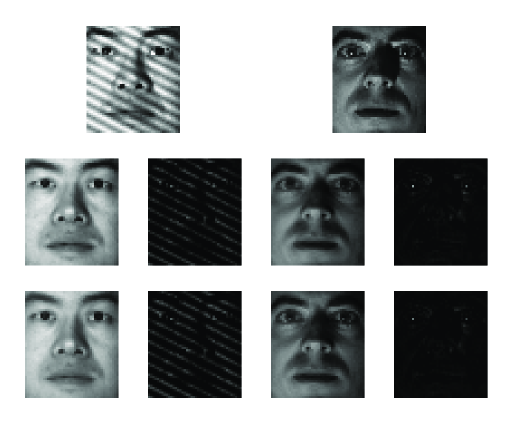
Figure 2: Two examples of using LRR and RSI to correct corruptions in face images in the Extended Yale Database B. The parameters are set as $\lambda_{LRR}=0.05$ and $\lambda_{RSI}=0.6$, respectively. The first row shows two original faces in the database. The second and third rows show the denoising result by LRR and RSI, respectively. For each face, the corrected images are displayed on the left, and the noise images are displayed on the right.

6 Conclusions

We have analyzed LRR and revealed its close relationship with the factorization methods. In particular, we prove that when the data is clean, the LRR problem has a unique solution, which is exactly the shape interaction matrix of the data matrix, and the minimum objective function value is the rank of the data matrix. We further propose the Robust Shape Interaction method, which first removes the noise by column sparse robust PCA, and then computes the SIM of the corrected data for subspace segmentation. RSI is verified by experiments to be more robust than LRR.

References

- [1] Y. Ma, H. Derksen, W. Hong, and J. Wright, “Segmentation of multivariate mixed data via lossy data coding and compression,” IEEE Transactions on Pattern Analysis and Machine Intelligence, pp. 1546–1562, 2007.
- [2] A. Yang, S. Rao, and Y. Ma, “Robust statistical estimation and segmentation of multiple subspaces,” in Computer Vision and Pattern Recognition Workshop on 25 Years on RANSAC, 2006, pp. 99–107.
- [3] J. Costeira and T. Kanade, “A multibody factorization method for independently moving objects,” International Journal of Computer Vision, vol. 29, no. 3, pp. 159–179, 1998.
- [4] A. Gruber and Y. Weiss, “Multibody factorization with uncertainty and missing data using the EM algorithm,” in IEEE Conference on Computer Vision and Pattern Recognition, vol. 1, 2004, pp. 707–714.
- [5] R. Vidal, R. Tron, and R. Hartley, “Multiframe motion segmentation with missing data using powerfactorization and GPCA,” International Journal of Computer Vision, vol. 79, no. 1, pp. 85–105, 2008.
- [6] Y. Ma, A. Yang, H. Derksen, and R. Fossum, “Estimation of subspace arrangements with applications in modeling and segmenting mixed data,” SIAM Review, vol. 50, no. 3, pp. 413–458, 2008.
- [7] E. Elhamifar and R. Vidal, “Sparse subspace clustering,” in IEEE Conference on Computer Vision and Pattern Recognition, vol. 2, 2009, pp. 2790–2797.
- [8] G. Liu, Z. Lin, and Y. Yu, “Robust subspace segmentation by low-rank representation,” in International Conference of Machine Learning, 2010.
- [9] J. Wright, A. Ganesh, S. Rao, and Y. Ma, “Robust principal component analysis: Exact recovery of corrupted low-rank matrices via convex optimization,” submitted to Journal of the ACM, 2009.
- [10] Z. Lin, M. Chen, L. Wu, and Y. Ma, “The augmented Lagrange multiplier method for exact recovery of corrupted low-rank matrix,” submitted to Mathematical Programming, 2009.
- [11] R. Tron and R. Vidal, “A benchmark for the comparison of 3-D motion segmentation algorithms,” in IEEE Conference on Computer Vision and Pattern Recognition, 2007, pp. 1–8.
- [12] K. Lee, J. Ho, and D. Kriegman, “Acquiring linear subspaces for face recognition under variable lighting,” IEEE Transactions on Pattern Analysis and Machine Intelligence, pp. 684–698, 2005.