Renormalization group approach to spinor Bose-Fermi mixtures in a shallow optical lattice

Abstract

We study a mixture of ultracold spin-half fermionic and spin-one bosonic atoms in a shallow optical lattice where the bosons are coupled to the fermions via both density-density and spin-spin interactions. We consider the parameter regime where the bosons are in a superfluid ground state, integrate them out, and obtain an effective action for the fermions. We carry out a renormalization group analysis of this effective fermionic action at low temperatures, show that the presence of the spinor bosons may lead to a separation of Fermi surfaces of the spin-up and spin-down fermions, and investigate the parameter range where this phenomenon occurs. We also calculate the susceptibilities corresponding to the possible superfluid instabilities of the fermions and obtain their possible broken-symmetry ground states at low temperatures and weak interactions.

I Introduction

The remarkable experimental achievements in the field of ultracold atom physics have made it possible to generate mixtures of fermionic atoms with different spin populationspolarized_expmt , as well as mixtures of fermionic and bosonic atoms in a trapbf_expmt1 that can also be loaded on optical latticesbf_expmt2 . Multi-species fermions with unequal densities have also been extensively studied not only in cold atom systems, but also in electronic materials, such as the magnetic-field induced organic superconductorsorganics and other correlated fermion systemselectrons , as well as in the context of color superconductivity in dense quark matterquarks . Bose-Fermi mixtures present a rich phase diagram and have also been subject of intense researchbf_strong ; bf_1d ; bf_phasesep ; bf_staggered ; blatter1 ; sk1 ; hops1 ; mediated1 ; mediated2 ; mediated3 ; mediated4 . Several studies on such mixtures have been restricted to either one-dimensional systemsbf_1d or to cases where the coupling between the bosons and the fermions are weak mediated1 ; mediated2 ; mediated3 . The existence of a supersolid phase in these system in such a weak coupling regime has been predictedblatter1 . Phase separationbf_phasesep and phases with staggered currentsbf_staggered have also been investigated. Some of the other studiesbf_strong , which have looked at the strong coupling regime, have restricted themselves to integer filling factors of bosons and fermions or considered a description of these systems at half filling either by using analytical slave-boson mean-field techniquesk1 or numerical dynamical mean-field theoryhops1 .

An interesting aspect of the study of quantum mixtures is that one species of atoms may mediate interactions among atoms of the other species. In a Bose-Fermi mixture where the bosons form a Bose-Einstein condensate (BEC), quantum fluctuation of the BEC can mediate long-range attractive interaction between the fermionsmediated1 ; mediated2 ; mediated3 . Conversely, in another regime, fermions can be viewed as mediating an effective long-range interaction between the bosonic atomsbf_phasesep . In this work we investigate the problem of partially polarized fermions (unequal spin populations) in the presence of mediated interaction due to quantum fluctuations of a BEC of bosonic atoms. Starting from fermions with equal spin populations, we show that the spin asymmetry of the fermion filling factors can arise due to coupling to a spinor BEC. Spinor boson BEC systems have been studied both experimentallyspinor_expmt and theoretically spinor_theory ; 14 . In particular, the phases and low-energy excitations of such a system is well-known. Here we consider the effect of coupling of these excitations to the fermionic atoms in the mixture.

An important tool for understanding the phases of interacting fermions is the renormalization group (RG) techniqueshankar1 . It has been applied to study the phase diagram of a Bose-Fermi mixture with fermion interactions mediated by fluctuations of the boson BEC, on square and triangular latticesmediated2 . The RG for fermions has also been extended to frequency-dependent interactionsret1 , where retardation effects are importantret2 ; mediated3 . In this work, we use the renormalization group technique to study a mixture of ultracold spin-half fermionic and spin-one bosonic atoms in a shallow optical lattice in two dimensions where the bosons are coupled to the fermions via both density-density and spin-spin interactions. The main aim of our study is to understand the effect of an inter-species on-site SU(2) invariant spin-spin interaction on the phases of this system. We consider the parameter regime where the interaction between the bosons and the fermions are weak and the bosons are in a superfluid state. We then start with a mean-field treatment of the bosons, and include quantum fluctuations to first order within a $1/N$ approximation. After a suitable Bogoliubov transformation, the bosonic modes are integrated out, and an effective action for the fermions is obtained. We find that, when the bosons are in a spinor superfluid state, the spin-spin interaction leads to an effective fermionic action with shifted Fermi surfaces for the up- and down-spin fermions. We then carry out a renormalization group analysis of this effective fermionic action at low temperature and chart out the fate of such a shift under RG flow for different parameter regimes. We also calculate the susceptibilities corresponding to the superfluid instabilities of the fermions and obtain the possible broken-symmetry fermionic ground states at low temperature and weak interactions. In particular we show that the leading instability for the fermions with attractive interaction and circular Fermi surface occurs in the triplet superfluid channel.

The organization of the rest of the paper is as follows. In Sec. II, we introduce the model Hamiltonian for the Bose-Fermi mixture and derive the effective fermionic action. In Sec. III, we obtain the RG equations for the fermionic self energy and interactions from this action. Next, in Sec. IV, we analyze the RG flow of different susceptibilities. Finally, we present a discussion of our main results and conclude in Sec. V.

II Effective Fermionic Hamiltonian

The Hamiltonian of a Bose-Fermi mixture in a shallow ultracold lattice is given by $H=H_{F}+H_{B}+H_{BF}$. The fermionic part of the Hamiltonian $H_{F}$ is given by

$$H_{F} = \sum_{{\bf k}\sigma}(\varepsilon_{{\bf k}}-\mu_{F})\widetilde{f}_{{\bf k}\sigma}^{\dagger}\widetilde{f}_{{\bf k}\sigma}$$ (1)

$$+\sum_{{\bf q},{\bf k},{\bf k}^{\prime},\sigma}U^{1}_{{\bf q}}{\widetilde{f}}^{\dagger}_{{\bf k}^{\prime}-{\bf q},\sigma}\widetilde{f}_{{\bf k}^{\prime},\sigma}\widetilde{f}^{\dagger}_{{\bf k}+{\bf q},\sigma}\widetilde{f}_{{\bf k},\sigma}$$

$$+\sum_{{\bf q},{\bf k},{\bf k}^{\prime},\sigma}U^{2}_{{\bf q}}{\widetilde{f}}^{\dagger}_{{\bf k}^{\prime}-{\bf q},\sigma}\widetilde{f}_{{\bf k}^{\prime},\sigma}\widetilde{f}^{\dagger}_{{\bf k}+{\bf q},{\bar{\sigma}}}\widetilde{f}_{{\bf k},{\bar{\sigma}}},$$

where $\widetilde{f}_{{\bf k}\sigma}(\widetilde{f}_{{\bf k}\sigma}^{\dagger})$ is the annihilation(creation) operator for the fermions, $\mu_{F}$ denotes their bare chemical potential (taken to be independent of the spin of the fermions), $U_{{\bf q}}^{1(2)}$ denotes the bare interaction between the fermions on the same (separate) Fermi surfaces, $\varepsilon_{{\bf k}}=-2t_{F}[\cos(k_{x}a)+\cos(k_{y}a)]$ is the fermion dispersion, $t_{F}$ is the hopping amplitude of the fermions between the neighboring sites, ${\bar{\sigma}}=\downarrow(\uparrow)$ for $\sigma=\uparrow(\downarrow)$, and $a$ is the lattice spacing. For later use, we define the two-component fermionic field $\phi_{i}=(\widetilde{f}_{i\uparrow},\widetilde{f}_{i\downarrow})^{T}$ and use it to represent the fermionic spin-density $S_{i\gamma}^{F}=\phi_{i}^{\dagger}\sigma_{\gamma}\phi_{i}$ and number density $n_{i}^{F}=\phi_{i}^{\dagger}\phi_{i}$, where $\vec{\sigma}=(\sigma_{x},\sigma_{y},\sigma_{z})$ denotes the Pauli matrices.

The Hamiltonian $H_{B}$ for the spinor bosons is given by 14

$$H_{B} = -t_{b}\sum_{<i,j>,\alpha}\widetilde{b}_{i\alpha}^{\dagger}\widetilde{b}_{j\alpha}+\frac{U_{b0}}{2}\sum_{i,\alpha}n_{i\alpha}^{B}(n_{i\alpha}^{B}-1)$$ (2)

$$+ \frac{U_{b2}}{2}\sum_{i,\alpha}(({\bf S}^{B}_{i})^{2}-2n_{i\alpha}^{B})-\mu_{B}\sum_{i,\alpha}n_{i\alpha}^{B},$$

where $\alpha=-1,0,1$ denotes the azimuthal spin quantum number of the bosons, $\widetilde{b}_{i\alpha}$ ($n_{i\alpha}^{B}=\widetilde{b}_{i\alpha}^{\dagger}\widetilde{b}_{i\alpha}$) is the bosonic annihilation (density) operator, $t_{b}$ is the boson hopping amplitude between neighboring sites, $U_{b0}$ and $U_{b2}$ denote the on-site boson interaction strengths in the spin-0 and spin-2 channels respectively, and $\mu_{B}$ is the chemical potential for the bosons. The spin density of these bosons can be expressed in terms of the generators of spin-one matrices: ${\bf S}_{i}^{B}=\widetilde{b}_{i\alpha}^{\dagger}{\bf\lambda}_{\alpha\beta}\widetilde{b}_{i\beta}$. The detailed expression for the generators ${\bf\lambda}$ is given in Appendix A.

The most general SU(2) invariant on-site interaction between the bosons and the fermions is represented by $H_{BF}$. Note that since the fermions carry spin half, conservation of azimuthal quantum number $m_{s}$ does not preclude an on-site spin-spin interaction between the bosons and the fermions. Thus we consider the Hamiltonian $H_{BF}$ to be of the form

$$H_{BF} = U_{ss}\sum_{i}{\bf S}_{i}^{F}\cdot{\bf S}_{i}^{B}+U_{dd}\sum_{i}n_{i}^{F}n_{i}^{B}.$$ (3)

In what follows, we are going to consider the parameter regime $U_{ss}\ll U_{dd}\neq 0$. We note that the presence of a non-zero $U_{ss}$ is a key feature of the subsequent analysis carried out in this work.

Figure 1: Schematic representation of the separation between the up and down spin Fermi surface. $\delta K_{F}=(K_{F\downarrow}-K_{F\uparrow})$ is the difference between the magnitudes of the up and the down spin Fermi momenta.

The analysis of the coupled Bose-Fermi system is most easily done in terms of coherent state path integrals. Following standard prescription, we write the partition function of the system as

$$Z = \int D[b]D[b^{\ast}]D[f]D[f^{\ast}]e^{-S[f,f^{\ast},b,b^{\ast}]},$$

$$S = S_{B}+S_{F}+S_{BF},$$

$$S_{B} = -\frac{1}{\beta}\sum_{\Omega_{n}}\left[\sum_{\bf k}\left[b^{\ast}({\bf k},\Omega_{n})i\Omega_{n}b({\bf k},\Omega_{n})\right]-H_{B}[b^{\ast},b]\right],$$

$$S_{F} = -\frac{1}{\beta}\sum_{\omega_{n}}\left[\sum_{\bf k}\left[f^{\ast}({\bf k},\omega_{n})i\omega_{n}f({\bf k},\omega_{n})\right]-H_{F}[f^{\ast},f]\right],$$

$$S_{BF} = \frac{1}{\beta^{2}}\sum_{\omega_{n},\Omega_{n}}H_{BF},$$ (4)

where $b=(b_{1},b_{0},b_{-1})$ [$f=(f_{\uparrow},f_{\downarrow})$] denotes bosonic [fermionic] fields, $\Omega_{n}$ ($\omega_{n}$) denote bosonic (fermionic) Matsubara frequencies, and $\beta=1/k_{B}T$ with $T$ being the temperature, and $k_{B}$ the Boltzmann constant.

We begin with the analysis of $S_{B}$. We transform the Hamiltonian written in Eq. (2) into $x,y,z$ basis by using the following relations

$${b}_{x}^{*} = \frac{1}{\sqrt{2}}({b}_{-1}^{*}-{b}_{1}^{*})\ ,$$

$${b}_{y}^{*} = \frac{i}{\sqrt{2}}({b}_{-1}^{*}+{b}_{1}^{*})\ ,$$

$${b}_{z}^{*} = {b}_{0}^{*}.$$ (5)

We assume that the bosonic spinor system is deep in the BEC state. The standard procedure for analyzing such a BEC involves expressing the bosonic field $b$ as

$${b}_{\alpha}({\bf q},i\Omega_{n}) = \Psi_{0\alpha}\delta_{{\bf q},0}+{a}_{\alpha}({\bf q},i\Omega_{n}),$$ (6)

where $\Psi_{0\alpha}=\langle{b}_{\alpha}({\bf q}=0,\Omega_{n}=0)\rangle$, and expanding $S_{B}$ to order $O(a_{\alpha}^{2})$. The mean-field equation for the condensate is then obtained by imposing the coefficient of $a_{0}$ and $a_{0}^{\dagger}$ to be zero. This analysis yields

$$\Psi_{0\alpha}^{*}\left[-4t_{b}+\left(n_{0}-\frac{1}{2}\right)U_{b0}+(n_{0}-1)U_{b2}-\mu_{b}\right]$$

$$-\frac{U_{b2}}{N}\sum_{\beta\neq\alpha}(\Psi_{0\beta}^{*})^{2}\Psi_{0\alpha}=0,$$ (7)

where we have introduced the condensate density $n_{0}=N_{b}/N$, with $N_{b}$ being the total number of bosons in the system, and $N$ the total number of lattice sites. As shown in a previous study, Eq. (7) supports two solutions14 . The first is a ferromagnetic phase with

$$\Psi_{\rm ferro}=\sqrt{n_{0}N/2}(1,\pm i,0)^{T},$$ (8)

while the other is a polar phase with $\Psi_{\rm polar}=\sqrt{n_{0}N}(1,0,0)^{T}$. The ferromagnetic state becomes energetically favorable for $U_{b2}<0$ and in the rest of the paper we concentrate on this regime and work with the solution $\Psi_{\rm ferro}=\sqrt{n_{0}N/2}(1,i,0)^{T}$ which corresponds to $\langle b_{1}\rangle\neq 0$. The choice of one of the these two solutions can be easily seen to be the effect of any stray magnetic field that might be present in a realistic experimental system. We note that for the polar phase, the low-energy physics of the Bose-Fermi mixture is identical to its counterpart with spinless bosons mediated2 ; mediated3 .

A detailed analysis of $S_{B}$ when the bosons are in the ferromagnetic phase is carried out in Appendix A and leads to the expression for $S_{B}$ [Eq. (30)] which is quadratic in the fluctuation fields $a_{\alpha}({\bf q},i\Omega_{n})$. Thus, using Eq. (30) and Eq. (3), one can integrate out the boson degrees of freedom and obtain, after a straightforward but tedious calculation, an effective action for the fermions,

$$S_{\rm eff} = -\frac{1}{\beta}\sum_{i\omega_{n}}\Big{[}\sum_{{\bf k}}f^{\ast}_{{\bf k},\sigma}[i\omega_{n}-\varepsilon_{{\bf k}}+\mu_{F\sigma}]f_{{\bf k},\sigma}$$ (9)

$$-\sum_{{\bf k,k^{\prime},q},\sigma}\widetilde{U}_{{\bf q},\sigma\sigma}f^{\ast}_{{\bf k}+{\bf q},\sigma}f_{{\bf k},\sigma}f^{\ast}_{{\bf k^{\prime}-q},\sigma}f_{{\bf k^{\prime}},\sigma}$$

$$-\sum_{{\bf k,k^{\prime},q}}\widetilde{U}_{{\bf q},\uparrow\downarrow}f^{\ast}_{{\bf k+q},\uparrow}f_{{\bf k},\downarrow}f^{\ast}_{{\bf k^{\prime}-q},\downarrow}f_{{\bf k^{\prime}},\uparrow}\Big{]}\ ,$$

where $\mu_{F\sigma}=\mu_{F}-[n_{0}U_{ss}({\rm Sgn}\sigma)+U_{dd}n_{0}]$, and ${\rm Sgn}\sigma=1(-1)$ for $\sigma=\uparrow(\downarrow)$. Thus the spin-spin interaction between the bosons and the fermions leads to an effective shift between the spin-up and spin-down Fermi surfaces, as shown in Fig. 1 , at the mean-field level. The sign of the shift depends on the choice of one of the two solutions given by Eq. 8; for our choice $\Psi_{\rm ferro}=\sqrt{n_{0}N/2}(1,i,0)^{T}$, the down-spin Fermi surface is enhanced compared to the up-spin one as shown in Fig. 1. The effective interactions $\widetilde{U}_{{\bf q},\sigma\sigma}$ and $\widetilde{U}_{{\bf q},\uparrow\downarrow}$ are given by

$$\widetilde{U}_{{\bf q},\sigma\sigma} = U_{\bf q}^{1}-\frac{n_{0}}{2}(U_{dd}+({\rm Sgn}\sigma)U_{ss})^{2}\chi_{{\bf q},\sigma\sigma},$$ (10)

$$\widetilde{U}_{{\bf q},\uparrow\downarrow} = U_{\bf q}^{2}+\frac{n_{0}}{2}(U_{dd}^{2}-U_{ss}^{2})\chi_{{\bf q},\uparrow\downarrow},$$ (11)

where

$$\chi_{q,\sigma\sigma^{\prime}}=\frac{\xi_{{\bf q},\sigma\sigma^{\prime}}-2U_{b2}n_{0}}{(\xi_{{\bf q},\sigma\sigma^{\prime}}-2U_{b2}n_{0})^{2}+\Omega_{n}^{2}},$$ (12)

and $\xi_{{\bf q},\sigma\sigma^{\prime}}=-2t_{b}[\cos(q_{x\sigma\sigma^{\prime}})+\cos(q_{y\sigma\sigma^{\prime}})-2]$ is the boson dispersion at the wave-vector $q_{x[y]\sigma\sigma}=K_{F\sigma}\cos(\theta)[\sin(\theta)]$, $q_{x[y]\sigma{\bar{\sigma}}}=(K_{F\sigma}+K_{F{\bar{\sigma}}})\cos(\theta)[\sin(\theta)]/2$. Here we have set the lattice spacing $a=1$, $K_{F\sigma}$ is the magnitude of the Fermi wave-vector for electrons with spin $\sigma$, and we have restricted ourselves to the regime where $|K_{F\uparrow}-K_{F\downarrow}|\ll K_{F\uparrow},K_{F\downarrow}$. This restricts the validity of our analysis to the parameter regime $\mu_{F}\gg U_{ss}$. Note that ${\widetilde{U}}_{{\bf q},\uparrow\downarrow}$ represents the amplitude of scattering between fermions on separate Fermi surfaces, while scattering processes represented by ${\widetilde{U}}_{{\bf q},\sigma\sigma}$ involve fermions on the same Fermi surface. For the rest of the paper, we shall ignore the retardation effects of the effective interaction and shall thus set $\Omega_{n}=0$ and restrict ourselves to circular Fermi surfaces with small effective shifts between them (as shown in Fig. 1).

Next, following standard procedure outlined in Ref. shankar1, , we antisymmetrize $\widetilde{U}_{{\bf q},\sigma\sigma}$ with respect to the interchange ${\bf k_{1}}\leftrightarrow{\bf k_{2}}$ and ${\bf k_{3}}\leftrightarrow{\bf k_{4}}$ (where, ${\bf k_{1}}={\bf k^{\prime}},~{}{\bf k_{2}}={\bf k},~{}{\bf k_{3}}={\bf k^{\prime}-q},~{}{\bf k_{4}}={\bf k+q}$). Further, following Ref. shankar1, and using the circular nature of the Fermi surface, we consider fermion scattering only in the forward (${\bf k_{1}}={\bf k_{4}}$ and ${\bf k_{2}}={\bf k_{3}})$ and BCS (${\bf k_{2}}=-{\bf k_{1}}$ and ${\bf k_{4}}=-{\bf k_{3}}$) channels. The contribution of $\widetilde{U}_{{\bf q},\sigma\sigma}$ to these channels can be computed from Eqs. (11) and (12). Denoting interaction couplings in these channels by $\widetilde{F}_{\sigma\sigma}(\theta_{12})$ and $\widetilde{V}_{\sigma\sigma}(\theta_{13})$, respectively, we find that

$$\widetilde{F}_{\sigma\sigma}(\theta_{12}) = \left[U_{0}-n_{0}\left(\frac{U_{dd}+({\rm Sgn}\sigma)U_{ss}}{2n_{0}U_{b2}}\right)^{2}K_{F\sigma}^{2}\right]$$ (13)

$$\times[1-\cos(\theta_{12})],$$

$$\widetilde{V}_{\sigma\sigma}(\theta_{13}) = \left[U_{0}-n_{0}\left(\frac{U_{dd}+({\rm Sgn}\sigma)U_{ss}}{2n_{0}U_{b2}}\right)^{2}K_{F\sigma}^{2}\right]$$ (14)

$$\times\cos(\theta_{13}),$$

where, $\theta_{12}(\theta_{13})$ is the angle between ${\bf k_{1}}$ and ${\bf k_{2}}({\bf k}_{3})$, $U_{0}(1-\cos(\theta_{12}))[U_{0}\cos(\theta_{13})]$ denote the value of $U_{\bf q}^{1}$ for the forward[BCS] channels. Note that in obtaining Eq. (13) and (14), we have explicitly antisymmetrized the contribution of $\chi_{{\bf q},\sigma\sigma}$ in Eq. (10).

The contributions of $\widetilde{U}_{{\bf q},\uparrow\downarrow}$ in the forward and the BCS channels can also be computed in a similar manner and are given by

$$\widetilde{F}_{\uparrow\downarrow}(\theta_{12}) = \frac{n_{0}(U_{dd}^{2}-U^{2}_{ss})}{4K^{2}_{F,\uparrow\downarrow}(1-{\cos}(\theta_{12}))-4n_{0}U_{b2}},$$

$$\widetilde{V}_{\uparrow\downarrow}(\theta_{13}) = \frac{n_{0}(U_{dd}^{2}-U^{2}_{ss})}{4K^{2}_{F,\uparrow\downarrow}\cos(\theta_{13})-4n_{0}U_{b2}},$$ (15)

where, $K_{F,\uparrow\downarrow}=(K_{F\uparrow}+K_{F\downarrow})/2$ and we have set the contribution of $U_{{\bf q}}^{2}$ to the forward and BCS channels to zero. We have checked explicitly that finite value of $U_{\bf q}^{2}$ does not alter the qualitative conclusions of the work.

III RG equations for self-energy and couplings

In this section, we carry out a RG analysis of $S_{\rm eff}$ adapting one-loop Wilsonian RG using a path integral approach. The details of this approach are outlined in several past works shankar1 ; ret1 ; ret2 . The key idea behind such a procedure is to consider $S_{\rm eff}$ as the starting fermionic action at a high-energy cutoff scale $\Lambda$, perform Wilson RG on this action and derive the flow equations for the effective interactions and fermionic self-energy. It is well known shankar1 that for a circular Fermi surface as considered here, only the interaction in the BCS channels ($V$) flow under RG and that the key contribution to the fermionic self-energy within one-loop RG comes from the forward channels ($F$).

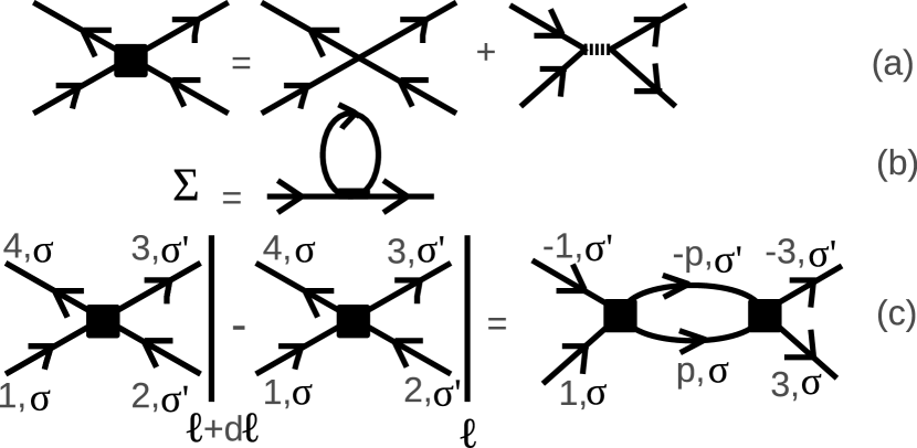
Figure 2: (a) Schematic representation of the effective fermionic interaction $\widetilde{U}$ (left) as sum of the bare interaction $U_{0}$ and the contribution from the bosons. (b) Diagrammatic representation of the RG flow equation for the self-energy ($\Sigma_{\sigma}$) correction which receives contribution from the interaction in the forward channel $F$. (c) Diagrammatic representation for the RG flow equations for $V$. We use the simplified notation $1={\bf k^{\prime}}$, 2=${\bf k}$, $3={\bf k}^{\prime}-{\bf q}$, $4={\bf k}+{\bf q}$, and $\sigma$ and $\sigma^{\prime}$ takes values $\uparrow$ and $\downarrow$.

Using these facts, the relevant diagrams for the contribution to the self-energy and the effective interactions in the present model [Eq. (9)] can be easily found. These are shown in Fig. 2. The RG equations for the interactions and the fermionic self-energy, as obtained from these diagram in Fig. 2, are given by,

$$\frac{d\Sigma_{\sigma}(\theta)}{d\ell} = -\frac{1}{2\pi}\int_{\theta^{\prime}\omega_{n}}\Big{(}K_{F\sigma}\widetilde{F}_{\sigma\sigma}(\theta^{\prime}-\theta)G_{\sigma}(\omega_{n},\theta^{\prime})$$ (16)

$$+K_{F{\bar{\sigma}}}\widetilde{F}_{\uparrow\downarrow}(\theta^{\prime}-\theta)G_{\bar{\sigma}}(\omega_{n},\theta^{\prime})\Big{)},$$

$$\frac{d\widetilde{V}_{\sigma\sigma}(\theta_{1}-\theta_{3})}{d\ell} = -\frac{K_{F\sigma}}{2\pi}\int_{\theta\omega_{n}}\widetilde{V}_{\sigma\sigma}(\theta_{1}-\theta)\widetilde{V}_{\sigma\sigma}(\theta-\theta_{3})$$ (17)

$$\times G_{\sigma}(\omega_{n},\theta)G_{\sigma}(-\omega_{n},\theta+\pi),$$

$$\frac{d\widetilde{V}_{\uparrow\downarrow}(\theta_{1}-\theta_{3})}{d\ell} = -\frac{K_{F\uparrow\downarrow}}{2\pi}\int_{\theta\omega_{n}}\widetilde{V}_{\uparrow\downarrow}(\theta_{1}-\theta)\widetilde{V}_{\uparrow\downarrow}(\theta-\theta_{3})$$ (18)

$$\times G_{\downarrow}(\omega_{n},\theta)G_{\uparrow}(-\omega_{n},\theta+\pi),$$

where we have carried out the integrals over the radial momentum perpendicular to the circular Fermi surface, $\Lambda=\Lambda_{0}e^{-\ell}$ is the RG cutoff, $\Lambda_{0}<E_{F}$ is the cut-off in the beginning of the RG flow, ${\ell}$ is the RG time, $\int_{\theta^{\prime}\omega_{n}}=1/\beta\sum_{i\omega_{n}}\int d\theta^{\prime}/(2\pi)$ denotes frequency sum and integral over transverse momenta over the Fermi surface, $\Sigma_{\sigma}(\theta)$ denotes the self-energy for fermions with spin $\sigma$ and momentum ${\bf k}=(K_{F\sigma}\cos(\theta),K_{F\sigma}\sin(\theta))$, $K_{F,\sigma\overline{\sigma}}=(K_{F\uparrow}+K_{F\downarrow})/2$, $\epsilon_{\sigma}(\theta^{\prime})$ is the fermion dispersion on the Fermi surface with spin $\sigma$ , and the fermion Green function, evaluated on the Fermi surface for spin $\sigma$ electrons are given by

$$G_{\sigma}(\omega_{n},\theta)=\left(i\omega_{n}-(\epsilon_{\sigma}(\theta)-\mu_{\sigma})-\Sigma_{\sigma}(\theta)\right)^{-1}.$$ (19)

Before solving Eqs. (16)..(18) numerically, we note that $\epsilon_{\sigma}(\theta)=-2t[\cos(K_{F\sigma}\cos(\theta))+\cos(K_{F\sigma}\sin(\theta))]$ have a very weak $\theta$ dependence. Further, the integration $\widetilde{F}_{\sigma\sigma^{\prime}}(\theta^{\prime}-\theta)$ over $\theta^{\prime}$ for a complete cycle renders it independent of $\theta$ as well. Consequently, $\Sigma_{\sigma}$ becomes independent of $\theta$. Thus, at low temperature, $\sum_{\omega_{n}}G_{\sigma}(\omega_{n},\theta)G_{\sigma^{\prime}}(-\omega_{n},\theta+\pi)$ becomes practically independent of $\theta$. Using this fact, it is possible to express Eqs. (16)..(18) in the angular momentum channels denoted by $l$ to obtain

$$\frac{d\Sigma_{\sigma}^{l}}{d\ell} = -\frac{1}{2\pi}\Big{(}K_{F\sigma}\widetilde{F}_{\sigma\sigma}^{l}G_{\sigma}^{l}+K_{F{\bar{\sigma}}}\widetilde{F}_{\uparrow\downarrow}^{l}G_{\bar{\sigma}}^{l}\Big{)},$$ (22)

$$\frac{d\widetilde{V}_{\sigma\sigma}^{l}}{d\ell}\simeq-\frac{K_{F\sigma}J_{\sigma\sigma}}{2\pi}(\widetilde{V}_{\sigma\sigma}^{l})^{2},$$

$$\frac{d\widetilde{V}_{\uparrow\downarrow}^{l}}{d\ell}\simeq-\frac{K_{F\uparrow\downarrow}J_{\uparrow\downarrow}}{2\pi}(\widetilde{V}_{\uparrow\downarrow}^{l})^{2}.$$

where $\widetilde{V}_{\sigma\sigma^{\prime}}^{l}[\widetilde{F}_{\sigma\sigma^{\prime}}^{l}]$ and $G^{l}_{\sigma}$ are given by

$$\widetilde{V}_{\sigma\sigma^{\prime}}^{l}[\widetilde{F}_{\sigma\sigma^{\prime}}^{l}] = \int_{0}^{2\pi}\frac{d\theta}{2\pi}e^{il\theta}\widetilde{V}_{\sigma\sigma^{\prime}}(\theta)[\widetilde{F}_{\sigma\sigma^{\prime}}^{l}(\theta)],$$ (23)

$$G_{\sigma}^{l} = \int_{0}^{2\pi}\frac{d\theta}{2\pi}e^{il\theta}(1/\beta\sum_{i\omega_{n}}G_{\sigma}(\omega_{n},\theta)),$$

$$J_{\sigma\sigma} = \frac{1}{\beta}\sum_{i\omega_{n}}G_{\sigma}(\omega_{n},\theta)G_{\sigma}(-\omega_{n},\theta+\pi),$$

$$J_{\uparrow\downarrow} = \frac{1}{\beta}\sum_{i\omega_{n}}G_{\uparrow}(\omega_{n},\theta)G_{\downarrow}(-\omega_{n},\theta+\pi).$$ (24)

Next, we solve the RG equations for self energy and couplings numerically for a temperature $\beta t_{F}=10$. We have carried out the numerical solution of both Eqs. (16)..(18) and Eqs. (22)..(22) and checked that these yield identical results confirming our observation on the absence of $\theta$ dependence of $J_{\sigma\sigma}$ and $J_{\uparrow\downarrow}$. For the numerical solution of these equations, we have scaled all the energy parameters in units of $2t_{F}$. We note that at the one-loop level, the effect of $\Sigma_{\sigma}$ is to renormalize the chemical potential $\mu_{F\sigma}$ and hence their difference: $\delta\mu=|\mu_{F\uparrow}-\mu_{F\downarrow}+\Sigma^{l}_{\uparrow}-\Sigma^{l}_{\downarrow}|=|\delta\mu_{int}+\Sigma^{l}_{\uparrow}-\Sigma^{l}_{\downarrow}|$, where $\delta\mu_{int}=\mu_{F\uparrow}-\mu_{F\downarrow}=-2n_{0}U_{ss}$. In Figs. 3 and 4, we show the variation of $\delta\mu$ as a function of the RG time $\ell$ for $U_{0}=\pm 0.3$, $n_{0}=0.9$, $U_{b2}=-0.08$ and three different representative values of $\delta\mu_{int}$. We find that the RG flow is essentially controlled by the induced interaction part of $F_{\sigma\sigma^{\prime}}$ and displays little dependence on $U_{0}$. The separation between the Fermi surfaces is always amplified and the spin-up and spin-down Fermi surfaces flow away from each other. This signifies a possibility of either a Ferromagnetic or triplet superfluid (with equal-spin pairing) instabilities of the system. Note that such instabilities, in case they occur, have their root in the initial separation of the opposite spin Fermi surfaces and hence can be attributed to the spin-spin coupling between the fermions and the spinor bosons.

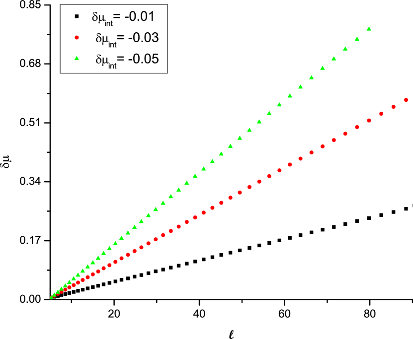
Figure 3: Plot of $\delta\mu~{}{\rm versus}~{}\ell$, for $l=0$, $n_{0}=0.9$, $U_{b2}=-0.08$, $U_{0}=-0.3$ for several values of $\delta\mu_{\rm int}=-0.05$ (green line with triangles), $\delta\mu_{int}=-0.03$ (red line with circles) and $\delta\mu_{int}=-0.01$ (black line with squares).

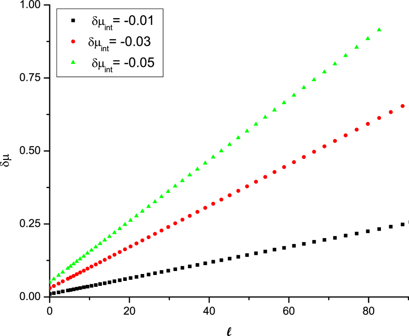
Figure 4: Same as in Fig. 3 but with $U_{0}=$0.3.

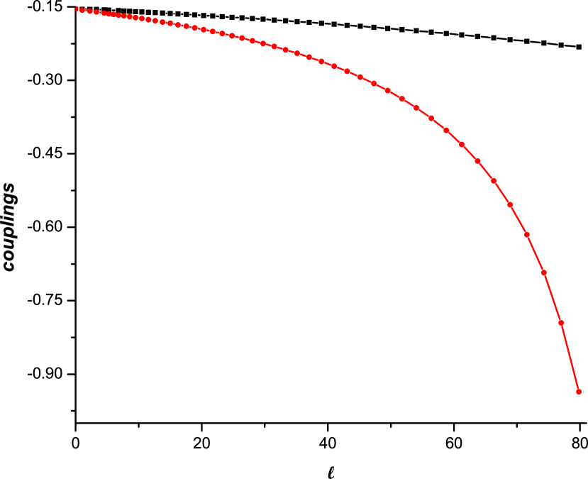
Figure 5: RG flow of the couplings $\widetilde{V}_{\uparrow\uparrow}$ (black line with squares), $\widetilde{V}_{\downarrow\downarrow}$ (red line with circles) for $l=\pm 1$, $U_{0}$= -0.3, $U_{b2}=-0.08$, $\delta\mu_{int}=-0.05$, and $n_{0}=0.9$.

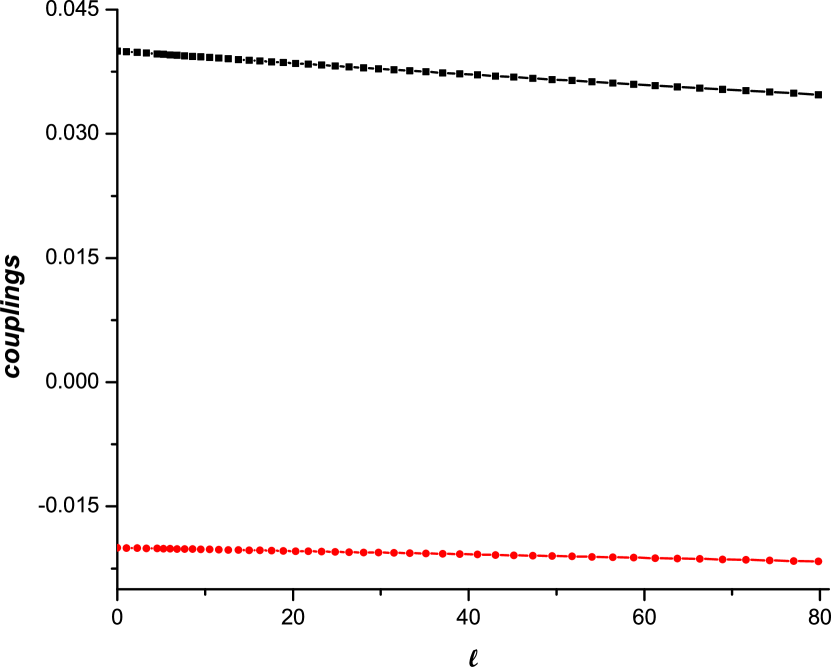
Figure 6: RG flow of the coupling $\widetilde{V}_{\uparrow\downarrow}$ (black line with squares for l=0), $\widetilde{V}_{\uparrow\downarrow}$ (red line with circles for $l=\pm 1$) for $U_{0}$= -0.3, $U_{b2}=-0.08$, $\delta\mu_{int}=-0.05$, and $n_{0}=0.9$.

Next we plot the variation of the couplings with the RG cutoff $\ell$ in Fig. 5 and Fig. 6 for $\delta\mu_{int}=-0.05$, $n_{0}=0.9$, $U_{b2}=-0.08$ and $U_{0}=-0.3$. We find that $\widetilde{V}_{\uparrow\downarrow}$ does not flow appreciably under RG which is a consequence of lack of scattering between Fermi surfaces with opposite spins. The flow of $\widetilde{V}_{\sigma\sigma}$ shows an increase of their magnitude indicating a flow toward strong coupling regime which can not be accessed by our perturbative RG analysis.

IV RG flow of the susceptibilities

In this section, we consider the RG flow for the possible instabilities of the fermionic models. In particular, we consider the singlet and equal-spin paired triplet superfluid (SSF and TSF) instabilities 8 of the metallic phase of the fermions due to the induced interaction. This choice is motivated by the fact that for circular Fermi surfaces considered here we do not have nesting and hence do not expect to have instabilities in the $2k_{F}$ spin- or charge-density wave channels. It is well known that the onset of such instabilities are signalled by the divergence of the corresponding static susceptibilities under RG flow17 .

The flow equations for the static susceptibilities can be derived using standard techniques as elaborated in Refs. 17, ; ret2, ; mediated3, . As outlined in these works, the response function can be calculated by introducing a source term in the action

$$S_{h}=-\sum_{q}h^{\delta}\Delta^{\delta},$$ (25)

where $\delta$ takes values SSF or TSF corresponding to the singlet or equal-spin triplet pairings.

$$\Delta^{{\rm SSF}} = \sum_{\sigma,{\bf k}}(\rm{sgn}\sigma)f_{\sigma}({\bf k})f_{\bar{\sigma}}({\bf-k})~{}~{}~{}{\rm and}$$

$$\Delta^{{\rm TSF}} = f_{\sigma}({\bf k})f_{\sigma}({\bf-k}),$$ (26)

are the order parameters for singlet and triplet superfluidity respectively and $h^{\delta}$ is the external field of type $\delta$. The corresponding response function is given by

$$\chi^{\delta} = \langle{\Delta^{\delta}}^{*}\Delta^{\delta}\rangle=\frac{\delta^{(2)}\rm{ln}Z[h]}{\delta{h^{\delta}}^{*}\delta h^{\delta}}\Big{|}_{h=0},$$ (27)

where $Z[h]$ denotes the partition function in presence of the source term. The RG process generates correction to the source field $h$ along with the higher order terms in the source field. At any RG time $\ell$, the total action $S_{\ell}$ can be written as

$$S_{\ell} = S_{\ell}^{0}-\int dt\,\left[z^{\delta}h^{\delta}\Delta^{\delta}-{h^{\delta}}^{*}h({\bf q})\chi^{\delta}\right],$$ (28)

where $S^{0}_{\ell}$ is the action at RG time $\ell$ without the external field $h$ and the coefficient $z^{\delta}$ is the effective vertex of type $\delta$.

The relevant one-loop diagrams representing the RG equations for the vertices $z^{\delta}$ and the susceptibilities $\chi^{\delta}$ are schematically shown in Fig. 7. The corresponding one-loop flow equations for $z^{\delta}$ and $\chi^{\delta}$ are given by

$$\frac{dz^{\rm{TSF}}_{l,\sigma\sigma}}{d\ell} = -\frac{K_{F\sigma}}{2\pi}J_{\sigma\sigma}\widetilde{V}_{\sigma\sigma}^{l}z^{\rm{TSF}}_{l,\sigma\sigma},$$

$$\frac{d\chi^{\rm{TSF}}_{l,\sigma\sigma}}{d\ell} = \frac{K_{F\sigma}}{2\pi}J_{\sigma\sigma}(z^{\rm{TSF}}_{l,\sigma\sigma})^{2},$$

$$\frac{dz^{\rm{SSF}}_{l}}{d\ell} = -z^{\rm{SSF}}_{l}\sum_{\sigma}\frac{K_{F,\sigma\bar{\sigma}}}{2\pi}({\rm sgn}\sigma)J_{\sigma\bar{\sigma}}\widetilde{V}_{\sigma\bar{\sigma}}^{l},$$

$$\frac{d\chi^{\rm{SSF}}_{l}}{d\ell} = (z^{\rm{SSF}}_{l})^{2}\sum_{\sigma}\frac{K_{F,\sigma\bar{\sigma}}}{2\pi}J_{\sigma\bar{\sigma}},$$ (29)

where we have used the $\theta$ independence of $J_{\sigma\sigma}$ and $J_{\uparrow\downarrow}$. We solve these equations numerically for $\beta t_{F}=10$. The results are shown in Fig. 8 for $U_{0}=-0.3$ for SSF and TSF instabilities. We find that the $\chi_{l,\downarrow\downarrow}^{{\rm TSF}}$ instability shows a divergence around $\ell\simeq 80$ indicating an instability of the metallic ground states against triplet down-spin pairing superfluid ground state. This is an expected consequence of the growing separation of the Fermi surfaces which prevents opposite spin SSF pairing and hence favors down-spin TSF state. Thus we conclude that the most dominant instability of the Fermi superfluid with an attractive interaction is TSF with down-spin pairing. We note that our RG analysis can not predict the subsequent fate of the system once the superfluid instability has set in. The system may either end up with a spin-up metallic Fermi surface coexisting with a triplet superfluid of spin-down fermions or the superfluidity in the spin-down channel may induce a superfluid instability for the spin-up fermions via a momentum-space proximity effect. The latter effect is somewhat similar to that seen for multi-band ruthenate superconductors rice1 . We leave a more thorough analysis of these possibilities as a subject of future study.

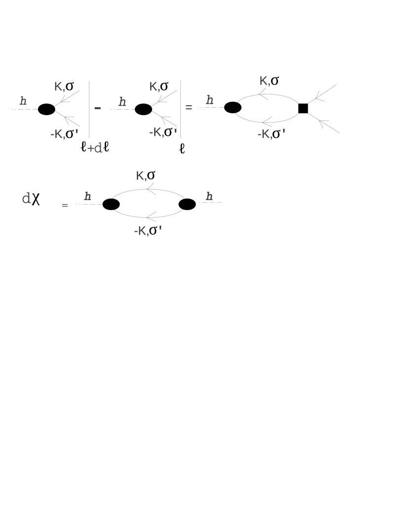
Figure 7: Diagrammatic representation of the renormalization of vertices and the susceptibilities in the BCS channel.

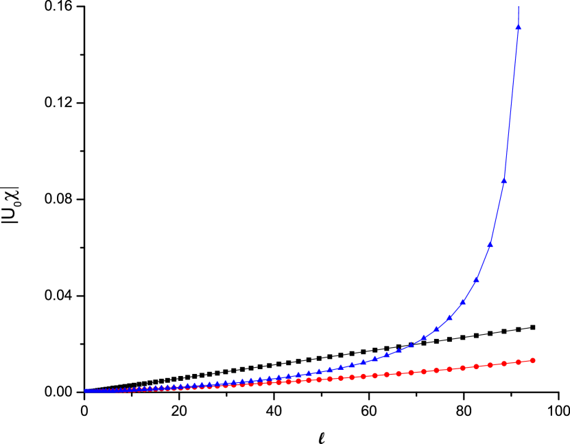
Figure 8: RG flow for the static susceptibilities for $U_{0}=-0.3$. The blue line with triangle and the black line with square indicate RG flow of the susceptibilities for the triplet BCS channels $\chi_{l,\downarrow\downarrow}^{{\rm TSF}}~{}(l=\pm 1)$ and $\chi_{l,\uparrow\uparrow}^{{\rm TSF}}~{}(l=\pm 1)$ respectively. The red line with circle indicates RG flow of the susceptibility for the singlet BCS channel $\chi_{l}^{{\rm SSF}}~{}(l=0)$.

V Conclusion

In conclusion, we have studied a mixture of spinor boson and fermion in a shallow 2D optical lattice using RG and have shown that the presence of an on-site spin-spin interaction between the bosons and the fermions leads to a separation of Fermi surface of the spin-up and spin-down fermions irrespective of the nature of the bare interaction between the fermions provided that the bosons are in the spinor condensate state. Such a separation, depending on the density of the fermions, may give rise to a net spin polarization for the Fermi superfluid. Further, for attractive interaction between these fermions, we have shown that the leading instability of the metallic state of the fermions lies in the TSF channel with down spin pairing. In particular, we predict that for fermions coupled to a spinor bosonic condensate in its ferromagnetic phase via a spin-spin interactions, attractive interactions will induce a down-spin triplet pairing superfluid instability over the otherwise more common singlet pairing instability. We note that this phenomenon is in contrast to the fermions coupled to either a spinless boson condensate or a spinor boson condensate in its polar phase.

VI Acknowledgements

It is our pleasure to thank Filippos Klironomos for invaluable discussions. SWT gratefully acknowledges support from NSF under grant DMR-0847801 and from the UC-Lab FRP under award number 09-LR-05-118602. KS thanks DST, India for support through grant SR/S2/CMP-001/2009.

Appendix A Effective Quadratic Hamiltonian for spinor boson

The generators $\lambda_{+}$, $\lambda_{-}$ for spin-one bosons can be obtained from the spin-rotation matrices in $x$,$y$ and $z$ basis. In this basis we have

$S_{x}=\frac{1}{\sqrt{2}}\left(\begin{array}[]{ccc}0&1&0\\ 1&0&1\\ 0&1&0\end{array}\right)$ , $S_{y}=\frac{1}{\sqrt{2}}\left(\begin{array}[]{ccc}0&-i&0\\ i&0&-i\\ 0&i&0\end{array}\right)$ ,

and $S_{z}=\left(\begin{array}[]{ccc}1&0&0\\ 0&0&0\\ 0&0&-1\end{array}\right)$.

This yields, using $\lambda_{\pm}=S_{x}\pm iS_{y}$
$\lambda_{+}=\left(\begin{array}[]{ccc}0&\sqrt{2}&0\\ 0&0&\sqrt{2}\\ 0&0&0\end{array}\right)$ , $\lambda_{-}=\left(\begin{array}[]{ccc}0&0&0\\ \sqrt{2}&0&0\\ 0&\sqrt{2}&0\end{array}\right),$

and $\lambda_{z}=S_{z}$.

The action $S_{B}$ when the bosons are in the ferromagnetic phase can be written using Ref. 2 and 4 as

$$S_{B} = -\frac{1}{\beta}\sum_{\omega_{n}}\Big{[}\sum_{{\bf k}}[a^{*}_{\alpha}({{\bf k},\Omega_{n})}i\Omega_{n}a_{\alpha}({\bf k},\Omega_{n})$$ (30)

$$-H^{\prime}_{B}[a^{*},a]\Big{]}.$$

$H^{\prime}_{B}$ is the quadratic Hamiltonian for spinor boson in ferromagnetic phase and given by,

$$H^{\prime}_{B}=-\frac{n_{0}^{2}}{2}(U_{b0}+U_{b2})N+\sum_{k,\alpha}[\xi_{k}+\frac{n_{0}}{2}(1-\delta_{\alpha z})(U_{b0}-U_{b2})]a_{k\alpha}^{\dagger}a_{k\alpha}-\frac{n_{0}}{2}(U_{b0}+3U_{b2})\sum_{k}i(a_{kx}^{\dagger}a_{ky}-a_{ky}^{\dagger}a_{kx})$$

$$+\frac{n_{0}}{4}(U_{b0}+U_{b2})\sum_{k}(a_{kx}a_{-kx}+a_{kx}^{\dagger}a_{-kx}^{\dagger}-a_{ky}a_{-ky}-a_{ky}^{\dagger}a_{-ky}^{\dagger})+\frac{n_{0}}{2}(U_{b0}+U_{b2})\sum_{k}i(a_{kx}^{\dagger}a_{-ky}^{\dagger}-a_{kx}a_{-ky}),$$ (31)

where , $\xi_{k}=\varepsilon_{k}+4t_{b}=-2t_{b}({\rm cos}(k_{x}a)+{\rm cos}(k_{y}a)-2)$. We then decouple the boson fields using Eq. (7) and expand about the ferromagnetic condensate saddle point to obtain the quadratic effective action for the bosons. This action has the form

$$S_{B}^{\rm eff} = -\frac{1}{\beta}\sum_{\omega_{n}}\sum_{{\bf k}}{\mathcal{A}}^{\ast}({\bf k},\Omega_{n})G_{B}^{-1}{\mathcal{A}}({\bf k},\Omega_{n}),$$ (32)

where ${\mathcal{A}}({\bf k},\Omega_{n})$ denotes the fluctuating boson fields given by

$${\mathcal{A}}^{\ast}({\bf k},\Omega_{n}) = \left[a^{*}_{x}({\bf k},\Omega_{n}),a_{x}(-{\bf k},\Omega_{n}),a^{*}_{y}({\bf k},\Omega_{n}),\right.$$

$$\left.a_{y}(-{\bf k},\Omega_{n}),a^{*}_{z}({\bf k},\Omega_{n}),a_{z}(-{\bf k},\Omega_{n})\right],$$

and $G_{B}^{-1}$ denotes the boson Green’s function given by

$$G_{B}^{-1}=-\left(\begin{array}[]{cccccc}P_{{\bf k}-}&A&-iB&iA&0&0\\ A&P_{{\bf k}+}&-iA&iB&0&0\\ iB&iA&P_{{\bf k}-}&-A&0&0\\ -iA&-iB&-A&P_{{\bf k}+}&0&0\\ 0&0&0&0&\xi_{{\bf k}-}&0\\ 0&0&0&0&0&\xi_{{\bf k}+}\end{array}\right),$$ (40)

where, $P_{{\bf k}\pm}=\xi_{{\bf k}}+\frac{n_{0}}{2}(U_{b0}-U_{b2})\pm i\Omega_{n}$ , $\xi_{{\bf k}\pm}=\xi_{{\bf k}}\pm i\Omega_{n}$, $A=\frac{n_{0}}{2}(U_{b0}+U_{b2})$ and $B=\frac{n_{0}}{2}(U_{b0}+3U_{b2})$. Using Eq. (30) and Eq. (3), we integrate out the bosons by following standard technique and obtain effective fermionic action as written in Eq. (9) .

References

- (1) M. W. Zwierlein, A. Schirotzek, C. H. Schunck, and W. Ketterle, Science 311, 492 (2006); G. B. Partridge, W. Li, R. I. Kamar, Y.-A. Liao, R. G. Hulet, Science 311, 503 (2006); Y. Shin, M. W. Zwierlein, C. H. Schunck, A. Schirotzek, W. Ketterle, Phys. Rev. Lett. 97, 030401 (2006); G. B. Partridge, W. Li, Y.-A. Liao, R. G. Hulet, M. Haque, and H. T. C. Stoof, Phys. Rev. Lett. 97, 190407 (2006); Y. Liao, A. S. C. Rittner, T. Paprotta, W. Li, G. B. Partridge, R. G. Hulet, S. K. Baur, and E. J. Mueller, Nature 467, 567 (2010).
- (2) G. Modugno, G. Roati, F. Riboli, F. Ferlaino, R. J. Brecha, and M. Inguscio, Science 297, 2240 (2002); J. Goldwin, S. Inouye, M. L. Olsen, B. Newman, B. D. DePaola, and D. S. Jin, Phys. Rev. A 70, 021601(R) (2004); C. Ospelkaus, S. Ospelkaus, K. Sengstock, and K. Bongs, Phys. Rev. Lett 96, 020401 (2006); F. Ferlaino, C. D’Errico, G. Roati, M. Zaccanti, M. Inguscio, G. Modugno, Phys. Rev. A 73, 040702(R) (2006); M. K. Tey, S. Stellmer, R. Grimm, and F. Schreck, Phys Rev. A 82, 011608(R) (2010).
- (3) K. Günter, T. Störfele, H. Moritz, M. Köhl, and T. Esslinger, Phys. Rev. Lett. 96, 180402 (2006); S. Ospelkaus, C. Ospelkaus, O. Wille, M. Succo, P. Ernst, K. Sengstock, and K. Bongs, Phys. Rev. Lett. 96, 180403 (2006); S. Ospelkaus, C. Ospelkaus, L. Humbert, K. Sengstock, and K. Bongs, Phys. Rev. Lett. 97, 120403 (2006).
- (4) S. Uji, H. Shinagawa, T. Terashima, T. Yakabe, Y. Terai, M. Tokumoto, A. Kobayashi, H. Tanaka, and H. Kobayashi, Nature 410, 908 (2001); L. Balicas, J. S. Brooks, K. Storr, S. Uji, M. Tokumoto, H. Tanaka, H. Kobayashi, A. Kobayashi, V. Barzykin, and L. P. Gor’kov, Phys. Rev. Lett. 87, 067002 (2001).
- (5) R. Casalbuoni and G. Nardulli, Rev. Mod. Phys. 76, 263 (2004).
- (6) M. Alford, A. Schmitt, K. Rajagopal, T. Schäfer, Rev. Mod. Phys. 80, 1455 (2008).
- (7) M. Lewenstein, L. Santos, M.A. Baranov, and H. Fehrmann, Phys. Rev. Lett. 92, 050401 (2004); F. Illuminati and A. Albus, Phys. Rev. Lett. 93, 090406 (2004); M. Cramer, J. Eisert, and F. Illuminati, Phys. Rev. Lett. 93, 190405 (2004); M. Yu. Kagan, I. V. Brodsky, D. V. Efremov, and A. V. Klaptsov, JETP 99, 640 (2004); Y. Yu and S.T. Chui, Phys. Rev. A 71, 033608 (2005); L.D. Carr and M. Holland, Phys. Rev. A 72, 031604 (2005); K. Sengupta, N. Dupuis and P. Majumdar Phys. Rev. A75, 063625 (2007); K. Maeda, G. Baym, and T. Hatsuda, Phys. Rev. Lett. 103, 085301 (2009).
- (8) A. Albus, F. Illuminati, and J. Eisert, Phys. Rev. A 68, 023606 (2003); L. Mathey, D.-W. Wang, W. Hofstetter, M.D. Lukin, and E. Demler, Phys. Rev. Lett. 93, 120404 (2004); R. Roth and K. Burnett, Phys. Rev. A 69, 021601 (2004); T. Miyakawa, H. Yabu, and T. Suzuki, Phys. Rev. A 70, 013612 (2004); L. Pollet, M. Troyer, K. van Houcke, and S. M. A. Rombouts, Phys. Rev. Lett. 96, 190402 (2006); A. Imambekov and E. Demler, Ann. Phys. 321, 2390 (2006); L. Mathey and D.-W. Wang, Phys. Rev. A 75, 013612 (2007); S. Adhikari and L. Salasnich, Phys. Rev. A 76 023612 (2007); M. Rizzi and A. Imambekov, Phys. Rev. A 77, 023621 (2008); A. Zujev, A. Baldwin, R. T. Scalettar, V. G. Rousseau, P. J. H. Denteneer, and M. Rigol, Phys. Rev. A 78, 033619 (2008); W. Ning, S. Gu, C. Wu, and H. Lin, J. Phys.: Condens. Matter 20 235236 (2008).
- (9) D. H. Santamore, S. Gaudio, and E. Timmermans, Phys. Rev. Lett. 93, 250402 (2004); S. Bhongale and H. Pu, Phys. Rev. A 78, 061606(R) (2008).
- (10) L.-K. Lim, A. Lazarides, A. Hemmerich, and C. Morais Smith, Phys. Rev. A 82, 013616 (2010).
- (11) H. P. Buchler and G. Blatter, Phys. Rev. Lett. 91, 130404 (2003); ibid Phys. Rev. A69, 063603 (2004).
- (12) S. Sinha and K. Sengupta, Phys. Rev. B79 115214 (2009).
- (13) I. Titvinidze, M. Snoek, and W. Hofstetter, Phys. Rev. Lett. 100, 100401 (2008); ibid, Phys. Rev. B 79, 144506 (2009).
- (14) D.-W. Wang, M. D. Lukin, and E. Demler, Phys. Rev. A 72, 051604(R) (2005).
- (15) L. Mathey, S-W. Tsai, A.H. Castro Neto, Phys. Rev. Lett. 97, 030601 (2006); ibid, Phys. Rev. B75, 174516 (2007).
- (16) F. D. Klironomos and S.-W. Tsai, Phys. Rev. Lett. 99, 100401, (2007).
- (17) D. H. Santamore and E. Timmermans, Phys. Rev. A 78, 013619 (2008).
- (18) D. M. Stamper-Kurn, M. R. Andrews, A. P. Chikkatur, S. Inouye, H.-J. Miesner, J. Stenger, and W. Ketterle, Phys. Rev. Lett. 80, 2027 (1998); J. Stenger, S. Inouye, D. M. Stamper-Kurn, H.-J. Miesner, A. P. Chikkatur, and W. Ketterle, Nature 396, 345 (1998); H. Schmaljohann, M. Erhard, J. Kronjager, M. Kottke, S. van. Staa, L. Cacciapuoti, J. J. Arlt, K. Bongs, and K. Sengstock, Phys. Rev. Lett. 92, 040402 (2004); M. S. Chang, C. D. Hamley, M. D. Barrett, J. A. Sauer, K. M. Fortier, W. Zhang, L. You, and M. S. Chapman, Phys. Rev. Lett. 92, 140403 (2004).
- (19) T. Ohmi and K. Machida, J. Phys. Soc. Jpn. 67, 1822 (1998); T.-L. Ho, Phys. Rev. Lett. 81, 742 (1998); C. V. Ciobanu, S.-K. Yip, and T.-L. Ho, Phys. Rev. A 61, 033607 (2000).
- (20) A. Imambekov, M. Lukin and E. Demler, Phys. Rev. A68, 063602 (2003).
- (21) R. Shankar, Rev. Mod. Phys. 68, 129 (1994).
- (22) S.-W. Tsai, A. H. Castro Neto, R. Shankar and D. K. Campbell, Phys. Rev. B72,054531 (2005).
- (23) F. D. Klironomos and S.-W. Tsai, Phys. Rev. B74, 205109 (2006).
- (24) H. J. Schulz, Europhys. Lett. 4, 609 (1987).
- (25) D. Zanchi and H. J. Schulz, Phys. Rev. B61, 13069 (2000); N. Dupuis, Eur. Phys. J. B 3, 315-331 (1998).
- (26) M. E. Zhitomirsky and T. M. Rice, Phys. Rev. Lett. 87, 057001 (2001).