Two-Particle-Self-Consistent Approach for the Hubbard Model

Abstract

Even at weak to intermediate coupling, the Hubbard model poses a formidable challenge. In two dimensions in particular, standard methods such as the Random Phase Approximation are no longer valid since they predict a finite temperature antiferromagnetic phase transition prohibited by the Mermin-Wagner theorem. The Two-Particle-Self-Consistent (TPSC) approach satisfies that theorem as well as particle conservation, the Pauli principle, the local moment and local charge sum rules. The self-energy formula does not assume a Migdal theorem. There is consistency between one- and two-particle quantities. Internal accuracy checks allow one to test the limits of validity of TPSC. Here I present a pedagogical review of TPSC along with a short summary of existing results and two case studies: a) the opening of a pseudogap in two dimensions when the correlation length is larger than the thermal de Broglie wavelength, and b) the conditions for the appearance of d-wave superconductivity in the two-dimensional Hubbard model.

0.1 Introduction

Very few models can describe complex behavior observed in nature with an economy of parameters. The Hubbard model is in this category. It has become the cornerstone of correlated electron physics. On the down side, it is extremely difficult to solve. While it was proposed in 1963 Tremblay:Hubbard:1963 ; Tremblay:Kanamori:1963 ; Tremblay:Gutzwiller:1963 , the only exact results that we know are in one dimension Tremblay:Lieb:1968 and in infinite dimension Tremblay:Metzner:1989 . A variety of approximate approaches to solve this model exist, as can be checked from the table of contents of this volume. The Two-Particle-Self-Consistent (TPSC) Tremblay:Vilk:1994 ; Tremblay:Vilk:1997 ; Tremblay:Mahan approach that is described in the present Chapter is in the category of non-perturbative semi-analytical approaches. By semi-analytical, I mean that while it is possible to find many analytical results, numerical integrations are necessary in the end to obtain quantitative results.

Why should you bother to learn yet another approach? Because in its known regime of applicability it is extremely reliable, as can be judged by benchmark Quantum Monte Carlo (QMC) calculations. Because it satisfies a number of exact results that control the quality of the approximation and make it physically appealing. And because it gives physical insight into many questions related to the two-dimensional Hubbard model relevant for the high-temperature superconductors and many other materials. As a case study, I discuss in this Chapter the physics of pseudogap induced by precursors to long-range order. We will see that this describes the physics of the pseudogap in electron-doped high-temperature superconductors where predictions of TPSC have been verified experimentally. Pseudogap phenomena include the appearance of a minimum in the single particle spectral weight and density of state at the Fermi level. I will be more precise later.

This Chapter offers to the reader a simple pedagogical introduction to this approach along with the case studies mentioned above and a guide to various other problems that have been, or have not yet been, solved with TPSC.

I assume familiarity with the basics of many-body theory, i.e. the canonical formalism, second quantization, many-body Green’s functions, response functions and with the Matsubara formalism for finite temperature calculations. Knowledge of functional derivative approaches would be useful for some of the more advanced topics, but it is not essential to learn the important results.

Before you read on, you might be interested to know a little more about the method to decide whether it is worth the effort. TPSC is designed to study the one-band Hubbard model

$$H=-\sum_{ij\sigma}t_{i,j}c_{i\sigma}^{\dagger}c_{j\sigma}+U\sum_{i}n_{i\uparrow}n_{i\downarrow\,\,\,\,}$$ (1)

where the operator $c_{i\sigma}$ destroys an electron of spin $\sigma$ at site $i$. Its adjoint $c_{i\sigma}^{\dagger}$ creates an electron and the number operator is defined by $n_{i\sigma}=$ $c_{i\sigma}^{\dagger}c_{i\sigma}$. The symmetric hopping matrix $t_{i,j}$ determines the band structure, which here can be arbitrary. The screened Coulomb interaction is represented by the energy cost $U$ of double occupation. It is also possible to generalize to cases where near-neighbor interactions are included. We work in units where $k_{B}=1$, $\hbar=1$ and the lattice spacing is also unity, $a=1$. In all numerical calculations, we take as unit of energy the nearest-neighbor hopping $t=1.$

One of the first concepts that is discussed with the Hubbard model is that of the Mott transition Tremblay:Mott:1949 . When dimension is larger than unity, at “strong coupling”, large $U/t,$ the states are localized, but at “weak coupling”, small $U/t$, the states are delocalized. The Mott transition is quite subtle and has been the subject of many papers. It is discussed in the Chapters of M. Jarrell, M. Potthoff, D. Sénéchal and others in this volume.

TPSC is valid from weak to intermediate coupling. Hence, on the negative side, it does not describe the Mott transition. Nevertheless, there is a large number of physical phenomena that it allows to study. An important one is antiferromagnetic fluctuations in two- or higher-dimensional lattices. A standard Random Phase Approximation (RPA) calculation of the spin susceptibility signals a finite temperature phase transition to antiferromagnetic long-range order. This is prohibited by the Mermin-Wagner theorem Tremblay:Mermin:1966 ; Tremblay:Hohenberg:1966 that states that in two dimensions you cannot break a continuous symmetry at finite temperature. It is extremely important physically that in two dimensions there is a wide range of temperatures where there are huge antiferromagnetic fluctuations in the paramagnetic state. The standard way to treat fluctuations in many-body theory, RPA misses this. As we will see, the RPA also violates the Pauli principle in an important way. The composite operator method (COM), described in this volume by Avella and Mancini (see Chap. LABEL:Avella:Mancini), is another approach that satisfies the Mermin-Wagner theorem and the Pauli principle Tremblay:Mancini:2004 ; Tremblay:Mancini:2006 ; Tremblay:Mancini:2007 . What other approaches satisfy the Mermin-Wagner theorem at weak coupling? The Fluctuation Exchange Approximation (FLEX) Tremblay:Bickers:1989 ; Tremblay:Bickers_dwave:1989 , and the self-consistent renormalized theory of Moriya-Lonzarich Tremblay:Moriya:2003 ; Tremblay:Lonzarich:1985 ; Tremblay:Moriya:1985 . Each has its strengths and weaknesses, as discussed in Refs. Tremblay:Vilk:1997 ; Tremblay:Allen:2003 . Weak coupling renormalization group approaches become uncontrolled when the antiferromagnetic fluctuations begin to diverge Tremblay:Dzyaloshinskii:1987 ; Tremblay:Schulz:1987 ; Tremblay:Lederer:1987 ; Tremblay:Honerkamp:2001 . Other approaches include the effective spin-Hamiltonian approach Tremblay:Logan:1996 .

In summary, the advantages and disadvantages of TPSC are as follows. Advantages:

• There are no adjustable parameters.

• Several exact results are satisfied: Conservation laws for spin and charge, the Mermin-Wagner theorem, the Pauli principle in the form $\left\langle n_{\uparrow}^{2}\right\rangle=\left\langle n_{\uparrow}\right\rangle,$ the local moment and local-charge sum rules and the f sum-rule.

• Consistency between one and two-particle properties serves as a guide to the domain of validity of the approach. (Double occupancy obtained from sum rules on spin and charge equals that obtained from the self-energy and the Green function).

• Up to intermediate coupling, TPSC agrees within a few percent with Quantum Monte Carlo (QMC) calculations. Note that QMC calculations can serve as benchmarks since they are exact within statistical accuracy, but they are limited in the range of physical parameter accessible because of the sign problem.

• We do not need to assume that Migdal’s theorem applies to be able to obtain the self-energy.

The main successes of TPSC that I will discuss include

• Understanding the physics of the pseudogap induced by precursors of a long-range ordered phase in two dimensions. For this understanding, one needs a method that satisfies the Mermin-Wagner theorem to create a broad temperature range where the antiferromagnetic correlation length is larger than the thermal de Broglie wavelength. That method must also allow one to compute the self-energy reliably. Only TPSC does both.

• Explaining the pseudogap in electron-doped cuprate superconductors over a wide range of dopings.

• Finding estimates of the transition temperature for d-wave superconductivity that were found later in agreement with quantum cluster approaches such as the Dynamical Cluster Approximation.

• Giving quantitative estimates of the range of temperature where quantum critical behavior can affect the physics.

The drawbacks of this approach, that I explain as we go along, are that

• It works well in two or more dimensions, not in one dimension Tremblay:Nelisse:1999 .

• It is not valid at strong coupling, except at very high temperature where it recovers the atomic limit Tremblay:Dare:2007 .

• It is not valid deep in the renormalized classical regime Tremblay:Vilk:1994 .

• For models other than the one-band Hubbard model, one usually runs out of sum rules and it is in general not possible to find all parameters self-consistently. With nearest-neighbor repulsion, it has been possible to find a way out as I will discuss below.

For detailed comparisons with QMC calculations, discussions of the physics and detailed comparisons with other approaches, you can refer to Ref.Tremblay:Vilk:1997 ; Tremblay:Allen:2003 . You can read Ref.Tremblay:LTP:2006 for a review of the work related to the pseudogap and superconductivity up to 2005 including detailed comparisons with Quantum Cluster approaches in the regime of validity that overlaps with TPSC (intermediate coupling).

Section 0.2 introduces TPSC in the simplest physically motivated way and demonstrates the various results that are exactly satisfied. The following section 0.3 presents two case studies: the pseudogap and d-wave superconductivity. Many more known results and extensions are summarized in section 0.4. The attractive Hubbard model is in the next to last section 0.5. I conclude with some open problems in section 0.6.

0.2 The method

In the first part of this section, I present TPSC as if we were discussing in front of a chalkboard. More formal ways of presenting the results come later.

0.2.1 Physically motivated approach, spin and charge fluctuations

As basic physical requirements, we would like our approach to satisfy a) conservation laws, b) the Pauli principle and c) the Mermin-Wagner-Hohenberg-Coleman theorem. The standard RPA approach satisfies the first requirement but not the other two. Let us see this. With the charge and spin given by

$$n_{i}\equiv n_{i\uparrow}+n_{i\downarrow}$$ (2)

$$S_{i}^{z}\equiv n_{i\uparrow}\left(\tau\right)-n_{i\downarrow}\left(\tau\right).$$ (3)

the RPA spin and charge susceptibilities in the one-band Hubbard model are given respectively by

$$\chi_{sp}(q)=\frac{\chi_{0}(q)}{1-\frac{1}{2}U\chi_{0}(q)}\;;\;\chi_{ch}(q)=\frac{\chi_{0}(q)}{1+\frac{1}{2}U\chi_{0}(q)}$$ (4)

with $q$ a short-hand for both wave vector $\mathbf{q}$ and Matsubara frequency and where $\chi_{0}(q)$ is the Lindhard function that in analytically continued retarded form is, for a discrete lattice of $N$ sites,

$$\chi^{0R}(\mathbf{q},\omega)=-\frac{2}{N}\sum_{\mathbf{k}}\frac{f\left(\varepsilon_{\mathbf{k}}\right)-f\left(\varepsilon_{\mathbf{k+q}}\right)}{\omega+i\eta+\varepsilon_{\mathbf{k}}-\varepsilon_{\mathbf{k+q}}}.$$ (5)

In this expression, assuming periodic boundary conditions,

$$\varepsilon_{\mathbf{k}}=\left(-\sum_{j}e^{i\mathbf{k\cdot}\left(\mathbf{r}_{i}-\mathbf{r}_{j}\right)}t_{i,j}\right)-\mu$$ (6)

with the sum over $j$ is running over all neighbors of any of the sites $i.$ The chemical potential $\mu$ is chosen so that we have the required density.

It is known on general grounds Tremblay:Baym:1962 that RPA satisfies conservation laws, but it is easy to check that for a special case. Since spin and charge are conserved, then the equalities $\chi_{sp}^{R}(\mathbf{q=0,}\omega)=0$ and $\chi_{ch}^{R}(\mathbf{q=0,}\omega)=0$ for $\omega\neq 0$ follow from the corresponding equality for the non-interacting Lindhard function $\chi^{0R}(\mathbf{q=0,}\omega)=0.$

To check that RPA violates the Mermin Wagner theorem, it suffices to note that if $U$ is larger than $U_{c}=2/\chi_{0}^{R}(\mathbf{q}_{\max},\omega=0)$, then the denominator $1-\frac{1}{2}U\chi_{0}(q)$ of $\chi_{sp}(q)$ can diverge at some wave vector $\mathbf{q}_{\max}$ and temperature.

The violation of the Pauli principle requires a bit more thinking. We derive a sum rule that rests on the use of the Pauli principle and check that it is violated by RPA to second order in $U$. First note that if we sum the spin and charge susceptibilities over all wave vectors $\mathbf{q}$ and all Matsubara frequencies $i\omega_{n}$, we obtain local, equal-time correlation functions, namely

$$\frac{T}{N}\sum_{\mathbf{q}}\sum_{i\omega_{n}}\chi_{sp}(\mathbf{q,}i\omega_{n})=\left\langle\left(n_{\uparrow}-n_{\downarrow}\right)^{2}\right\rangle=\left\langle n_{\uparrow}\right\rangle+\left\langle n_{\downarrow}\right\rangle-2\left\langle n_{\uparrow}n_{\downarrow}\right\rangle$$ (7)

and

$$\frac{T}{N}\sum_{\mathbf{q}}\sum_{i\omega_{n}}\chi_{ch}(\mathbf{q,}i\omega_{n})=\left\langle\left(n_{\uparrow}+n_{\downarrow}\right)^{2}\right\rangle-\left\langle n_{\uparrow}+n_{\downarrow}\right\rangle^{2}=\left\langle n_{\uparrow}\right\rangle+\left\langle n_{\downarrow}\right\rangle+2\left\langle n_{\uparrow}n_{\downarrow}\right\rangle-n^{2}$$ (8)

where on the right-hand side, we used the Pauli principle $n_{\sigma}^{2}=\left(c_{\sigma}^{\dagger}c_{\sigma}\right)\left(c_{\sigma}^{\dagger}c_{\sigma}\right)=c_{\sigma}^{\dagger}c_{\sigma}-c_{\sigma}^{\dagger}c_{\sigma}^{\dagger}c_{\sigma}c_{\sigma}=c_{\sigma}^{\dagger}c_{\sigma}=n_{\sigma}$ that follows from $c_{\sigma}^{\dagger}c_{\sigma}^{\dagger}=c_{\sigma}c_{\sigma}=0.$ This is the simplest version of the Pauli principle. Full antisymmetry is another matter Tremblay:Bickers:1991 ; Tremblay:Janis:2006 . We call the first of the above displayed equations the local spin sum-rule and the second one the local charge sum-rule. For RPA, adding the two sum rules yields

$$\frac{T}{N}\sum_{\mathbf{q}}\sum_{i\omega_{n}}\left(\chi_{sp}(\mathbf{q,}i\omega_{n})+\chi_{ch}(\mathbf{q,}i\omega_{n})\right) =$$ (9)

$$\frac{T}{N}\sum_{q}\left(\frac{\chi_{0}(q)}{1-\frac{1}{2}U\chi_{0}(q)}\;+\frac{\chi_{0}(q)}{1+\frac{1}{2}U\chi_{0}(q)}\right) = 2n-n^{2}.$$ (10)

Since the non-interacting susceptibility $\chi_{0}(q)$ satisfies the sum rule, we see by expanding the denominators that in the interacting case it is violated already to second order in $U$ because $\chi_{0}(q)$ being real and positive, (See Eq.(22)), the quantity $\sum_{q}\chi_{0}(q)^{3}$ cannot vanish.

How can we go about curing this violation of the Pauli principle while not damaging the conserving aspects? The simplest way is to proceed in the spirit of Fermi liquid theory and assume that the effective interaction (irreducible vertex in the jargon) is renormalized. This renormalization has to be different for spin and charge so that

$$\chi_{sp}(q) = \frac{\chi^{\left(1\right)}(q)}{1-\frac{1}{2}U_{sp}\chi^{\left(1\right)}(q)}\;\;$$ (11)

$$\chi_{ch}(q) = \frac{\chi^{\left(1\right)}(q)}{1+\frac{1}{2}U_{ch}\chi^{\left(1\right)}(q)}.$$ (12)

In practice $\chi^{\left(1\right)}(q)$ is the same as the Lindhard function $\chi_{0}(q)$ Eq.(5) for $U=0$ but, strictly speaking, there is a constant self-energy term that is absorbed in the definition of $\mu$ Tremblay:Allen:2003 . We are almost done with the collective modes. Substituting the above expressions for $\chi_{sp}(q)$ and $\chi_{ch}(q)$ in the two sum-rules, local-spin and local-charge appearing in Eqs.(7,8), we could determine both $U_{sp}$ and $U_{ch}$ if we knew $\left\langle n_{\uparrow}n_{\downarrow}\right\rangle.$ The following ansatz

$$U_{sp}\left\langle n_{\uparrow}\right\rangle\left\langle n_{\downarrow}\right\rangle=U\left\langle n_{\uparrow}n_{\downarrow}\right\rangle$$ (13)

gives us the missing equation. Now notice that $U_{sp},$ or equivalently $\left\langle n_{\uparrow}n_{\downarrow}\right\rangle$ depending on which of these variables you want to treat as independent, is determined self-consistently. That explains the name of the approach, “Two-Particle-Self-Consistent”. Since the the sum-rules are satisfied exactly, when we add them up the resulting equation, and hence the Pauli principle, will also be satisfied exactly. In other words, in Eq.(10) that follows from the Pauli principle, we now have $U_{sp}$ and $U_{ch}$ on the left-hand side that arrange each other in such a way that there is no violation of the principle. In standard many-body theory, the Pauli principle (crossing symmetry) is achieved in a much more complicated way by solving parquet equations. Tremblay:Janis:2006 ; Tremblay:Bickers:1991

The ansatz Eq.(13) is inspired from the work of Singwi Tremblay:Singwi:1981 ; Tremblay:Ichimaru:1982 and was also found independently by M. R. Hedeyati and G. Vignale Tremblay:Hedeyati:1989 . The whole procedure is not as arbitrary as it may seem and we justify this in more detail in section 0.2.5 with the formal derivation. For now, let us just add a few physical considerations.

Remark 1

Since $U_{sp}$ and $U_{ch}$ are renormalized with respect to the bare value, one might have expected that one should use the dressed Green’s functions in the calculation of $\chi_{0}\left(q\right).$ It is explained in appendix A of Ref.Tremblay:Vilk:1997 that this would lead to a violation of the results $\chi_{sp}^{R}(\mathbf{q=0,}\omega)=0$ and $\chi_{ch}^{R}(\mathbf{q=0,}\omega)=0$. In the present approach, the f-sum rule

$$\int\frac{d\omega}{\pi}\omega\chi_{ch,sp}^{\prime\prime}\left(\mathbf{q,}\omega\right) = \lim_{\eta\rightarrow 0}T\sum_{i\omega_{n}}\left(e^{-i\omega_{n}\eta}-e^{i\omega_{n}\eta}\right)i\omega_{n}\chi_{ch,sp}\left(\mathbf{q},i\omega_{n}\right)$$ (14)

$$= \frac{1}{N}\sum_{\mathbf{k}\sigma}\left(\epsilon_{\mathbf{k+q}}+\epsilon_{\mathbf{k-q}}-2\epsilon_{\mathbf{k}}\right)n_{\mathbf{k}\sigma}$$ (15)

is satisfied with $n_{\mathbf{k}\sigma}=n_{\mathbf{k\sigma}}^{\left(1\right)}$, which is the same as the Fermi function for the non-interacting case since it is computed from $G^{1}$.

Remark 2

$U_{sp}\left\langle n_{\uparrow}\right\rangle\left\langle n_{\downarrow}\right\rangle=U\left\langle n_{\uparrow}n_{\downarrow}\right\rangle$ can be understood as correcting the Hartree-Fock factorization to obtain the correct double occupancy. Expressing the irreducible vertex in terms of an equal-time correlation function is inspired by the approach of Singwi Tremblay:Singwi:1981 to the electron gas. But TPSC is different since it also enforces the Pauli principle and connects to a local correlation function, namely $\left\langle n_{\uparrow}n_{\downarrow}\right\rangle.$

0.2.2 Mermin-Wagner, Kanamori-Brueckner and benchmarking spin and charge fluctuations

The results that we found for spin and charge fluctuations have the RPA form but the renormalized interactions $U_{sp}$ and $U_{ch}$ must be computed from

$$\frac{T}{N}\sum_{\mathbf{q}}\sum_{i\omega_{n}}\frac{\chi^{\left(1\right)}(q)}{1-\frac{1}{2}U_{sp}\chi^{\left(1\right)}(q)}=n-2\left\langle n_{\uparrow}n_{\downarrow}\right\rangle$$ (16)

and

$$\frac{T}{N}\sum_{\mathbf{q}}\sum_{i\omega_{n}}\frac{\chi^{\left(1\right)}(q)}{1+\frac{1}{2}U_{ch}\chi^{\left(1\right)}(q)}=n+2\left\langle n_{\uparrow}n_{\downarrow}\right\rangle-n^{2}.$$ (17)

With the ansatz Eq.(13), the above system of equations is closed and the Pauli principle is enforced. The first of the above equations is solved self-consistently with the $U_{sp}$ ansatz. This gives the double occupancy $\left\langle n_{\uparrow}n_{\downarrow}\right\rangle$ that is then used to obtain $U_{ch}$ from the next equation. The fastest way to numerically compute $\chi^{\left(1\right)}(q)$ is to use fast Fourier transforms Tremblay:Bergeron:2011 .

These TPSC expressions for spin and charge fluctuations were obtained by enforcing the conservations laws and the Pauli principle. In particular, TPSC satisfies the f-sum rule Eq.(15). But we obtain for free a lot more, namely Kanamori-Brueckner renormalization and the Mermin-Wagner theorem.

Let us begin with Kanamori-Brueckner renormalization of $U$. Many years ago, Kanamori in the context of the Hubbard model Tremblay:Kanamori:1963 , and Brueckner in the context of nuclear physics, introduced the notion that the bare $U$ corresponds to computing the scattering of particles in the first Born approximation. In reality, we should use the full scattering cross section and the effective $U$ should be smaller. From Kanamori’s point of view, the two-body wave function can minimize the effect of $U$ by becoming smaller to reduce the value of the probability that two electrons are on the same site. The maximum energy that this can cost is the bandwidth since that is the energy difference between a one-body wave function with no nodes and one with the maximum allowed number. Let us see how this physics comes out of our results. Far from phase transitions, we can expand the denominator of the local moment sum-rule equation to obtain

$$\frac{T}{N}\sum_{\mathbf{q}}\sum_{i\omega_{n}}\chi^{\left(1\right)}(q)\left(1+\frac{1}{2}U_{sp}\chi^{\left(1\right)}(q)\right)=n-2\frac{U_{sp}}{U}\left\langle n_{\uparrow}\right\rangle\left\langle n_{\downarrow}\right\rangle.$$ (18)

Since $\frac{T}{N}\sum_{\mathbf{q}}\sum_{i\omega_{n}}\chi^{\left(1\right)}(q)=n-2\left\langle n_{\uparrow}\right\rangle\left\langle n_{\downarrow}\right\rangle$, we can solve for $U_{sp}$ and obtain

$$U_{sp} = \frac{U}{1+\Lambda U}$$ (19)

$$\Lambda \equiv \frac{1}{n^{2}}\frac{T}{N}\sum_{i\omega_{n}}\sum_{\mathbf{q}}\left(\chi^{\left(1\right)}\right)^{2}\left(\mathbf{q,}i\omega_{n}\right).$$ (20)

We see that at large $U,$ $U_{sp}$ saturates to $1/\Lambda$, which in practice we find to be of the order of the bandwidth. For those that are familiar with diagrams, note that the Kanamori-Brueckner physics amounts to replacing each of the interactions $U$ in the ladder or bubble sum for diagrams in the particle-hole channel by infinite ladder sums in the particle-particle channel Tremblay:Chen:1991 . This is not quite what we obtain here since $\left(\chi^{\left(1\right)}\right)^{2}$ is in the particle-hole channel, but in the end, numerically, the results are close and the Physics seems to be the same. One cannot make strict comparisons between TPSC and diagrams since TPSC is non-perturbative.

While Kanamori-Brueckner renormalization, or screening, is a quantum effect that occurs even far from phase transitions, when we are close we need to worry about the Mermin-Wagner theorem. To satisfy this theorem, approximate theories must prevent $\left\langle S_{z}^{2}\right\rangle$ from becoming infinite, which is equivalent to stoping $\left\langle n_{\uparrow}n_{\downarrow}\right\rangle$ from taking unphysical values. This quantity is positive and bounded by its value for $U=\infty$ and its value for non-interacting systems, namely $0\leq\left\langle n_{\uparrow}n_{\downarrow}\right\rangle\leq n^{2}/4$. Hence, the right-hand side of the local-moment sum-rule Eq.(16) is contained in the interval $\left[n,n-\frac{1}{2}n^{2}\right].$ To see how the Mermin-Wagner theorem is satisfied, write the self-consistency condition Eq.(16) in the form

$$\frac{T}{N}\sum_{q}\frac{\chi^{\left(1\right)}(q)}{1-\frac{1}{2}U\frac{\langle n_{\uparrow}n_{\downarrow}\rangle}{\langle n_{\uparrow}\rangle\left\langle n_{\downarrow}\right\rangle}\chi^{\left(1\right)}\left(q\right)}=n-2\langle n_{\uparrow}n_{\downarrow}\rangle.$$ (21)

Consider increasing $\langle n_{\uparrow}n_{\downarrow}\rangle$ on the left-hand side of this equation. The denominator becomes smaller, hence the integral larger. To become larger, $\langle n_{\uparrow}n_{\downarrow}\rangle$ has to decrease on the right-hand side. There is thus negative feedback in this equation that will make the self-consistent solution finite. This, however, does not prevent the expected phase transition in three dimensions Tremblay:Dare:1996 . To see this, we need to look in more details at the phase space for the integral in the sum rule.

As we know from the spectral representation for $\chi,$

$$\chi_{ch,sp}\left(\mathbf{q},i\omega_{n}\right)=\int\frac{d\omega^{\prime}}{\pi}\frac{\chi_{ch,sp}^{\prime\prime}\left(\mathbf{q,}\omega^{\prime}\right)}{\omega^{\prime}-i\omega_{n}}=\int\frac{d\omega^{\prime}}{\pi}\frac{\omega^{\prime}\chi_{ch,sp}^{\prime\prime}\left(\mathbf{q,}\omega^{\prime}\right)}{\left(\omega^{\prime}\right)^{2}+\left(\omega_{n}\right)^{2}}.$$ (22)

the zero Matsubara frequency contribution is always the largest. There, we find the so-called Ornstein-Zernicke form for the susceptibility.

Ornstein-Zernicke form

Let us expand the denominator near the point where $1-\frac{1}{2}U_{sp}\chi^{\left(1\right)}(\mathbf{Q,}0)=0.$ The wave vector $\mathbf{Q}$ is that where $\chi^{\left(1\right)}$ is maximum. We find Tremblay:Dare:1996 ,

$$\chi_{sp}\left(\mathbf{q+Q},\omega+i\eta\right) \simeq \frac{\chi^{\left(1\right)}(\mathbf{Q,}0)}{1-\frac{1}{2}U_{sp}\chi^{\left(1\right)}-\frac{1}{4}U_{sp}\frac{\partial^{2}\chi^{\left(1\right)}}{\partial\mathbf{Q}^{2}}q^{2}-\frac{1}{2}U_{sp}\frac{\partial\chi^{\left(1\right)}}{\partial\omega}\omega}$$ (23)

$$\sim \frac{\xi^{2}}{1+\xi^{2}q^{2}-i\omega/\omega_{sp}},$$

where all functions and derivatives in the denominator are evaluated at $(\mathbf{Q},0)$ and where, on dimensional grounds,

$$-\frac{1}{4}U_{sp}\frac{\partial^{2}\chi^{\left(1\right)}(\mathbf{Q},0)}{\partial\mathbf{Q}^{2}}/\left(1-\frac{1}{2}U_{sp}\chi^{\left(1\right)}(\mathbf{Q},0)\right)$$ (24)

scales (noted $\sim$) as the square of a length, $\xi$, the correlation length. That length is determined self-consistently. Since $\omega_{sp}\sim\xi^{-2},$ all finite Matsubara frequency contributions are negligible if $2\pi T/\omega_{sp}\sim 2\pi T\xi^{2}\gg 1$. That condition in the form $\omega_{sp}\ll T$ justifies the name of the regime we are interested in, namely the renormalized classical regime. The classical regime of a harmonic oscillator occurs when $\omega\ll T.$ The regime here is “renormalized” classical because at temperatures above the degeneracy temperature, the system is a free classical gas. As temperature decreases below the Fermi energy, it becomes quantum mechanical, then close to the phase transition, it becomes classical again.

Substituting the Ornstein-Zernicke form for the zero Matsubara frequency susceptibility in the self-consistency relation Eq.(16), we obtain

$$T\int\frac{d^{d}\mathbf{q}}{\left(2\pi\right)^{d}}\frac{1}{q^{2}+\xi^{-2}}=\widetilde{C}$$ (25)

where $\widetilde{C}$ contains all non-zero Matsubara frequency contributions as well as $n-2\left\langle n_{\uparrow}n_{\downarrow}\right\rangle.$ Since $\widetilde{C}$ is finite, this means that in two dimensions $\left(d=2\right)$, it is impossible to have $\xi^{-2}=0$ on the left-hand side otherwise the integral would diverge logarithmically. This is clearly a dimension-dependent statement that proves the Mermin-Wagner theorem. In two-dimensions, we see that the integral gives a logarithm that leads to

$$\xi\sim\exp\left(C^{\prime}/T\right).$$

where in general, $C^{\prime}$ can be temperature dependent Tremblay:Dare:1996 . When $C\,^{\prime}$ is not temperature dependent, the above result is similar to what is found at strong coupling in the non-linear sigma model. The above dimensional analysis is a bit expeditive. A more careful analysis Tremblay:Moriya:1990 ; Tremblay:Roy:2008 yields prefactors in the temperature dependence of the correlation length.

The set of TPSC equations for spin and charge fluctuations Eqs.(16,17,13) is rather intuitive and simple. The agreement of calculations with benchmark QMC calculations is rather spectacular, as shown in Fig.(1). There, one can see the results of QMC calculations of the structure factors, i.e. the Fourier transform of the equal-time charge and spin correlation functions, compared with the corresponding TPSC results.

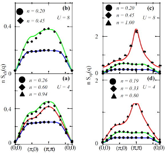
Figure 1: Wave vector ($\mathbf{q}$) dependence of the spin and charge structure factors for different sets of parameters. Solid lines are from TPSC and symbols are QMC data. Monte Carlo data for $n=1$ and $U=8t$ are for $6\times 6$ clusters and $T=0.5t$; all other data are for $8\times 8$ clusters and $T=0.2t$. Error bars are shown only when significant. From Ref. Tremblay:Vilk:1994 .

This figure allows one to watch the Pauli principle in action. At $U=4t,$ Fig.(1a) shows that the charge structure factor does not have a monotonic dependence on density. This is because, as we approach half-filling, the spin fluctuations are becoming so large that the charge fluctuations have to decrease so that the sum still satisfies the Pauli principle, as expressed by Eq.(10).

More comparisons may be found in Refs. Tremblay:LTP:2006 and Tremblay:Vilk:1994 ; Tremblay:Vilk:1997 ; Tremblay:Vilk:1996 ; Tremblay:Kyung:2003 . This kind of agreement is found even at couplings of the order of the bandwidth and when second-neighbor hopping $t^{\prime}$ is present Tremblay:Veilleux:1994 ; Tremblay:Veilleux:1995 .

Remark 3

Even though the entry in the renormalized classical regime is well described by TPSC Tremblay:Kyung:2003a , equation (13) for $U_{sp}$ fails deep in that regime because $\Sigma^{\left(1\right)}$ becomes too different from the true self-energy. At $n=1$, $t^{\prime}=0$, deep in the renormalized classical regime, $U_{sp}$ becomes arbitrarily small, which is clearly unphysical. However, by assuming that $\langle n_{\uparrow}n_{\downarrow}\rangle$ is temperature independent below $T_{X},$ a property that can be verified from QMC calculations, one obtains a qualitatively correct description of the renormalized-classical regime. One can even drop the ansatz and take $\langle n_{\uparrow}n_{\downarrow}\rangle$ from QMC on the right-hand side of the local moment sum-rule Eq.(16) to obtain $U_{sp}.$

0.2.3 Self-energy

Collective charge and spin excitations can be obtained accurately from Green’s functions that contain a simple self-energy, as we have just seen. Such modes are determined more by conservations laws than by details of the self-energy, especially at finite temperature where the lowest fermionic Matsubara frequency is not zero. The self-energy on the other hand is much more sensitive to collective modes since these are important at low frequency. The second step of TPSC is thus to find a better approximation for the self-energy. This is similar in spirit to what is done in the electron gas Tremblay:Mahan where plasmons are found with non-interacting particles and then used to compute an improved approximation for the self-energy. This two step process is also analogous to renormalization group calculations where renormalized interactions are evaluated to one-loop order and quasiparticle renormalization appears only to two-loop order Tremblay:Meyhnard:1973 ; Tremblay:Bourbonnais:1985 ; Tremblay:Zanchi:2001 .

The method to derive the result is justified using the formal derivation Tremblay:Allen:2003 that appears in Sect.0.2.5. If you are familiar with diagrams, you can understand physically the result by looking at Fig. 2 that shows the exact diagrammatic expressions for the three-point vertex (green triangle) and self-energy (blue circle) in terms of Green’s functions (solid black lines) and irreducible vertices (red boxes). The bare interaction $U$ is the dashed line. One should keep in mind that we are not using perturbation theory despite the fact that we draw diagrams. Even within an exact approach, the quantities defined in the figure have well defined meanings. The numbers on the figure refer to spin, space and imaginary time coordinates. When there is an over-bar, there is a sum over spin and spatial indices and an integral over imaginary time.

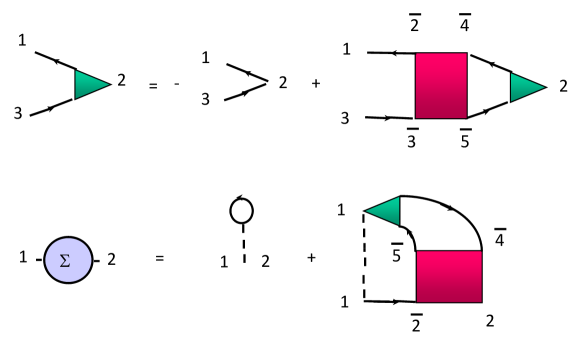
Figure 2: Exact expression for the three point vertex (green triangle) in the first line and for the self-energy in the second line. Irreducible vertices are the red boxes and Green’s functions solid black lines. The numbers refer to spin, space and imaginary time coordinates. Symbols with an over-bard are summed/integrated over. The self-energy is the blue circle and the bare interaction $U$ the dashed line.

In TPSC, the irreducible vertices in the first line of Fig. 2 are local, i.e. completely momentum and frequency independent. They are given by $U_{sp}$ and $U_{ch}.$ If we set point $3$ to be the same as point $1,$ then we can obtain directly the TPSC spin and charge susceptibilities from that first line. In the second line of the figure, the exact expression for the self-energy is displayed. The first term on the right-hand side is the Hartree-Fock contribution. In the second term, one recognizes the bare interaction $U$ at one vertex that excites a collective mode represented by the green triangle and the two Green’s functions. The other vertex is dressed, as expected. In the electron gas, the collective mode would be the plasmon. If we replace the irreducible vertex using $U_{sp}$ and $U_{ch}$ found for the collective modes, we find that here, both types of modes, spin and charge, contribute to the self-energy Tremblay:Vilk:1996 .

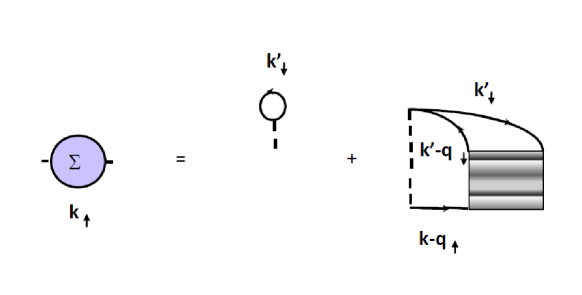
Figure 3: Exact self-energy in terms of the Hartree-Fock contribution and of the fully reducible vertex $\Gamma$ represented by a textured box.

There is, however, an ambiguity in obtaining the self-energy formula Tremblay:Moukouri:2000 . Within the assumption that only $U_{sp}$ and $U_{ch}$ enter as irreducible particle-hole vertices, the self-energy expression in the transverse spin fluctuation channel is different. What do we mean by that? Consider the exact formula for the self-energy represented symbolically by the diagram of Fig. 3. In this figure, the textured box is the fully reducible vertex $\Gamma\left(q,k-k^{\prime},k+k^{\prime}-q\right)$ that depends in general on three momentum-frequency indices. The longitudinal version of the self-energy corresponds to expanding the fully reducible vertex in terms of diagrams that are irreducible in the longitudinal (parallel spins) channel illustrated in Fig. 2. This takes good care of the singularity of $\Gamma$ when its first argument $q$ is near $\left(\pi,\pi\right).$ The transverse version Tremblay:Moukouri:2000 ; Tremblay:Allen:2003 does the same for the dependence on the second argument $k-k^{\prime}$, which corresponds to the other (antiparallel spins) particle-hole channel. But the fully reducible vertex obeys crossing symmetry. In other words, interchanging two fermions just leads to a minus sign. One then expects that averaging the two possibilities gives a better approximation for $\Gamma$ since it preserves crossing symmetry in the two particle-hole channels Tremblay:Moukouri:2000 . By considering both particle-hole channels only, we neglect the dependence of $\Gamma$ on $k+k^{\prime}-q$ because the particle-particle channel is not singular. The final formula that we obtain is Tremblay:Moukouri:2000

$$\Sigma_{\sigma}^{\left(2\right)}(k)=Un_{-\sigma}+\frac{U}{8}\frac{T}{N}\sum_{q}\left[3U_{sp}\chi_{sp}(q)+U_{ch}\chi_{ch}(q)\right]G_{\sigma}^{\left(1\right)}(k+q),$$ (26)

where $n_{-\sigma}$ is the average single-spin occupation. The superscript $\left(2\right)$ reminds us that we are at the second level of approximation. $G_{\sigma}^{\left(1\right)}$ is the same Green’s function as that used to compute the susceptibilities $\chi^{\left(1\right)}(q)$. Since the self-energy is constant at that first level of approximation, this means that $G_{\sigma}^{\left(1\right)}$ is the non-interacting Green’s function with the chemical potential that gives the correct filling. That chemical potential $\mu^{\left(1\right)}$ is slightly different from the one that we must use in $\left(G^{\left(2\right)}\right)^{-1}=i\omega_{n}+\mu^{\left(2\right)}-\varepsilon_{\mathbf{k}}-\Sigma^{\left(2\right)}$ to obtain the same density Tremblay:Kyung:2001 . Estimates of $\mu^{\left(1\right)}$ may be found in Ref. Tremblay:Allen:2003 ; Tremblay:Kyung:2001 ). Further justifications for the above formula are given below in Sect.0.2.4.

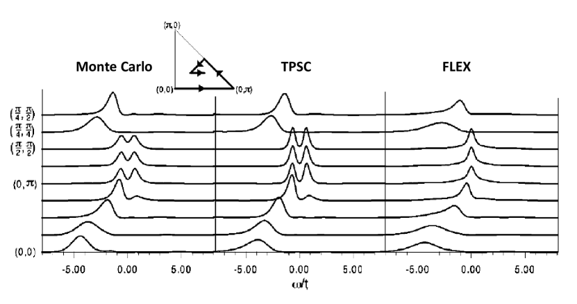
Figure 4: Single-particle spectral weight $A(\mathbf{k},\omega)$ for $U=4$, $\beta=5$, $n=1$, and all independent wave vectors $\mathbf{k}$ of an $8\times 8$ lattice. Results obtained from maximum entropy inversion of Quantum Monte Carlo data on the left panel, from TPSC in the middle panel and form the FLEX approximation on the right panel. (Relative error in all cases is about 0.3%). Figure from Ref.Tremblay:Moukouri:2000

But before we come up with more formalism, we check that the above formula is accurate by comparing in Fig. 4 the spectral weight (imaginary part of the Green’s function) obtained from Eq.(26) with that obtained from Quantum Monte Carlo calculations. The latter are exact within statistical accuracy and can be considered as benchmarks. The meaning of the curves are detailed in the caption. The comparison is for half-filling in a regime where the simulations can be done at very low temperature and where a non-trivial phenomenon, the pseudogap, appears. This all important phenomenon is discussed further below in subsection 0.2.6 and in the first case study, Sect. 0.3.1. In the third panel, we show the results of another popular Many-Body Approach, the FLuctuation Exchange Approximation (FLEX) Tremblay:Bickers:1989 . It misses Tremblay:Deisz:1996 the physics of the pseudogap in the single-particle spectral weight because it uses fully dressed Green’s functions and assumes that Migdal’s theorem applies, i.e. that the vertex does not need to be renormalized consequently Ref.Tremblay:Vilk:1997 ; Tremblay:Monthoux:2003 . The same problem exists in the corresponding version of the GW approximation. Tremblay:Hedin:1999

Remark 4

The dressing of one vertex in the second line of Fig. 2 means that we do not assume a Migdal theorem. Migdal’s theorem arises in the case of electron-phonon interactions Tremblay:Mahan:2000 . There, the small ratio $m/M,$ where $m$ is the electronic mass and $M$ the ionic mass, allows one to show that the vertex corrections are negligible. This is extremely useful in formulating the Eliashberg theory of superconductivity.

Remark 5

In Refs. Tremblay:Vilk:1997 ; Tremblay:Moukouri:2000 we used the notation $\Sigma^{\left(1\right)}$ instead of $\Sigma^{\left(2\right)}.$ The notation of the present paper is the same as that of Ref. Tremblay:Allen:2003

0.2.4 Internal accuracy checks

How can we make sure that TPSC is accurate? We have shown sample comparisons with benchmark Quantum Monte Carlo calculations, but we can check the accuracy in other ways. For example, we have already mentioned that the f-sum rule Eq.(15) is exactly satisfied at the first level of approximation (i.e. with $n_{\mathbf{k}}^{\left(1\right)}$ on the right-hand side). Suppose that on the right-hand side of that equation, one uses $n_{\mathbf{k}}$ obtained from $G^{\left(2\right)}$ instead of the Fermi function. One should find that the result does not change by more than a few percent. This is what happens when agreement with QMC is good.

When we are in the Fermi liquid regime, another way to verify the accuracy of the approach is to verify if the Fermi surface obtained from $G^{\left(2\right)}$ satisfies Luttinger’s theorem very closely.

Finally, there is a consistency relation between one- and two-particle quantities ($\Sigma$ and $\left\langle n_{\uparrow}n_{\downarrow}\right\rangle$). The relation

$$\frac{T}{N}\sum_{\mathbf{k}}\sum_{n}\Sigma(\mathbf{k},i\omega_{n})G(\mathbf{k},i\omega_{n})e^{-i\omega_{n}0^{-}}=\frac{1}{2}\mathrm{Tr}\left(\Sigma G\right)=U\left\langle n_{\uparrow}n_{\downarrow}\right\rangle$$ (27)

should be satisfied exactly for the Hubbard model. This result follows from the definition of self-energy and is derived in Eq.(40) below. In standard many-body books Tremblay:Mahan:2000 , it is encountered in the calculation of the free energy through a coupling-constant integration. In TPSC, it is not difficult to show that the following equation

$$\frac{1}{2}\mathrm{Tr}\left(\Sigma^{\left(2\right)}G^{\left(1\right)}\right)=U\left\langle n_{\uparrow}n_{\downarrow}\right\rangle$$ (28)

is satisfied exactly with the self-consistent $U\left\langle n_{\uparrow}n_{\downarrow}\right\rangle$ obtained with the susceptibilities. An internal accuracy check consists in verifying by how much $\frac{1}{2}\mathrm{Tr}\left(\Sigma^{\left(2\right)}G^{\left(2\right)}\right)$ differs from $\frac{1}{2}\mathrm{Tr}\left(\Sigma^{\left(2\right)}G^{\left(1\right)}\right).$ Again, in regimes where we have agreement with Quantum Monte Carlo calculations, the difference is only a few percent.

The above relation between $\Sigma$ and $\left\langle n_{\uparrow}n_{\downarrow}\right\rangle$ gives us another way to justify our expression for $\Sigma^{\left(2\right)}.$ Suppose one starts from Fig. 2 to obtain a self-energy expression that contains only the longitudinal spin fluctuations and the charge fluctuations, as was done in the first papers on TPSC Tremblay:Vilk:1994 . One finds that each of these separately contributes an amount $U\left\langle n_{\uparrow}n_{\downarrow}\right\rangle/2$ to the consistency relation Eq.(28). Similarly, if we work only in the transverse spin channel Tremblay:Moukouri:2000 ; Tremblay:Allen:2003 we find that each of the two transverse spin components also contributes $U\left\langle n_{\uparrow}n_{\downarrow}\right\rangle/2$ to $\frac{1}{2}\mathrm{Tr}\left(\Sigma^{\left(2\right)}G^{\left(1\right)}\right).$ Hence, averaging the two expressions also preserves rotational invariance. In addition, one verifies numerically that the exact sum rule (Ref. Tremblay:Vilk:1997 Appendix A)

$$-\int\frac{d\omega^{\prime}}{\pi}\Sigma_{\sigma}^{\prime\prime R}\left(\mathbf{k,}\omega^{\prime}\right)=U^{2}n_{-\sigma}\left(1-n_{-\sigma}\right)$$ (29)

determining the high-frequency behavior is satisfied to a higher degree of accuracy with the symmetrized self-energy expression Eq. (26).

Eq. (26) for $\Sigma^{\left(2\right)}$ is different from so-called Berk-Schrieffer type expressions Tremblay:Berk:1966 that do not satisfy the consistency condition between one- and two-particle properties, $\frac{1}{2}\mathrm{Tr}\left(\Sigma G\right)=$ $U\left\langle n_{\uparrow}n_{\downarrow}\right\rangle.$

Remark 6

Schemes, such as FLEX, that use on the right-hand side $G^{\left(2\right)}$ are thermodynamically consistent (Sect. 0.4.4) and might look better. However, as we just saw, in Fig. 4, FLEX misses some important physics. The reason Tremblay:Vilk:1997 is that the vertex entering the self-energy in FLEX is not at the same level of approximation as the Green’s functions. Indeed, since the latter contain self-energies that are strongly momentum and frequency dependent, the irreducible vertices that can be derived from these self-energies should also be frequency and momentum dependent, but they are not. In fact they are the bare vertices. It is as if the quasi-particles had a lifetime while at the same time interacting with each other with the bare interaction. Using dressed Green’s functions in the susceptibilities with momentum and frequency independent vertices leads to problems as well. For example, the conservation law $\chi_{sp,ch}\left(\mathbf{q=0}\text{{,}}i\omega_{n}\right)=0$ is violated in that case, as shown in Appendix A of Ref.Tremblay:Vilk:1997 . Further criticism of conserving approaches appears in Appendix E of Ref.Tremblay:Vilk:1997 and in Ref.Tremblay:Allen:2003 .

0.2.5 A more formal derivation

Details of a more formal derivation may be found in Ref. Tremblay:Allen:2001 . For completeness we repeat some of the derivation. The reader more interested in the physics may skip that section. The first two subsections present some general formalism that is then used in the following two subsections to derive TPSC.

Single-particle properties

Following functional methods of the Schwinger schoolTremblay:Baym:1962 ; Tremblay:BaymKadanoff:1962 ; Tremblay:MartinSchwinger:1959 , we begin with the generating function with source fields $\phi_{\sigma}$ and field destruction operators $\psi$ in the grand canonical ensemble

$$\ln Z\left[\phi\right]=\ln\mathrm{Tr}\left[e^{-\beta\left(\widehat{H}-\mu\widehat{N}\right)}\text{T}_{\tau}\left(e^{-\psi_{\overline{\sigma}}^{\dagger}\left(\overline{1}\right)\phi_{\overline{\sigma}}\left(\overline{1},\overline{2}\right)\psi_{\overline{\sigma}}\left(\overline{2}\right)}\right)\right]$$ (30)

We adopt the convention that $1$ stands for the position and imaginary time indices $\left(\mathbf{r}_{1},\tau_{1}\right).$ The over-bar means summation over every lattice site and integration over imaginary-time from $0$ to $\beta$, and $\overline{\sigma}$ summation over spins. T_τ is the time-ordering operator.

The propagator in the presence of the source field is obtained from functional differentiation

$$G_{\sigma}\left(1,2;\{\phi\}\right)=-\left\langle\psi_{\sigma}\left(1\right)\psi_{\sigma}^{\dagger}\left(2\right)\right\rangle_{\phi}=-\frac{\delta\ln Z\left[\phi\right]}{\delta\phi_{\sigma}\left(2,1\right)}.$$ (31)

From now on, the time-ordering operator in averages, $\left\langle{}\right\rangle$, is implicit. Physically relevant correlation functions are obtained for $\{\phi\}=0$ but it is extremely convenient to keep finite $\{\phi\}$ in intermediate steps of the calculation.

Using the equation of motion for the field $\psi$ and the definition of the self-energy, one obtains the Dyson equation in the presence of the source field Tremblay:KadanoffLivre:1962

$$\left(G_{0}^{-1}-\phi\right)G=1+\Sigma G\quad;\quad G^{-1}=G_{0}^{-1}-\phi-\Sigma$$ (32)

where, from the commutator of the interacting part of the Hubbard Hamiltonian $H,$ one obtains

$$\Sigma_{\sigma}\left(1,\overline{1};\{\phi\}\right)G_{\sigma}\left(\overline{1},2;\{\phi\}\right)=-U\left\langle\psi_{-\sigma}^{\dagger}\left(1^{+}\right)\psi_{-\sigma}\left(1\right)\psi_{\sigma}\left(1\right)\psi_{\sigma}^{\dagger}\left(2\right)\right\rangle_{\phi}.$$ (33)

The imaginary time in $1^{+}$ is infinitesimally larger than in $1$.

Response functions

Response (four-point) functions for spin and charge excitations can be obtained from functional derivatives $\left(\delta G/\delta\phi\right)$ of the source-dependent propagator. Following the standard approach and using matrix notation to abbreviate the summations and integrations we have,

$$GG^{-1}=1$$ (34)

$$\frac{\delta G}{\delta\phi}G^{-1}+G\frac{\delta G^{-1}}{\delta\phi}=0.$$ (35)

Using the Dyson equation (32) $G^{-1}=G_{0}^{-1}-\phi-\Sigma$ this may be rewritten

$$\frac{\delta G}{\delta\phi}=-G\frac{\delta G^{-1}}{\delta\phi}G=G_{\char 94\relax}G+G\frac{\delta\Sigma}{\delta\phi}G,$$ (36)

where the symbol _^ in $G_{\char 94\relax}G$ reminds us that the neighboring labels of the propagators have to be the same as those of the $\phi$ in the functional derivative. If perturbation theory converges, we may write the self-energy as a functional of the propagator. From the chain rule, one then obtains an integral equation for the response function in the particle-hole channel that is the analog of the Bethe-Salpeter equation in the particle-particle channel

$$\frac{\delta G}{\delta\phi}=G_{\char 94\relax}G+G\left[\frac{\delta\Sigma}{\delta G}\frac{\delta G}{\delta\phi}\right]G.$$ (37)

The labels of the propagators in the last term are attached to the self energy, as in Eq.(36) . Vertices appropriate for spin and charge responses are given, respectively, by

$$U_{sp}=\frac{\delta\Sigma_{\uparrow}}{\delta G_{\downarrow}}-\frac{\delta\Sigma_{\uparrow}}{\delta G_{\uparrow}}\quad;\quad U_{ch}=\frac{\delta\Sigma_{\uparrow}}{\delta G_{\downarrow}}+\frac{\delta\Sigma_{\uparrow}}{\delta G_{\uparrow}}.$$ (38)

TPSC First step: two-particle self-consistency for $G^{\left(1\right)},\Sigma^{\left(1\right)},$ $\Gamma_{sp}^{\left(1\right)}=U_{sp}$ and $\Gamma_{ch}^{\left(1\right)}=U_{ch}$

In conserving approximations, the self-energy is obtained from a functional derivative $\Sigma\left[G\right]=\delta\Phi\left[G\right]/\delta G$ of $\Phi$ the Luttinger-Ward functional, which is itself computed from a set of diagrams. To liberate ourselves from diagrams, we start instead from the exact expression for the self-energy, Eq.(33) and notice that when label $2$ equals $1^{+},$ the right-hand side of this equation is equal to double-occupancy $\left\langle n_{\uparrow}n_{\downarrow}\right\rangle$. Factoring as in Hartree-Fock amounts to assuming no correlations. Instead, we should insist that $\left\langle n_{\uparrow}n_{\downarrow}\right\rangle$ be obtained self-consistently. After all, in the Hubbard model, there are only two local four point functions: $\left\langle n_{\uparrow}n_{\downarrow}\right\rangle$ and $\left\langle n_{\uparrow}n_{\uparrow}\right\rangle=\left\langle n_{\downarrow}n_{\downarrow}\right\rangle.$ The latter is given exactly, through the Pauli principle, by $\left\langle n_{\uparrow}n_{\uparrow}\right\rangle=\left\langle n_{\downarrow}n_{\downarrow}\right\rangle=\left\langle n_{\uparrow}\right\rangle=\left\langle n_{\downarrow}\right\rangle=n/2,$ when the filling $n$ is known. In a way, $\left\langle n_{\uparrow}n_{\downarrow}\right\rangle$ in the self-energy equation (33), can be considered as an initial condition for the four point function when one of the points, $2$, separates from all the others which are at $1.$ When that label $2$ does not coincide with $1$, it becomes more reasonable to factor à la Hartree-Fock. These physical ideas are implemented by postulating

$$\Sigma_{\sigma}^{\left(1\right)}\left(1,\overline{1};\{\phi\}\right)G_{\sigma}^{\left(1\right)}\left(\overline{1},2;\{\phi\}\right)=A_{\{\phi\}}G_{-\sigma}^{\left(1\right)}\left(1,1^{+};\{\phi\}\right)G_{\sigma}^{\left(1\right)}\left(1,2;\{\phi\}\right)$$ (39a)

where $$A_{\{\phi\}}$$ depends on external field and is chosen such that the exact result

$$\Sigma_{\sigma}\left(1,\overline{1};\{\phi\}\right)G_{\sigma}\left(\overline{1},1^{+};\{\phi\}\right)=U\left\langle n_{\uparrow}\left(1\right)n_{\downarrow}\left(1\right)\right\rangle_{\phi}$$ (40)

is satisfied. It is easy to see that the solution is

$$A_{\{\phi\}}=U\frac{\left\langle n_{\uparrow}\left(1\right)n_{\downarrow}\left(1\right)\right\rangle_{\phi}}{\left\langle n_{\uparrow}\left(1\right)\right\rangle_{\phi}\left\langle n_{\downarrow}\left(1\right)\right\rangle_{\phi}}.$$ (41)

Substituting $A_{\{\phi\}}$ back into our ansatz Eq.(13) we obtain our first approximation for the self-energy by right-multiplying by $\left(G_{\sigma}^{\left(1\right)}\right)^{-1}:$

$$\Sigma_{\sigma}^{\left(1\right)}\left(1,2;\{\phi\}\right)=A_{\{\phi\}}G_{-\sigma}^{\left(1\right)}\left(1,1^{+};\{\phi\}\right)\delta\left(1-2\right).$$ (42)

We are now ready to obtain irreducible vertices using the prescription of the previous section, Eq.(38), namely through functional derivatives of $\Sigma$ with respect to $G.$ In the calculation of $U_{sp},$ the functional derivative of $\left\langle n_{\uparrow}n_{\downarrow}\right\rangle/\left(\left\langle n_{\uparrow}\right\rangle\left\langle n_{\downarrow}\right\rangle\right)$ drops out, so we are left with

$$U_{sp}=\left.\frac{\delta\Sigma_{\uparrow}^{\left(1\right)}}{\delta G_{\downarrow}^{\left(1\right)}}\right|_{\{\phi\}=0}-\left.\frac{\delta\Sigma_{\uparrow}^{\left(1\right)}}{\delta G_{\uparrow}^{\left(1\right)}}\right|_{\{\phi\}=0}=A_{\{\phi\}=0}=U\frac{\left\langle n_{\uparrow}n_{\downarrow}\right\rangle}{\left\langle n_{\uparrow}\right\rangle\left\langle n_{\downarrow}\right\rangle}.$$ (43)

The renormalization of this irreducible vertex may be physically understood as coming from Kanamori-Brueckner screening Tremblay:Vilk:1997 . This completes the derivation of the ansatz that was missing in our first derivation in section 0.2.1.

The functional-derivative procedure generates an expression for the charge vertex $U_{ch}$ which involves the functional derivative of $\left\langle n_{\uparrow}n_{\downarrow}\right\rangle/\left(\left\langle n_{\uparrow}\right\rangle\left\langle n_{\downarrow}\right\rangle\right)$ which contains six point functions that one does not really know how to evaluate. But, if we again assume that the vertex $U_{ch}$ is a constant, it is simply determined by the requirement that charge fluctuations also satisfy the fluctuation-dissipation theorem and the Pauli principle, as in Eq.(17).

Note that, in principle, $\Sigma^{\left(1\right)}$ also depends on double-occupancy, but since $\Sigma^{\left(1\right)}$ is a constant, it is absorbed in the definition of the chemical potential and we do not need to worry about it in this case. That is why the non-interacting irreducible susceptibility $\chi^{\left(1\right)}(q)=\chi_{0}(q)$ appears in the expressions for the susceptibility, even though it should be evaluated with $G^{\left(1\right)}$ that contains $\Sigma^{\left(1\right)}.$ A rough estimate of the renormalized chemical potential (or equivalently of $\Sigma^{\left(1\right)}$), is given in the appendix of Ref. Tremblay:Allen:2003 . One can check that spin and charge conservation are satisfied by our susceptibilities.

TPSC Second step: an improved self-energy $\Sigma^{\left(2\right)}$

Collective modes are emergent objects that are less influenced by details of the single-particle properties than the other way around. We thus wish now to obtain an improved approximation for the self-energy that takes advantage of the fact that we have found accurate approximations for the low-frequency spin and charge fluctuations. We begin from the general definition of the self-energy Eq.(33) obtained from Dyson’s equation. The right-hand side of that equation can be obtained either from a functional derivative with respect to an external field that is diagonal in spin, as in our generating function Eq.(30), or by a functional derivative of $\left\langle\psi_{-\sigma}\left(1\right)\psi_{\sigma}^{\dagger}\left(2\right)\right\rangle_{\phi_{t}}$ with respect to a transverse external field $\phi_{t}.$

Working first in the longitudinal channel, the right-hand side of the general definition of the self-energy Eq.(33) may be written as

$$\Sigma_{\sigma}\left(1,\overline{1}\right)G_{\sigma}\left(\overline{1},2\right)=-U\left[\left.\frac{\delta G_{\sigma}\left(1,2;\{\phi\}\right)}{\delta\phi_{-\sigma}\left(1^{+},1\right)}\right|_{\{\phi\}=0}-G_{-\sigma}\left(1,1^{+}\right)G_{\sigma}\left(1,2\right)\right].$$ (44)

The last term is the Hartree-Fock contribution. It gives the exact result for the self-energy in the limit $\omega\rightarrow\infty$.Tremblay:Vilk:1997 The $\delta G_{\sigma}/\delta\phi_{-\sigma}$ term is thus a contribution to lower frequencies and it comes from the spin and charge fluctuations. Right-multiplying the last equation by $G^{-1}$ and replacing the lower energy part $\delta G_{\sigma}/\delta\phi_{-\sigma}$ by its general expression in terms of irreducible vertices, Eq.(37) we find

$$\Sigma_{\sigma}^{\left(2\right)}\left(1,2\right) = UG_{-\sigma}^{\left(1\right)}\left(1,1^{+}\right)\delta\left(1-2\right)$$

$$-UG_{\sigma}^{\left(1\right)}\left(1,\overline{3}\right)\left[\left.\frac{\delta\Sigma_{\sigma}^{\left(1\right)}\left(\overline{3},2;\{\phi\}\right)}{\delta G_{\overline{\sigma}}^{\left(1\right)}\left(\overline{4},\overline{5};\{\phi\}\right)}\right|_{\{\phi\}=0}\left.\times\frac{\delta G_{\overline{\sigma}}^{\left(1\right)}\left(\overline{4},\overline{5};\{\phi\}\right)}{\delta\phi_{-\sigma}\left(1^{+},1\right)}\right|_{\{\phi\}=0}\right].$$

Every quantity appearing on the right-hand side of that equation has been taken from the TPSC results. This means in particular that the irreducible vertices $\delta\Sigma_{\sigma}^{\left(1\right)}/\delta G_{\sigma^{\prime}}^{\left(1\right)}$ are at the same level of approximation as the Green functions $G_{\sigma}^{\left(1\right)}$ and self-energies $\Sigma_{\sigma}^{\left(1\right)}.$ In approaches that assume that Migdal’s theorem applies to spin and charge fluctuations, one often sees renormalized Green functions $G^{\left(2\right)}$ appearing on the right-hand side along with unrenormalized vertices, $\delta\Sigma_{\sigma}/\delta G_{\sigma^{\prime}}\rightarrow U.$ In terms of $U_{sp}$ and $U_{ch}$ in Fourier space, the above formulaTremblay:Vilk:1996 reads,

$$\Sigma_{\sigma}^{\left(2\right)}(k)_{long}=Un_{-\sigma}+\frac{U}{4}\frac{T}{N}\sum_{q}\left[U_{sp}\chi_{sp}^{\left(1\right)}(q)+U_{ch}\chi_{ch}^{\left(1\right)}(q)\right]G_{\sigma}^{\left(1\right)}(k+q).$$ (46)

The approach to obtain a self-energy formula that takes into account both longitudinal and transverse fluctuations is detailed in Ref. Tremblay:Allen:2003 . Crossing symmetry, rotational symmetry and sum rules and comparisons with QMC dictate the final formula for the improved self-energy $\Sigma^{\left(2\right)}$ as we have explained in Sect.(0.2.3).

0.2.6 Pseudogap in the renormalized classical regime

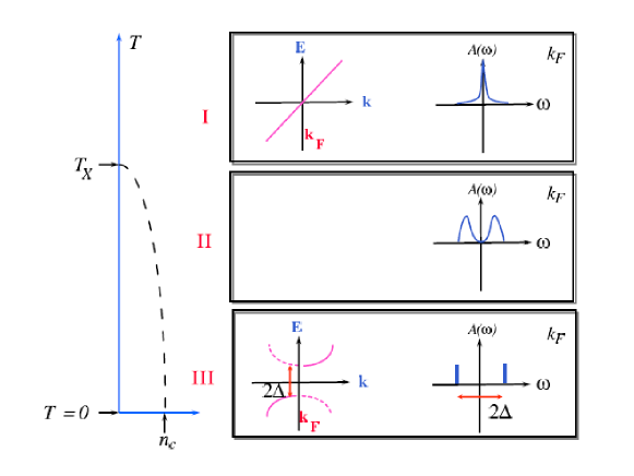
Figure 5: Cartoon explanation of the pseudogap due to precursors of long-range order. When the antiferromagnetic correlation length $\xi$ becomes larger than the thermal de Broglie wavelength, there appears precursors of the $T=0$ Bogoliubov quasi-particles for the long-range ordered antiferromagnet. This can occur only in the renormalized classical regime, below the dashed line on the left of the figure.

When we compared TPSC with Quantum Monte Carlo simulations and with FLEX in Fig. 4 above, perhaps you noticed that at the Fermi surface, the frequency dependent spectral weight has two peaks instead of one. In addition, at zero frequency, it has a minimum instead of a maximum. That is called a pseudogap. A cartoon explanation Tremblay:LTP:2006 of this pseudogap is given in Fig. 5. At high temperature we start from a Fermi liquid, as illustrated in panel I. Now, suppose the ground state has long-range antiferromagnetic order as in panel III, in other words at a filling between half-filling and $n_{c}$. In the mean-field approximation we have a gap and the Bogoliubov transformation from fermion creation-annihilation operators to quasi-particles has weight at both positive and negative energies. In two dimensions, because of the Mermin-Wagner theorem, as soon as we raise the temperature above zero, long-range order disappears, but the antiferromagnetic correlation length $\xi$ remains large so we obtain the pseudogap illustrated in panel II. As we will explain analytically below, the pseudogap survives as long as $\xi$ is much larger than the thermal de Broglie wave length $\xi_{th}\equiv v_{F}/(\pi T)$ in our usual units. At the crossover temperature $T_{X}$, the relative size of $\xi$ and $\xi_{th}$ changes and we recover the Fermi liquid.

We now proceed to sketch analytically where these results come from starting from finite $T$. Details and more complete formulae may be found in Refs. Tremblay:Vilk:1994 ; Tremblay:Vilk:1996 ; Tremblay:Vilk:1997 ; Tremblay:Vilk:1995 . We begin from the TPSC expression (26) for the self-energy. Normally one has to do the sum over bosonic Matsubara frequencies first, but the zero Matsubara frequency contribution has the correct asymptotic behavior in fermionic frequencies $i\omega_{n}$ so that, as in Sect.0.2.2, one can once more isolate on the right-hand side the contribution from the zero Matsubara frequency. In the renormalized classical regime then, we have

$$\Sigma(\mathbf{k}_{F},i\omega_{n})\propto T\int q^{d-1}dq\frac{1}{q^{2}+\xi^{-2}}\frac{1}{i\omega_{n}-\varepsilon_{\mathbf{k}_{F}+\mathbf{Q+q}}}$$ (47)

where $\mathbf{Q}$ is the wave vector of the instability. This integral can be done analytically in two dimensions Tremblay:Vilk:1997 ; Tremblay:VilkShadow:1997 . But it is more useful to analyze limiting cases Tremblay:Vilk:1996 . Expanding around the points known as hot spots where $\varepsilon_{\mathbf{k}_{F}+\mathbf{Q}}=0$, we find after analytical continuation that the imaginary part of the retarded self-energy at zero frequency takes the form

$$\Sigma^{\prime\prime R}(\mathbf{k}_{F},0) \propto-\pi T\int d^{d-1}q_{\perp}dq_{||}\frac{1}{q_{\perp}^{2}+q_{||}^{2}+\xi^{-2}}\delta(v_{F}^{\prime}q_{||})$$ (48)

$$\propto\frac{\pi T}{v_{F}^{\prime}}\xi^{3-d}.$$ (49)

In the last line, we just used dimensional analysis to do the integral.

The importance of dimension comes out clearly Tremblay:Vilk:1996 . In $d=4$, $\Sigma^{\prime\prime R}(\mathbf{k}_{F},0)$ vanishes as temperature decreases, $d=3$ is the marginal dimension and in $d=2$ we have that $\Sigma^{\prime\prime R}(\mathbf{k}_{F},0)\propto\xi/\xi_{th}$ that diverges at zero temperature. In a Fermi liquid the quantity $\Sigma^{\prime\prime R}(\mathbf{k}_{F},0)$ vanishes at zero temperature, hence in three or four dimensions one recovers the Fermi liquid (or close to one in $d=3$). But in two dimensions, a diverging $\Sigma^{\prime\prime R}(\mathbf{k}_{F},0)$ corresponds to a vanishingly small $A(\mathbf{k}_{F},\omega=0)$ as we can see from

$$A(\mathbf{k},\omega)=\frac{-2\Sigma^{\prime\prime R}(\mathbf{k}_{F},\omega)}{(\omega-\varepsilon_{\mathbf{k}}-\Sigma^{\prime R}(\mathbf{k}_{F},\omega))^{2}+\Sigma^{\prime\prime R}(\mathbf{k}_{F},\omega)^{2}}.$$ (50)

Fig. 31 of Ref.Tremblay:LTP:2006 illustrates graphically the relationship between the location of the pseudogap and large scattering rates at the Fermi surface. At stronger $U$ the scattering rate is large over a broader region, leading to a depletion of $A(\mathbf{k,}\omega)$ over a broader range of $\mathbf{k}$ values.

Remark 7

Note that the condition $\xi/\xi_{th}\gg 1$, necessary to obtain a large scattering rate, is in general harder to satisfy than the condition that corresponds to being in the renormalized classical regime. Indeed, $\xi/\xi_{th}\gg 1$ corresponds $T/v_{F}\gg\xi^{-1}$ while the condition $\omega_{sp}\ll T$ for the renormalized classical regime corresponds to $T\gg\xi^{-2},$ with appropriate scale factors, because $\omega_{sp}$ scales as $\xi^{-2}$ as we saw in Eq. (23) and below.

To understand the splitting into two peaks seen in Figs. 4 and 5 consider the singular renormalized contribution coming from the spin fluctuations in Eq. (47) at frequencies $\omega\gg v_{F}\xi^{-1}.$ Taking into account that contributions to the integral come mostly from a region $q\leq\xi^{-1}$, one finds

$$\Sigma^{\prime R}(\mathbf{k}_{F},\omega) =\left(T\int q^{d-1}dq\frac{1}{q^{2}+\xi^{-2}}\right)\frac{1}{ik_{n}-\varepsilon_{\mathbf{k}_{F}+\mathbf{Q}}}$$

$$\equiv\frac{\Delta^{2}}{\omega-\varepsilon_{\mathbf{k}_{F}+\mathbf{Q}}}$$ (51)

which, when substituted in the expression for the spectral weight (50) leads to large contributions when

$$\omega-\varepsilon_{\mathbf{k}}-\frac{\Delta^{2}}{\omega-\varepsilon_{\mathbf{k}_{F}+\mathbf{Q}}}=0$$ (52)

or, equivalently,

$$\omega=\frac{(\varepsilon_{\mathbf{k}}+\varepsilon_{\mathbf{k}_{F}+\mathbf{Q}})\pm\sqrt{(\varepsilon_{\mathbf{k}}-\varepsilon_{\mathbf{k}_{F}+\mathbf{Q}})^{2}+4\Delta^{2}}}{2},$$ (53)

which, at $\omega=0$, corresponds to the position of the hot spots. At finite frequencies, this turns into the dispersion relation for the antiferromagnet Tremblay:Zhang:1989 .

It is important to understand that analogous arguments hold for any fluctuation that becomes soft because of the Mermin-Wagner theorem,Tremblay:Vilk:1997 ; Tremblay:Davoudi:2008 including superconducting ones Tremblay:Vilk:1997 ; Tremblay:Allen:2001 ; Tremblay:Kyung:2001 . The wave vector $\mathbf{Q}$ would be different in each case.

To understand better when Fermi liquid theory is valid and when it is replaced by the pseudogap instead, it is useful to perform the calculations that lead to $\Sigma^{\prime\prime R}(\mathbf{k}_{F},0)\propto\xi/\xi_{th}$ in the real frequency formalism. The details may be found in Appendix D of Ref. Tremblay:Vilk:1997 .

0.3 Case studies

In this short pedagogical review it is impossible to cover all topics in depth. This section will nevertheless expand a bit on two important contributions of TPSC to problems of current interest, namely the pseudogap of cuprate superconductors and superconductivity induced by antiferromagnetic fluctuations.

0.3.1 Pseudogap in electron-doped cuprates

High-temperature superconductors are made of layers of CuO₂ planes. The rest of the structure is commonly considered as providing either electron or hole doping of these planes depending on chemistry. At half-filling, or zero-doping, the ground state is an antiferromagnet. As one dopes the planes, one reaches a doping, so-called optimal doping, where the superconducting transition temperature $T_{c}$ is maximum. Let us start from optimal hole or electron doping and decrease doping towards half-filling. That is the underdoped regime. In that regime, one observes a curious phenomenon, the pseudogap. What this means is that as temperature decreases, physical quantities behave as if the density of states near the Fermi level were decreasing. Finding an explanation for this phenomenon has been one of the major challenges of the field Tremblay:Timusk:1999 ; Tremblay:Norman:2005 .

To make progress, we need a microscopic model for high-temperature superconductors. Band structure calculations Tremblay:Andersen:1995 ; Tremblay:Andersen:2001 reveal that a single band crosses the Fermi level. Hence, it is a common assumption that these materials can be modeled by the one-band Hubbard model. Whether this is an oversimplification is still a subject of controversy Tremblay:peets:2009 ; Tremblay:Liebsch:2010 ; Tremblay:PhillipsComment:2010 ; Tremblay:Varma:2009 ; Tremblay:Macridin:2005 ; Tremblay:Hanke:2010 . Indeed, spectroscopic studies Tremblay:ChenX:1991 ; Tremblay:peets:2009 show that hole doping occurs on the oxygen atoms. The resulting hole behaves as a copper excitation because of Zhang-Rice Tremblay:Zhang:1988a singlet formation. In addition, the phase diagram Tremblay:Senechal:2005 ; Tremblay:maier_d:2005 ; Tremblay:Aichhorn:2006 ; Tremblay:Aichhorn:2007 ; Tremblay:Haule:2007 ; Tremblay:kancharla:2008 and many properties of the hole-doped cuprates can be described by the one-band Hubbard model. Typically, the band parameters that are used are: nearest-neighbor hopping $t=350\;$ to $400\;$meV and next-nearest-neighbor hopping $t^{\prime}=-0.15$ to $-0.3t$ depending on the compound Tremblay:Andersen:1995 ; Tremblay:Andersen:2001 . A third-nearest-neighbor hopping $t^{\prime\prime}=-0.5t^{\prime}$ is sometimes added to fit finer details of the band structure Tremblay:Andersen:2001 . The second-neighbor hopping breaks particle-hole symmetry at the band structure level.

In electron-doped cuprates, the doping occurs on the copper, hence there is little doubt that the single-band Hubbard model is even a better starting point in this case. Band parameters Tremblay:Massida:1989 are similar to those of hole-doped cuprates. It is sometimes claimed that there is a pseudogap only in the hole-doped cuprates. The origin of the pseudogap is indeed probably different in the hole-doped cuprates. But even though the standard signature of a pseudogap is absent in nuclear magnetic resonance Tremblay:Zheng:2003 (NMR) there is definitely a pseudogap in the electron-doped case as well Tremblay:Armitage:2010 , as can be seen in optical conductivity Tremblay:Onose:2001 and in Angle Resolved Photoemission Spectroscopy (ARPES) Tremblay:Armitage:2002 . As we show in the rest of this section, in electron-doped cuprates strong evidence for the origin of the pseudogap is provided by detailed comparisons of TPSC with ARPES as well as by verification with neutron scattering Tremblay:Motoyama:2007 that the TPSC condition for a pseudogap, namely $\xi>\xi_{th},$ is satisfied. The latter length makes sense from weak to intermediate coupling when quasi-particles exist above the pseudogap temperature. In strong coupling, i.e. for values of $U$ larger than that necessary for the Mott transition, there is evidence that there is another mechanism for the formation of a pseudogap. This is discussed at length in Refs. Tremblay:Senechal:2004 ; Tremblay:Hankevych:2006 . The recent discovery Tremblay:Sordi:2010 that at sufficiently large $U$ there is a first order transition in the paramagnetic state between two kinds of metals, one of which is highly anomalous, gives a sharper meaning to what is meant by strong-coupling pseudogap.

Let us come back to modeling of electron-doped cuprates. Evidence that these are less strongly coupled than their hole-doped counterparts comes from the fact that a) The value of the optical gap at half-filling, $\sim 1.5$ eV, is smaller than for hole doping, $\sim 2.0$ eV Tremblay:Tokura:1990 . b) In a simple Thomas-Fermi picture, the screened interaction scales like $\partial\mu/\partial n.$ Quantum cluster calculations Tremblay:Senechal:2004 show that $\partial\mu/\partial n$ is smaller on the electron-doped side, hence $U$ should be smaller. c) Mechanisms based on the exchange of antiferromagnetic fluctuations with $U/t$ at weak to intermediate coupling Tremblay:Bickers_dwave:1989 ; Tremblay:Kyung:2003 predict that the superconducting $T_{c}$ increases with $U/t$. Hence $T_{c}$ should decrease with increasing pressure in the simplest model where pressure increases hopping $t$ while leaving $U$ essentially unchanged. The opposite behavior, expected at strong coupling where $J=4t^{2}/U$ is relevant Tremblay:kancharla:2008 ; Tremblay:Kotliar:1988 , is observed in the hole-doped cuprates. d) Finally and most importantly, we have shown detailed agreement between TPSC calculations Tremblay:Kyung:2004 ; Tremblay:Hankevych:2006 ; Tremblay:LTP:2006 and measurements such as ARPES Tremblay:Armitage:2002 ; Tremblay:Matsui:2005 , optical conductivity Tremblay:Onose:2001 and neutron Tremblay:Motoyama:2007 scattering.

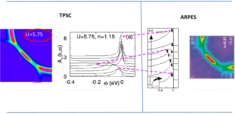
Figure 6: On the left, results of TPSC calculations Tremblay:Kyung:2004 ; Tremblay:LTP:2006 at optimal doping, $x=0.15,$ corresponding to filling $1.15,$ for $t=350$ meV, $t^{\prime}=-0.175t,$ $t\textquotedblright=0.05t,$ $U=5.75t,$ $T=1/20.$ The left-most panel is the magnitude of the spectral weight times a Fermi function, $A\left(\mathbf{k},\omega\right)f\left(\omega\right)$ at $\omega=0,$ so-called momentum-distribution curve (MDC). Red (dark black) indicates larger value and purple (light grey) smaller value. The next panel is $A\left(\mathbf{k},\omega\right)f\left(\omega\right)$ for a set of fixed $\mathbf{k}$ values along the Fermi surface. These are so-called energy-dispersion curves (EDC). The two panels to the right are the corresponding experimental results Tremblay:Armitage:2002 for Nd_2-xCe_xCuO${}_{4}.$ Dotted arrows show the correspondence between TPSC and experiment.

To illustrate the last point, consider Fig. 6 that compares TPSC calculations with experimental results for ARPES. Apart from a tail in the experimental results. the agreement is striking. . In particular, if there were no interaction, the Fermi surface would be a line (red) on the momentum distribution curve (MDC). Instead, it seems to disappear at symmetrical points displaced from $\left(\pi/2,\pi/2\right).$ These points, so-called hot spots, are linked by the wave vector $\left(\pi,\pi\right)$ to other points on the Fermi surface. This is where the antiferromagnetic gap would open first if there were long-range order. The pull back of the weight from $\omega=0$ at the hot spots is close to the experimental value: $100$ meV for the $15\%$ doping shown, and $300$ meV for $10\%$ doping (not shown). More detailed ARPES spectra and comparisons with experiment are shown in Ref. Tremblay:LTP:2006 . The value of the temperature $T^{\ast}$ at which the pseudogap appears Tremblay:Kyung:2004 is also close to that observed in optical spectroscopy Tremblay:Onose:2001 . In addition, the size of the pseudogap is about ten times $T^{\ast}$ in the calculation as well as in the experiments. For optical spectroscopy, vertex corrections (see Sect. 0.4.5) have to be added to be more quantitative. Experimentally, the value of $T^{\ast}$ is about twice the antiferromagnetic transition temperature up to $x=0.13$. That can be obtained Tremblay:Kyung:2004 by taking $t_{z}=0.03t$ for hopping in the third direction. Recall that in strictly two dimensions, there is no long-range order. Antiferromagnetism appears on a much larger range of dopings for electron-doped than for hole-doped cuprates.

These TPSC calculations have predicted the value of the pseudogap temperature at $x=0.13$ before it was observed experimentally Tremblay:Matsui:2005 by a group unaware of the theoretical prediction. In addition, the prediction that $\xi$ should scale like $\xi_{th}$ at the pseudogap temperature has been verified in neutron scattering experiments Tremblay:Motoyama:2007 in the range $x=0.04$ to $x=0.15$. At that doping, which corresponds to optimal doping, $T^{\ast}$ becomes of the order of $100$ K, more than four times lower than at $x=0.04.$ The antiferromagnetic correlation length $\xi$ beyond optimal doping begins to decrease and violate the scaling of $\xi$ with $\xi_{th}.$ In that doping range, $T^{\ast}$ and the superconducting transition temperature are close. Hence it is likely that there is interference between the two phenomena Tremblay:Sedeki:2009 , an effect that has not yet been taken into account in TPSC.

An important prediction that one should verify is that inelastic neutron scattering will find over-damped spin fluctuations in the pseudogap regime and that the characteristic spin fluctuation energy will be smaller than $k_{B}T$ whenever a pseudogap is present. Equality should occur above $T^{\ast}$.

Finally, note that the agreement found in Fig. 6 between ARPES and TPSC is for $U\sim 6t.$ At smaller values of $U$ the antiferromagnetic correlations are not strong enough to produce a pseudogap in that temperature range. For larger $U,$ the weight near $\left(\pi/2,\pi/2\right)$ disappears, in disagreement with experiments. The same value of $U$ is found for the same reasons in strong coupling calculations with Cluster Perturbation Theory (CPT) Tremblay:Senechal:2004 and with slave boson methods Tremblay:Yuan:2005 . Recent first principle calculations Tremblay:Weber:2010 find essentially the same value of $U.$ In that approach, the value of $U$ is fixed, whereas in TPSC it was necessary to increase $U$ by about $10\%$ moving towards half-filling to get the best agreement with experiment. In any case, it is quite satisfying that weak and strong coupling methods agree on the value of $U$ for electron-doped cuprates. This value of $U$ is very near the critical value for the Mott transition at half-filling Tremblay:park:2008 . Hence, antiferromagnetic fluctuations at finite doping can be very well described by Slater-like physics (nesting) in electron-doped cuprates.

For recent calculations including the effect of the third dimension on the pseudogap see Tremblay:Sedrakyan:2010 . Finally, note that the analog of the above mechanism for the pseudogap has also been seen in two-dimensional charge-density wave dichalcogenides Tremblay:Borisenko:2008 .

0.3.2 d-wave superconductivity

In the BCS theory of superconductivity, pairs of electrons form because of an effective attraction mediated by phonons. The pairs then condense in a coherent state. The suggestion that superconductivity could arise from purely repulsive forces goes back to Kohn and Luttinger who showed that for pairs of sufficiently high angular momentum, the screened Coulomb interaction in an electron gas could be attractive Tremblay:kohn:1965 . Just before the discovery of high-temperature superconductors, an extension of that idea was proposed Tremblay:Beal-Monod:1986 ; Tremblay:Scalapino:1986 ; Tremblay:Miyake:1986 . The suggestion was that antiferromagnetic fluctuations present in the Hubbard model could replace the phonons in BCS theory and lead to $d-$wave superconductivity. This is difficult to prove beyond any doubt since superconductivity in this case does not arise at the mean-field level. Mean-field on the Hubbard model gives antiferromagnetism near half-filling but not superconductivity. In the high-temperature superconductors, the situation is made even more difficult because of Mott Physics. Nevertheless, the question is well posed and, as we just saw, Mott physics might be less important in the electron-doped superconductors.

To investigate how the pairing susceptibility is influenced by antiferromagnetic fluctuations in TPSC we proceed as follows Tremblay:Kyung:2003 ; Tremblay:Hassan:2008 . The reader who did not go through the formal section 0.2.5 may skip the next paragraph without loss of continuity to read the physical results below. The few equations that appear below give details that are missing in the literature.

Some details of the derivation:

We work in Nambu space and add an off-diagonal source field $\theta$ and $\theta^{\ast}$ in the generating function Eq.(30). The transverse spin fluctuations are included by working with four by four matrices. The pair susceptibility in the normal state can be obtained from the second functional derivative of the generating function with respect to the off-diagonal source field, evaluated at zero source field. Tremblay:Kyung:2003 In more detail, one proceeds as in the formal derivation in Sect. 0.2.5. The expressions for the spin and charge susceptibilities are not modified. Once the two-particle quantities have been found as above, the second step of the approach Tremblay:Vilk:1997 ; Tremblay:Moukouri:2000 consists in improving the approximation for the single-particle self-energy by starting from the exact expression where the high-frequency Hartree-Fock behavior is explicitly subtracted

$$\mathbf{\Sigma}\left(1,2\right) = -U\left(\begin{tabular}[]{ll}$1$&$0$\\ $0$&$0$\end{tabular}\right)\frac{\delta\mathbf{G}\left(1,\overline{3}\right)}{\delta\phi_{\downarrow}\left(1^{+},1\right)}\mathbf{G}^{-1}\left(\overline{3},2\right)$$ (59)

$$+U\left(\begin{tabular}[]{ll}$0$&$0$\\ $0$&$1$\end{tabular}\right)\frac{\delta\mathbf{G}\left(1,\overline{3}\right)}{\delta\phi_{\uparrow}\left(1^{+},1\right)}\mathbf{G}^{-1}\left(\overline{3},2\right).$$

The bold face objects are matrices in Nambu space. To be able to express the right-hand side of the above equation in terms of irreducible vertices, susceptibilities and powers of $G,$ one differentiates $\mathbf{GG}^{-1}=\mathbf{I}$ to obtain $\left(\delta\mathbf{G/}\delta\phi\right)\mathbf{G}^{-1}=-\mathbf{G}\left(\delta\mathbf{G}^{-1}\mathbf{/}\delta\phi\right).$ With the help of Dyson’s equation on the right-hand side of the last equation as well as the chain rule, one finds an expression where one can replace every term by their value at the first step, namely $U_{sp}$ and $U_{ch}$ for the irreducible low-frequency vertices as well as $G_{\sigma}^{\left(1\right)}(k+q)$ and $\chi_{sp}(q),\chi_{ch}(q).$ For the diagonal piece of the self-energy at the second step, one then obtains Eq.(26) above or equivalently Eq.(3) of Ref.Tremblay:Moukouri:2000 ; Tremblay:Allen:2003 by considering both longitudinal and transverse channels and requiring crossing symmetry of the fully-reducible vertex in the two particle-hole channels as well as consistency with the sum-rule $\mathrm{Tr}\left(\Sigma^{\left(2\right)}G^{\left(1\right)}\right)=$ $2U\left\langle n_{\uparrow}n_{\downarrow}\right\rangle$ Tremblay:Vilk:1997 . The off-diagonal piece of the exact self-energy Eq.(59) on the other hand, reads

$$\Sigma_{12}^{\left(2\right)} = -UG_{11}^{\left(1\right)}\left(4,\overline{3}\right)\frac{\delta\Sigma_{12}^{\left(1\right)}\left(\overline{3},5\right)}{\delta\phi_{\downarrow}\left(4^{+},4\right)}$$

$$+UG_{12}^{\left(1\right)}\left(4,4^{+}\right)\delta\left(4-5\right)-UG_{12}^{\left(1\right)}\left(4,\overline{3}\right)\frac{\delta\Sigma_{22}^{\left(1\right)}\left(\overline{3},5\right)}{\delta\phi_{\downarrow}\left(4^{+},4\right)}.$$

The pairing susceptibility mediated by spin fluctuations may now be computed from the derivative with respect to the source field

$$\left.\frac{\delta G_{12}^{\left(2\right)}\left(1,3\right)}{\delta\theta\left(2,4\right)}\right|_{\theta=0} = G_{11}^{\left(2\right)}\left(1,2\right)G_{22}^{\left(2\right)}\left(4,3\right)$$

$$+G_{11}^{\left(2\right)}\left(1,\overline{4}\right)\left.\frac{\delta\Sigma_{12}^{\left(2\right)}\left(\overline{4},\overline{5}\right)}{\delta G_{12}^{\left(1\right)}\left(\overline{6},\overline{7}\right)}\right|_{\theta=0}\left.\frac{\delta G_{12}^{\left(1\right)}\left(\overline{6},\overline{7}\right)}{\delta\theta\left(2,4\right)}\right|_{\theta=0}G_{22}^{\left(2\right)}\left(\overline{5},3\right)$$

with the irreducible vertex $\delta\Sigma_{12}^{\left(2\right)}/\delta G_{12}^{\left(1\right)}$ obtained by functional differentiation of Eq.(Some details of the derivation:). Neglecting $\delta/\delta\phi_{\downarrow}\left(\delta\Sigma_{12}^{\left(1\right)}/\delta G_{12}^{\left(1\right)}\right),$ which represents the influence of spin fluctuations on the local piece of the irreducible vertex, and including the transverse component, we find for the d-wave pair susceptibility, $\chi_{d}$, the expression that appears in Eq.(1) of Ref. Tremblay:Kyung:2003 . The TPSC expression for the pair susceptibility $\chi_{d}$ contains the bubble part and the first term of what would be an infinite series if $\Sigma_{12}^{\left(2\right)}$ in the irreducible vertex could be differentiated with respect to $G_{12}^{\left(2\right)}$ instead of $G_{12}^{\left(1\right)}.$

Why should we trust the results for the d-wave susceptibility obtained for TPSC? Let us look again at benchmarks. Fig. 7(a) displays the d-wave susceptibility obtained from QMC calculations shown as symbols and from TPSC as lines. Because of the sign problem, it is not practical to do the QMC calculations at lower temperatures. Nevertheless, the temperatures are low enough that we see a non-trivial effect, the appearance of a maximum in susceptibility at finite doping and a substantial increase with decreasing temperatures. The agreement between QMC and TPSC is to within a few percent and improves for lower values of $U$. When the interaction strength reaches the intermediate coupling regime, $U=6$, deviations of the order of $20\%$ to $30\%$ may occur but the qualitative dependence on temperature and doping remains accurate. In TPSC the pseudogap is the key ingredient that leads to a decrease in $\chi_{d}$ in the underdoped regime. This is easy to understand since the pseudogap leaves fewer states for pairing at the Fermi level. Another way to say this is that the strong inelastic scattering that leads to the pseudogap is pair breaking. The inset shows that previous spin-fluctuation calculations (FLEX) in two dimensions Tremblay:Bickers_dwave:1989 ; Tremblay:Pao:1995 deviate both qualitatively and quantitatively from the QMC results. More specifically, in the FLEX approach $\chi_{d}$ does not show a pronounced maximum at finite doping. This is because, as we have shown in Fig.4, in FLEX there is no pseudogap in the single-particle spectral weight at the Fermi surface Tremblay:Deisz:1996 ; Tremblay:Moukouri:2000 .

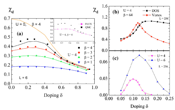
Figure 7: (Color online) From Ref.Tremblay:Kyung:2003 . (a) Comparisons between the $d_{x^{2}-y^{2}}$ susceptibility obtained from QMC simulations and from the approach described in the present work. QMC error bars are smaller than the symbols. Analytical results are joined by solid lines. Both calculations are for $U=4$, a $6\times 6$ lattice, and four different temperatures. The case $U=0$, $\beta=4$ is shown for reference. The size dependence of the results is small at these temperatures. The inset compares QMC and FLEX at $U=4$, $\beta=4$. (b) Contributions from the bubble (DOS) represented by squares and vertex represented by circles. (c) Estimate of $T_{c}$ using the Thouless criterion for $U=4$ and $U=6$, $t^{\prime}=t^{\prime\prime}=0$.

In two-dimensions, superconductivity is in the Kosterlitz-Thouless universality class. Vortex physics that is absent in TPSC is important to understand the precise value of the transition temperature. Nevertheless, a necessary condition for this transition to occur is that there is a higher temperature at which pairs form, a sort of mean-field $T_{c}.$ That $T_{c}$ can be obtained from the so-called Thouless criterion, i.e. from the temperature at which the d-wave susceptibility diverges. This divergence occurs because of growing vertex corrections. Since TPSC contains only the first term in what would be an infinite ladder sum, we take $T_{c}$ as the temperature at which the bubble (that we call DOS) and first term of the series (that we call vertex) become equal. This is illustrated in Fig. 7(b). At $\beta=1/64,$ the doping range between the intersection of the two curves is below $T_{c}.$ The resulting $T_{c}$ versus doping is shown in Fig. 7(c). In that calculation, $\left\langle n_{\uparrow}n_{\downarrow}\right\rangle$ is fixed at its value at $T^{\ast}.$

There is clearly an additional approximation in finding $T_{c}$ with TPSC that goes beyond what can be checked with QMC calculations. How can we be sure that this is correct? First there is consistency with other weak-coupling approaches. For example, Ref.Tremblay:Hankevych:2003 has shown consistency with cutoff renormalization group technique Tremblay:Honerkamp:2001 for competing ferromagnetic, antiferromagnetic and d-wave superconductivity. Second, there is consistency as well with Quantum Cluster Approaches that are best at strong-coupling. Indeed, an extensive study as a function of system size by the group of Jarrell Tremblay:maier_d:2005 has shown that for $10\%$ doping, $T_{c}$ is in the range $0.02,$ not far from $0.03$ that can be read from Fig. 7(c).

One of the major theoretical questions in the field of high-temperature superconductivity has been, “Is there d-wave superconductivity in the two-dimensional Hubbard model”? TPSC has contributed to answer this question. One of the most discouraging early results was that QMC simulations showed that the pairing susceptibility was smaller at finite $U$ than at $U=0.$ This is clearly seen in Fig. 7(a). TPSC allows us to understand why. At $\beta=4,$ the bubble largely dominates and the effect can only be pair breaking because of the inelastic scattering. The vertex, representing exchange of antiferromagnetic fluctuations analogous to the phonons in ordinary BCS theory, contributes $22\%$ at most at zero doping and much less at larger doping. Nevertheless, it clearly increases the pair susceptibility to bring it in closer agreement with QMC. TPSC allows us to do the calculation at temperatures much lower than QMC and to verify that indeed the vertex eventually grows large enough to lead to a transition. We understand also that in this parameter range the dome shape comes from the fact that antiferromagnetic fluctuations can both increase pairing through the vertex and be detrimental through the pseudogap produced by the large self-energy. Antiferromagnetic fluctuations can both help and hinder d-wave superconductivity.

Another question is whether the presence of a quantum critical point below the maximum of the superconducting dome plays a role in superconductivity. In the case we discussed above, long-range antiferromagnetic order appears at $T=0$ (not at finite $T$ because of Mermin-Wagner) up to doping $\delta=0.17$ for $U=4$ Tremblay:Kyung:2003 and $\delta=0.205$ for $U=6$ Tremblay:Bergeron:2011 . In this case, then, according to Fig. 7(c) the quantum critical point is far to the right of the maximum $T_{c}$ but superconductivity can exist to the right of that point, the more so when $U$ is larger.

How general are the above results? This and many more questions on the conditions for magnetically mediated superconductivity were studied with TPSC on the square lattice at half-filling for second-neighbor hopping $t^{\prime}$ different from zero Tremblay:Hassan:2008 . At $t^{\prime}=0$ at half-filling, there is a pseudogap on the whole Fermi surface because of perfect nesting, so $T_{c}$ vanishes. When $t^{\prime}$ is increased from zero, the pseudogap is not complete at half-filling and $T_{c}$ is different from zero. In addition, for $t^{\prime}$ larger than $0.71,$ the Fermi surface topology changes and the dominant magnetic fluctuations are near $\left(0,\pm\pi\right),\left(\pm\pi,0\right).$

Additional conclusions of the TPSC study of Ref. Tremblay:Hassan:2008 as a function of $t^{\prime}$ and $U$ at half-filling are as follows. First some qualitative conclusions that could be found from just the BCS gap equation with an interaction potential given by the static component of the spin susceptibility Tremblay:Scalapino:1995 : the symmetry of the d-wave order parameter is determined by the wave vector of the magnetic fluctuations. Those that are near $(\pi,\pi)$ lead to $d_{x^{2}-y^{2}}$-wave ($B_{1g}$) superconductivity while those that are near $(0,\pi)$ induce $d_{xy}$-wave ($B_{2g}$) superconductivity. The dominant wave vector for magnetic fluctuations is determined by the shape of the Fermi surface so $d_{x^{2}-y^{2}}$-wave superconductivity occurs for values of $t^{\prime}$ that are relatively small while $d_{xy}$-wave superconductivity occurs for $t^{\prime}>1$. Second, the maximum value that $T_{c}$ can take as a function of $t^{\prime}$ increases with interaction strength. TPSC cannot reach the strong-coupling regime where $T_{c}$ should decrease with $U$.

One also finds Tremblay:Hassan:2008 that, contrary to what is expected from BCS, the non-interacting single-particle density of states does not play a dominant role. At small $t^{\prime}$, $T_{c}$ is reduced by self-energy effects as discussed above and for intermediate values of $t^{\prime}$ the magnetic fluctuations are smaller and incommensurate so no singlet superconductivity appears. Hence at fixed $U$, there is an optimal value of $t^{\prime}$ (frustration) for superconductivity. For $d_{x^{2}-y^{2}}$ superconductivity in under-frustrated systems (small $t^{\prime}$) $T_{c}$ occurs below the temperature $T_{X}$ where the crossover to the renormalized classical regime occurs. In other words, in under-frustrated systems at $T_{c}$ the antiferromagnetic correlation length is much larger than the thermal de Broglie wave length and the renormalized classical spin fluctuations dominate. The opposite relationship between these lengths occurs for over-frustrated systems ($t^{\prime}$ larger than optimal) where $T_{c}$ is larger than $T_{X}$ and hence occurs in a regime where renormalized classical fluctuations do not dominate. The two temperatures, $T_{c}$ and $T_{X}$, are comparable for optimally frustrated systems. In all cases, at $T_{c}$ the antiferromagnetic correlation length is larger than the lattice spacing.

Superconductivity induced by antiferromagnetic fluctuations in weak to intermediate coupling has also been studied by Moriya and Ueda Tremblay:Moriya:2003 with the self-consistent renormalized approach that also satisfies the Mermin-Wagner theorem. However, in that approach there are adjustable parameters and no guarantee that the Pauli principle is satisfied so one cannot be certain this is an accurate solution to the Hubbard model.

That there is d-wave superconductivity in the two-dimensional Hubbard model has by now been seen by a number of different approaches: variational Tremblay:Giamarchi:1991 ; Tremblay:Paramekanti:2004 , various Quantum Cluster approaches Tremblay:Senechal:2005 ; Tremblay:maier_d:2005 ; Tremblay:Aichhorn:2006 ; Tremblay:Aichhorn:2007 ; Tremblay:Haule:2007 ; Tremblay:kancharla:2008 functional renormalization group Tremblay:Honerkamp:2003 , and even at asymptotically small $U$ by renormalization group Tremblay:Raghu:2010 . The retardation that can be observed even tells us that spin fluctuations remain important for d-wave superconductivity even at strong coupling Tremblay:Maier:2008 ; Tremblay:Kyung:2009 ; Tremblay:Hanke:2010 . The most serious objection to the existence of d-wave superconductivity comes from a variational and a gaussian Quantum Monte Carlo approach in Ref.Tremblay:Aimi:2007 . It could be that d-wave superconductivity in the two-dimensional Hubbard model is not the absolute minimum but only a local one. If this were the case, one could conclude that a small interaction term is missing in the Hubbard model to make the d-wave state the ground state. All other studies show that the physical properties of that state are very close the those of actual materials.

0.4 More insights on the repulsive model

The following two sections of this Chapter give a short summary of other results obtained with TPSC. The purpose is to show what has already been done, leading to the last section that contains a few open problems that could possibly be treated with TPSC. These two sections have some of the flavor of a review article, not that of a pedagogical introduction. In addition, an important aspect of a real review article is missing: there are very few references to the rest of the literature on any given topic. For anyone interested in pursuing some of these problems, the citation index is highly recommended.

0.4.1 Critical behavior and phase transitions

The self-consistent renormalized approach of Moriya-Lonzarich-Taillefer Tremblay:Moriya:1985 ; Tremblay:Lonzarich:1985 was one of the first ones to treat the Hubbard model in two dimensions in a way that satisfies the Mermin-Wagner theorem. Other approaches exist for the half-filling case: Schwinger bosons Tremblay:Arovas:1988 or constrained spin-waves Tremblay:Takahashi:1987 . The drawback of Moriya’s approach is that it contains several fitting parameters. Kanamori screening, discussed in Sect.0.2.2, is put by hand, as is the value of the mode coupling constant. In addition, nothing guarantees the Pauli principle. In other words, Moriya’s approach has much of the same physics as TPSC but it cannot be considered an accurate solution to the Hubbard model. There is also no prescription to compute the self-energy in a way that is consistent with double occupancy.

More generally, the question that arises with TPSC is whether it predicts the correct universality class. It was shown in Ref. Tremblay:Dare:1996 that its results are in the universality class of the spherical model, namely $O\left(N=\infty\right)$ instead of $O\left(N=3\right)$ as it should be for the Hubbard model with spin-rotation invariance. This result is not surprising since the self-consistency condition on double occupancy found from the local moment sum rule Eq. (16) is very similar to the self-consistency condition for the spherical model. With the standard convention for critical exponents, one finds $\gamma/\nu=2,z=2,$ and for dimension $d$ such that the condition $2<d<4$ is satisfied, we find $\nu=1/\left(d-2\right).$ This gives in $d=3,\nu=1,\gamma=2,\beta=1/2,\eta=0$ and $\delta=5.$ This should be compared with numerical results Tremblay:Pfeuty:1977 for the 3D Heisenberg $\left(n=3\right)$ model, $\nu=0.7$ and $\gamma=1.4.$ Clearly, too close to the critical point, or too deep in the renormalized classical regime in $d=2,$ TPSC looses its accuracy. Results in three dimensions can be found in Refs.Tremblay:Albinet:2000 ; Tremblay:Arita:2000 .

Crossover to 3d Tremblay:Dare:1996

The crossover from two- to three-dimensional critical behavior of nearly antiferromagnetic itinerant electrons was also studied in a regime where the interplane single-particle motion of electrons is quantum mechanically incoherent because of thermal fluctuations. The universal renormalized classical crossover function from $d=2$ to $d=3$ for the susceptibility has been explicitly computed, as well as a number of other properties such as the dependence of the Néel temperature on the ratio between hopping in the plane $t_{\shortparallel}$ and the hopping perpendicular to it, $t_{\perp},$

$$\frac{1}{T_{N}}\sim\frac{T_{N}^{2}}{U_{mf,c}^{2}}\left|\ln\left(\frac{t_{\shortparallel}}{t_{\perp}}\right)\right|$$ (62)

with $U_{mf,c}\equiv 2/\chi\left(\mathbf{Q}_{d=2},0\right)$ at the $d=2$ pseudogap temperature Tremblay:Dare:1996 .

Quantum critical behavior

At $T=0,$ half-filling, the ground state has long-range antiferromagnetic order. As one dopes, the order becomes incommensurate and eventually disappears at a critical point that is called “quantum critical” because it occurs at $T=0.$ Such quantum critical points are common in heavy-fermion systems for example. One of the surprising things about this critical point is that it affects the physics at surprisingly large $T.$

The quantum critical behavior of TPSC in $d=2$ is in the $z=2$ universality class, like the self-consistent renormalized theory of Moriya Tremblay:Moriya:1990 . Like that theory, it includes some of the logarithmic corrections found in the renormalization group approach Tremblay:RoschRMP:2007 . In addition, TPSC can be quantitative and answer the question, “How far in $T$ does the influence of that point extend?” It was found Tremblay:Roy:2008 ; Tremblay:RoyPhD:2007 by explicit numerical calculations away from the renormalized classical regime of the $d=2$ Hubbard model that logarithmic corrections are not really apparent in the range $0.01t<T<t$ and that the maximum static spin susceptibility in the $(T,n)$-plane obeys quantum critical scaling. However, near the commensurate-incommensurate crossover, one finds obvious non-universal $T$ and filling $n$ dependence. Everywhere else, the $(T,n)$-dependence of the non-universal scale factors is relatively weak. Strong deviations from scaling occur at $T$ of order $t$, the degeneracy temperature. That high temperature limit should be contrasted with $J/2$ found in the strong coupling case Tremblay:Kopp:2005 . In generic cases the upper limit $T\sim t$ is well-above room temperature. In experiment however, the non-universality due to the commensurate-incommensurate crossover may make the identification of quantum critical scaling difficult. In addition, note that properties other than the maximum spin susceptibility may deviate from quantum critical scaling at a lower temperature Tremblay:Bergeron:2011 .

0.4.2 Longer range interactions

Suppose one adds nearest-neighbor repulsion $V$ to the Hubbard model. The TPSC ansatz Eq. (39a) can be generalized Tremblay:Davoudi:2006 ; Tremblay:Davoudi:2007 . Then one needs to compute the effect of functional derivatives of the pair-correlation functions that appear, as in Sect. 0.2.5, in the calculation of spin and charge irreducible vertices. Since the Pauli principle and local spin and charge sum rules do not suffice, the functional derivatives are evaluated assuming particle-hole symmetry, which remains approximately true when the physics is dominated by states close to the Fermi surface. The resulting theory, called ETPSC, for Extended TPSC, satisfies conservation laws and the Mermin-Wagner theorem and is in agreement with benchmark quantum Monte Carlo results. This approach allows to reliably determine the crossover temperatures toward renormalized-classical regimes, and hence, the dominant instability as a function of $U$ and $V$. Contrary to RPA, even the spin fluctuations are modified by the presence of $V.$ Phase diagrams have been calculated. In the presence of $V$, charge order will generally compete with spin order Tremblay:Davoudi:2006 ; Tremblay:Davoudi:2007 .

0.4.3 Frustration

The ETPSC formalism outlined in the previous section is particularly important to treat interesting problems such as that of the sodium cobaltates. These compounds are often modeled in an over-simplified way by the two-dimensional Hubbard model on the triangular lattice. To account for charge fluctuations, one must also include nearest-neighbor repulsion $V.$ Even with this complication this is an oversimplified model.

The density- and interaction-dependent crossover diagram for spin- and charge-density wave instabilities of the normal state at arbitrary wave vector has been computed Tremblay:Davoudi:2008 . When $U$ dominates over $V$ and electron filling is large, instabilities are mostly in the spin sector and are controlled by Fermi surface properties. Increasing $V$ eventually leads to charge instabilities where it is mostly the wave vector dependence of the vertex that determines the wave vector of the instability rather than Fermi surface properties. At small filling, nontrivial instabilities appear only beyond the weak coupling limit. Charge-density wave instabilities are favored over a wide range of dopings by large $V$ at wave vectors corresponding to $\sqrt{3}$ $\times\sqrt{3}$ superlattice in real space. Commensurate fillings do not play a special role for this instability. Increasing $U$ leads to competition with ferromagnetism. At negative values of $U$ or $V$, neglecting superconducting fluctuations, one finds that charge instabilities are favored. In general, the crossover diagram presents a rich variety of instabilities. Thermal charge-density wave fluctuations in the renormalized-classical regime can open a pseudogap in the single-particle spectral weight, just as spin or superconducting fluctuations Tremblay:Davoudi:2008 .

0.4.4 Thermodynamics, conserving aspects

Conserving approaches are very popular. FLEX Tremblay:Bickers:1989 ; Tremblay:Bickers_dwave:1989 is an example. These approaches are attractive because they guarantee that if one evaluates the same physical quantity directly from the Green function or from a derivative of the free energy, the answer will be identical. All that is needed for a “conserving” approximation is that the self-energy be generated from a Luttinger Ward functional Tremblay:LuttingerWard:1960 that enters the expression for the free energy. In addition, conservation laws will be satisfied in transport if irreducible vertices are obtained from functional derivatives of the self-energy. This gives a so-called $\Phi$ derivable theory. Since in perturbation theory there is an infinite number of possible such Luttinger-Ward functionals, depending on which closed two-particle irreducible diagrams constructed from $G$ and the bare interaction one wishes to keep, the constraint of being conserving is not a very restrictive one. Conserving approximations do not satisfy the Pauli principle in general and they sometimes give negative values of double occupancy Tremblay:Arita:2000 . Various other limitations of conserving approaches are discussed in Appendix E of Ref. Tremblay:Vilk:1997 .

TPSC is not obtained from a functional derivative of a Luttinger Ward functional. Is this a drawback? We have seen that it satisfies conservation laws for spin and charge at the first step. The question is whether one can find a unique free energy that is consistent with the one-particle Green function and collective modes that TPSC focuses on. This question was addressed in the MSc Tremblay:RoyMSc:2002 and PhD thesis Tremblay:RoyPhD:2007 of Sébastien Roy. The results are summarized below. We conclude with an example of thermodynamic calculation in the context of cold atoms.

Thermodynamic consistency

We should really distinguish conservation laws and thermodynamic consistency. These two notions are sometimes confused, as outlined in the previous paragraph. We call an approach thermodynamically consistent when all possible ways of computing the same thermodynamic quantity give the same result.

Obtaining the self-energy from a functional derivative of the Luttinger-Ward functional leads to thermodynamic consistency. In TPSC there is a change in perspective. Instead of looking for an approximation for the free energy and then deducing everything else consistently, we find a single particle Green’s function $G^{\left(2\right)},$ or equivalently $\Sigma^{\left(2\right)},$ as well as double occupancy

$$\frac{1}{2}\mathrm{Tr}\left(\Sigma^{\left(2\right)}G^{\left(2\right)}\right)=U\left\langle n_{\downarrow}n_{\uparrow}\right\rangle^{\left(2\right)}.$$ (63)

and deduce everything else: The free energy from integration and the irreducible vertices for transport quantities from functional derivatives of $\Sigma^{\left(2\right)}$(Sect. 0.4.5).

There are three ways to extract the free energy from integration: (a) coupling constant integration of double occupancy (b) integration of $\mu(n)$ and (c) integration of the specific heat calculated from the total energy. With the free energy, all thermodynamic quantities can be obtained. If we make sure that the three ways to compute the free energy give the same result, then there is thermodynamic consistency.

With the above expression for double occupancy, Eq.(63), the three different ways of obtaining the thermodynamic quantities are all based on the same object $G^{\left(2\right)}.$ If $G^{\left(2\right)}\;$ were the exact solution, they would have to be consistent. However $G^{\left(2\right)}$ is approximate. Since $G^{\left(2\right)}$ satisfies all the requirements for a physical Green function, it is likely to be the exact solution of some Hamiltonian $H$ that is close to, but slightly different from, the Hubbard model. For example, $H$ could have longer range interactions. In deriving the formulas for the free energy, we assume that we are working with the Hubbard model. Hence, there is no guarantee that all three methods of obtaining $F$ will give the same result. One can check this numerically in principle. A simpler test, admittedly less stringent, is to compare $n\left(T,\mu,U\right)$ obtained from derivatives of the three different $F.$’s For the nearest-neighbor hopping model with $\beta=10,$ $U=4$ for example, the results are identical in the percent range, except deep in the renormalized classical regime close to half-filling where TPSC anyway fails Tremblay:RoyMSc:2002 ; Tremblay:RoyPhD:2007 .

The specific heat was calculated for the nearest-neighbor hopping Hubbard model at half-filling as a function of temperature. TPSC reproduces the peak observed at small temperature in QMC Tremblay:Paiva:2001 . It is associated with the entrance in the renormalized classical regime. Physically, the low temperature peak is a remnant of the specific heat jump that would occur at finite temperature in mean-field theory.

Cold atoms, entropy

In the context of cold atoms on optical lattices, adiabatic cooling can be used to reach interesting low $T$ regimes such as the pseudogap or ordered phases by manipulating the scattering length or the strength of the laser-induced lattice potential. TPSC has been used Tremblay:Dare:2007 , and compared with QMC calculations, to provide isentropic curves for the two- and three-dimensional Hubbard models at half-filling. Since double occupancy$\ D$ is extremely accurate in TPSC, the entropy $S$ was computed by integrating the Maxwell relation

$$\left(\frac{\partial S}{\partial U}\right)_{T,n}=-\left(\frac{\partial D}{\partial T}\right)_{U,n}$$ (64)

with $S\left(T,U=0\right)$ the known constant of integration.

The main findings are that adiabatically turning on the interaction in $d=2$ to cool the system is not very effective. In three dimensions, adiabatic cooling to the antiferromagnetic phase can be achieved in such a manner, although the cooling efficiency is not as high as initially suggested by dynamical mean-field theory Tremblay:WernerHassan:2005 . Adiabatic cooling by turning off the repulsion beginning at strong coupling is possible in certain cases.

0.4.5 Vertex corrections and conservation laws

Using the functional derivative formalism of Baym and Kadanoff, Tremblay:BaymKadanoff:1962 it is possible to find an expression within TPSC for the optical conductivity that satisfies conservation laws and hence the f-sum rule. In other words, one can include vertex corrections. Note that the f-sum rule this times involves the momentum distribution $n_{\mathbf{k}}^{\left(2\right)}$ obtained from the best self-energy.

The two types of vertex corrections that are found Tremblay:Bergeron:2011 are the antiferromagnetic analogs of the Aslamasov-Larkin and Maki-Thompson contributions of superconducting fluctuations to the conductivity but, contrary to the latter, they include non-perturbative effects. The calculations are impossible unless a number of advanced numerical algorithms are used. Take the case with nearest-neighbor hopping only.Tremblay:Bergeron:2011 In the pseudogap regime induced by two-dimensional antiferromagnetic fluctuations, the effect of vertex corrections is dramatic. Without vertex corrections the resistivity increases as we enter the pseudogap regime. Instead, vertex corrections lead to a drop in resistivity, as observed in a number of high temperature superconductors. At high temperature, the resistivity naturally saturates at the Ioffe-Regel limit. At the quantum critical point and beyond, the resistivity displays both linear and quadratic temperature dependence. The disappearance of superconductivity in the over-doped regime is correlated with the disappearance of the linear term in the $T$ dependence of the resistivity Tremblay:Cooper:2009 ; Tremblay:Auban:2009 . The relation to the physics of hot spots and results for other band structures ($t^{\prime}\neq 0$) should appear soon.

0.5 Attractive Hubbard model

Working in Nambu space and following a formal procedure analogous to that explained in Sect. 0.2.5, one can derive TPSC for the attractive Hubbard model Tremblay:Allen:2001 ; Tremblay:Allen:2003 ; Tremblay:AllenPhD:2000 . The irreducible vertex $U_{pp}$ in the particle-particle singlet channel is given by

$$U_{pp}\left\langle n_{\downarrow}\right\rangle\left\langle\left(1-n_{\uparrow}\right)\right\rangle=U\left\langle n_{\downarrow}\left(1-n_{\uparrow}\right)\right\rangle$$ (65)

and is determined self-consistently at the two-particle level by the local pair sum-rule

$$\left\langle n_{\downarrow}n_{\uparrow}\right\rangle=\langle\Delta^{\dagger}\Delta\rangle=\frac{T}{N}\sum_{q}\chi_{p}^{\left(1\right)}(q)\exp(-i\omega_{n}0^{-})$$ (66)

with

$$\chi_{p}^{\left(1\right)}(q)=\frac{\chi_{0}^{\left(1\right)}(q)}{1+U_{pp}\chi_{0}^{\left(1\right)}(q)}$$ (67)

and the irreducible particle-particle susceptibility

$$\chi_{0}^{\left(1\right)}(q)=\frac{T}{N}\sum_{k}G_{\sigma}^{\left(1\right)}(q-k)G_{-\sigma}^{\left(1\right)}(k)\;.$$ (68)

Again the Pauli principle and a number of crucial sum rules are satisfied. So is the Mermin-Wagner theorem.

In the second step of the approximation, an improved expression for the self-energy is obtained by using the results of the first step in an exact expression for the self-energy, to obtain,

$$\Sigma_{\sigma}^{\left(2\right)}(k)=Un_{-\sigma}-U\frac{T}{N}\sum_{q}U_{pp}\chi_{p}^{\left(1\right)}(q)G_{-\sigma}^{\left(1\right)}(q-k),$$ (69)

where $q=\left(i\omega_{n},\mathbf{q}\right).$ This is a cooperon-like formula. The required vertex corrections are included as required by the absence of a Migdal theorem. Comparisons with other approaches can be found in Ref.Tremblay:Verga:2005 .

Pseudogap from superconductivity in attractive Hubbard model

Using the TPSC for the attractive Hubbard model, quantitative agreement with Monte Carlo calculations is obtained for both single-particle and two-particle quantities Tremblay:Kyung:2001 . As discussed for the repulsive case in Sect.(0.2.6) one obtains a pseudogap in both the density of states and the single-particle spectral weight below some characteristic temperature $T^{\ast}$. It was even checked in QMC calculations that the ratio of the thermal de Broglie wavelength to the pairing correlation length must be larger than unity to observe the pseudogap Tremblay:Allen:1999 . The pseudogap, also found in Ref.Tremblay:Rohe:2001 for example, reflects precursors of Bogoliubov quasiparticles that are not local pairs, contrary to what is often discussed in the context of the crossover from BCS to Bose Einstein condensation Tremblay:Randeria:1992 .

With increasing temperature the spectral weight fills in the pseudogap instead of closing it Tremblay:Kyung:2001 . This type of behavior is obtained in high-temperature superconductors. The pseudogap appears earlier in the density of states than in the spectral function. A characteristic behavior observed at strong coupling appears already in TPSC at weak to intermediate coupling, namely, small temperature changes around $T^{\ast}$ can modify the spectral weight over frequency scales much larger than temperature Tremblay:Kyung:2001 .

Our earlier discussion about Kosterlitz-Thouless physics in Sect.(0.3.2) is valid in this case as well. In the attractive Hubbard model, the superconducting transition temperature has a dome shape because at half-filling the symmetry is SO$\left(3\right)$ so the $T_{c}$ there vanishes while it is given by the finite Kosterlitz-Thouless $T_{c}$ Tremblay:Moreo:1992 elsewhere. The pseudogap temperature on the other hand decreases monotonically from half-filling where it is largest. This exemplifies the fact that symmetry and dimension are important to understand pseudogap physics at weak to intermediate coupling Tremblay:Allen:1999 .

0.6 Open problems

At weak to intermediate coupling, TPSC gives the best agreement with benchmark Quantum Monte Carlo methods. Its strength, compared with all other methods, resides in a non-perturbative treatment of the Hubbard model that satisfies the Pauli principle and the Mermin-Wagner theorem, in addition to a number of other exact constraints. Also, one works in the infinite size limit so the effect of collective fluctuations is not limited to a small lattice like in dynamical mean-field theory Tremblay:Georges:1996 and its generalizations Tremblay:Maier:2005 ; Tremblay:KotliarRMP:2006 .

The main weakness of TPSC is the difficulty to extend the method beyond the one-band Hubbard model. One needs to find enough sum rules to determine the irreducible vertices. This can be seen as a challenge and an opportunity for creativity.

For example, to include nearest-neighbor Coulomb repulsion, one needs a way to evaluate functional derivatives of pair correlation functions to obtain irreducible vertices. It has been possible achieve this Tremblay:Davoudi:2007 , as discussed in Sect.(0.4.2), but every new problem is different. As another example, take the case of more than one band. Then the irreducible vertices become a matrix in band index and one does not have enough obvious sum rules to evaluate all the matrix elements Tremblay:Dare:unpublished .

In the presence of, say, antiferromagnetism the number of irreducible vertices also multiplies and one faces the same type of challenge. To treat long-range ordered states with TPSC, it might be easier to start with simpler broken symmetries such as ferromagnetism or the Pomeranchuk instability Tremblay:HalbothPom:2000 . The interest of treating long range order is clear. For example, the renormalized classical regime of antiferromagnetic fluctuations is presently inaccessible if $T$ is much smaller than $T^{\ast}.$ Starting from the ordered state may offer and alternative Tremblay:borejsza:2004 .

The question of the interplay of disorder and interactions is a difficult but topical one. Far from the Anderson disorder-induced metal-insulator transition, the impurity averaging technique Tremblay:AGD may prove a useful way to introduce disorder in TPSC. One may then answer the question of what happens to the $\xi>\xi_{th}$ criterion for pseudogap when the mean-free path becomes shorter than the thermal de Broglie wave length.

Climbing the ladder of difficult problems, the case of strong coupling Tremblay:Georges:1996 ; Tremblay:Maier:2005 ; Tremblay:KotliarRMP:2006 is a real challenge. At strong coupling the self-energy is singular at small frequencies. In fact it diverges as $1/\omega$ at half-filling. This is inconsistent with the starting point of TPSC where the self-energy is constant. Perhaps there is a way to start from the self-energy in the atomic limit inspired by methods that allow for multiple poles to zeroth order Tremblay:Mancini:2004 , or some other way Tremblay:Saso:2000 , but it is an unsolved problem for now.

Some problems, by contrast, appear straightforward but they can be very tedious. For example, in the presence of incommensurate magnetic fluctuations where singlet d-wave pairing does not occur, can triplet pairing take over? One can proceed along the lines of the derivation for d-wave superconductivity Tremblay:Hassan:2008 but with matrix source fields to generate triplet pairing in the Nambu formalism. The irreducible pairing vertex would again be obtained from functional derivatives of a matrix $\Sigma^{\left(2\right)}.$

Paring in the attractive Hubbard model is much more straightforward, as we have seen. It appears at the first step, without the need to generate irreducible vertices from $\Sigma^{\left(2\right)}.$ Nevertheless, to study the triplet channel in the attractive Hubbard model, one needs to introduce near-neighbor attraction $V$. That leads to the problems mentioned above in the repulsive case. As a curiosity, one could also investigate whether functional derivatives of $\Sigma^{\left(2\right)}$ in the attractive Hubbard model can mediate formation of order in some particle-hole channel. This might be a first step towards developing a method to take into account the different channels on the same footing in TPSC, Tremblay:Fresard:2000 as is done in renormalization group approaches Tremblay:HonerkampFRG:2001 ; Tremblay:HonerkampSalmhofer:2001 . It has been found recently within the renormalization group that in quasi one-dimensional systems there is a strong interference between antiferromagnetism and unconventional superconductivity Tremblay:Sedeki:2009 .

Proceeding along the lines of Ref. Tremblay:Bergeron:2011 for the conductivity, it is also clearly possible to compute other transport quantities, such as the thermopower, but it is a serious computational challenge.

There are roadblocks, but there are also opportunities for original solutions and breakthroughs.