Geometry of Injection Regions
of Power Networks
Abstract
We investigate the constraints on power flow in networks and its implications to the optimal power flow problem. The constraints are described by the injection region of a network; this is the set of all vectors of power injections, one at each bus, that can be achieved while satisfying the network and operation constraints. If there are no operation constraints, we show the injection region of a network is the set of all injections satisfying the conservation of energy. If the network has a tree topology, e.g., a distribution network, we show that under voltage magnitude, line loss constraints, line flow constraints and certain bus real and reactive power constraints, the injection region and its convex hull have the same Pareto-front. The Pareto-front is of interest since these are the the optimal solutions to the minimization of increasing functions over the injection region. For non-tree networks, we obtain a weaker result by characterize the convex hull of the voltage constraint injection region for lossless cycles and certain combinations of cycles and trees.
I Introduction
Optimal power flow is a classic problem in power engineering. It is usually given as a static subproblem of the security constraint unit commitment problem, in the sense that all the network dynamics such as transients and generator behaviors are abstracted away [1]. The objective of the optimal power flow problem is to minimize the cost of power generation in a electrical network while satisfying a set of operation constraints. The cost functions are generally taken to be convex and increasing. This problem has received considerable attention since the late 1960’s [2], and many different algorithms have been developed for it. For a comprehensive review the reader can consult [3] and the references within. Despite all the efforts, the optimal power flow problem still remains difficult [4].
The optimal power flow problem is difficult for two reasons. Firstly, the optimization problem is nonlinear since the power injected at each of the buses in the network depends quadratically on the voltages at the buses. Secondly, there is typically a large number of different types of constraints. For example, each bus might have voltage magnitude together with real and reactive power limits, and each transmission line might have thermal constraints and line flow constraints. Due to these two reasons, the optimal power flow problem is a non-convex optimization problem with many constraints, and is therefore challenging to solve. The traditional approach is to tackle the problem using various heuristics and approximations. One widely used method is to use the so called DC flow approximation where all the lines are assumed to be lossless, all voltage magnitude are assumed to be fixed, and all angle differences are assumed to be small [5]. To contrast with the DC flow approximation, the original optimal power flow problem is sometimes called the AC problem. As pointed out in [5], the DC approximation performs badly if it is not used in conjunction with a full AC solution (so called hot start DC) or if the resistance to inductance (R/X) ratio of the lines are high. To solve the full AC problem, many global optimization heuristics like genetic algorithms are used, and their effectiveness is generally gauged by simulations. But these algorithms do not offer any guarantees about performance and do not offer intuition into the structure of the optimization problem.
A new approach to the traditional optimization methods was taken by the authors in [6]. They made the surprising empirical observation that in many of the IEEE benchmark networks the optimal power flow problem has the same optimal value as its convex dual. The main theoretical result is that for a purely resistive network and quadratic cost functions with positive coefficients, this convex relaxation is tight. In addition, the result still holds if the purely resistive network is perturbed by adding a small reactive part. From this and their observations about the IEEE benchmarks, [6] conjectured that the convex relaxation of the optimal power flow problem is always tight for general networks. Unfortunately this conjecture is not true since there exist many counter examples [7, 8]. A natural question arises: if the relaxation is not tight in general, is it tight for some specific class of networks? The results [6] showed that for ’almost’ purely resistive networks the problem is convex, but these networks are somewhat unrealistic since practical power networks are mostly reactive instead of resistive. An impetus for this paper is to look for some more realistic classes of network for which the optimal power flow problem is convexified.
One increasingly important class of networks is the distribution network. The electricity network is made up of two layers: the transmission network and the distribution network. The transmission network consists of high voltage lines that connect big generators to cities and towns. The distribution network usually consists of a feeder connected to the transmission network, and low voltage lines that connect to the end consumers. In addition to the line voltages, the two types of networks have different topologies. The transmission network is sparse, but irregular, whereas the distribution network is configured to be a tree at any one time of operation. Traditionally, the optimal power flow problem is only solved in the transmission network, since the demands in the distribution network are fixed and there is very little generation, so there is nothing to optimize. But this is expected to change significantly under the new ’smart grid’ operating paradigm, where demand response and distributed renewable energy will play a predominant role. In the widely discussed demand response mechanism, the demands in the distribution network are decision variables (subjected to some constraints) [9, 10]. Also, due to increased renewable penetration at the demand level (e.g. rooftop solar) and increased distributed generation, solving the optimal power flow in the distribution network is a legitimate problem and could contribute to various pricing and control operations. For example, we show that the voltage control problem [11] can be formulated into such a framework. Since the resistance to inductance () ratio is much higher in the distribution network compared to the transmission network, DC approximations would perform poorly. Therefore, the full AC optimal power flow on the distribution network needs to be solved and we show the tree topology of the distribution network simplifies the problem significantly and allows the full AC problem to be efficiently solved in many situations.
To find out if the optimal power flow problem is convex for a network, we focus on the feasible injection region of a power network since it allows one to think about power flow in a more abstract way and is quite useful in understanding the structure of the problem. The feasible injection region is simply the feasibility region of the optimal power flow problem, i.e. the set of all vectors of feasible real power injections (both generations and withdraws) at the various buses that satisfy the given network and operation constraints (including reactive power constraints). For notational convenience, we drop the word feasible and refer to the region as the injection region. Since the optimization problem is solved over the injection region, it is useful to understand the geometry of the region. We model the reactive powers in the network as constraints at the buses. Therefore the injection region is in terms of the real powers, while possibly satisfying some bus reactive power constraints.
Unfortunately, the injection region is not convex in general [12]. Even though the region is not convex, it still has some desirable properties for optimization. A subset of the injection region of particular interest is the Pareto-front.111A point in a set is called Pareto-optimal if any coordinate cannot be decreased further without increasing at least one other coordinate; the Pareto front of a set is simply the set of all Pareto-optimal points. When minimizing an increasing function over a set, the optimal solutions are on the Pareto-front. Therefore, even though the injection region is not convex, if its Pareto-front is the same as that of its convex hull, the optimization problem is still easy.
The use of injection region is also useful since it decouples the optimization problem from the physics of power flow, thus allowing us to have a higher level view that is often beneficial for other problems in optimization, control and pricing in power systems. For example, [13] showed there is revenue adequacy in the financial transmission rights markets if the injection region has a convex Pareto-front. A similar observation is made by [14] in the context of economic dispatch. This result then can be used if the DC flow assumption is made or if the network is such that the AC injection region where the above condition is true. This is similarly the case for many of the recently proposed demand response algorithms.
As a starting point, we look at the injection region of a network with no constraints. In this case, we show the injection region is simply the upper half space that satisfies the law of conservation of energy. Therefore, the difficult and interesting part is to quantify how the injection region changes once the operation constraints are added.
There are typically four types of operation constraints in a power network: voltage magnitude, thermal loss in transmission lines, line flow limits in a transmission line and bus real and reactive power limits. If the network is a tree, we show that under voltage magnitude, line loss constraints, line flow constraints and certain bus power constraints, the injection region and its convex hull have the same Pareto-front. Precisely, the condition on the bus power constraints is: each bus is allowed to have real and reactive power upper bounds, but two connected buses cannot both simultaneously have real power lower bounds and there are no reactive power lower bounds. Through simulations with practical distribution networks, we show that these requirements are not stringent in actual operations. Independent works [15, 16] considered the OPF problem for a tree network, although the authors there used the notion of load over-satisfaction and did not consider thermal loss constraints.
The paper is organized as follows. In Section II we establish the notations, Section III contains the result about the network with no operation constraints, Section IV contains theoretical and simulations results concerning trees, and Section V concludes the paper. The Appendices contain the results about non-tree networks and some of the proofs.
The appendix address network with cycles. In some distribution systems, the network consists of a ring (cycle) feeder and tree networks hanging off the ring, therefore it is useful to understand the injection region of cycles. Ideally, one would like to state an analogous result as in the tree network case. However, we could not yet prove such a strong result. Instead, we characterize the convex hull of the voltage magnitude constrained injection region if the network is a cycle with lossless links and certain combinations of these networks with trees.
II Model and Notations
We consider the AC power flow model so in general all variables are complex. Following the convention in power engineering, scalars representing voltage, current and power are denoted with capital letters. We use to denote vectors, and to denote matrices. denote the element-wise product between and . Given two real vectors and of the same dimension, the notation denotes component-wise inequality and denotes component-wise inequality with strict inequality in at least one component. We denote Hermitian transpose by and complex conjugation by . We write to mean positive semidefinite. Given a set , denote the convex hull of , i.e. the smallest convex set containing .
Consider an electric network with buses. Throughout we assume the network is connected. We write if bus is connected to , and if they are not connected. Let denote the complex impedance of the transmission line between bus and bus , and . We have , and we assume that the lines are inductive (as in the Pi model) so . Note that and . Let () denote the shunt impedance (admittance) of bus to ground. These shunt impedances can come from the capacitance to ground in the Pi model of the transmission line, the capacitor banks installed for reactive power injection, or modeling constant impedance loads. The bus admittance matrix is denoted by and defined as
| (1) |
is symmetric. If the entries of are real, we say the network is purely resistive and if the entries are imaginary, we say the network is lossless. Lines in the transmission network are mainly inductive so it is sometimes assumed that the network is lossless. Let be the vector of bus voltages and be the vector of currents, where is the total current flowing out of bus to the rest of the network. By Ohm’s law and Kirchoff’s Current Law, . The complex power injected at bus is where is the real power and is the reactive power. A positive means bus is generating real power and a negative means bus is consuming real power; similarly for . Let be the vector of real powers and be the vector of reactive powers.
The real power vector where is the vector of diagonal elements of a matrix . Similarly, the reactive power vector . The resistive loss on a transmission line between buses and bus is given by . The powers flowing from bus to bus is denoted and , and defined as . Note .
II-A OPF Problem
In power networks, we are often interested in solving the following OPF problem
| minimize | (2a) | |||
| subject to | (2b) | |||
| (2c) | ||||
| (2d) | ||||
| (2e) | ||||
| (2f) | ||||
| (2g) | ||||
where is the cost function (not necessarily quadratic) defined on the real powers; (2b), (2c), (2d), (2e) and (2f) are the constraints corresponding to bus voltage, line thermal loss, line power flow and bus real and reactive power respectively; and (2g) is the physical law coupling voltage to power. The thermal loss constraints in (2c) are calculated from current rating of transmission lines and are usually the dominant constraints in distribution networks [17]. Typically the data sheet of a line would have a maximum current rating of the line, and this gives , the maximum loss that can be tolerated across a line. In practice, is usually an increasing function of the power injections. For example, if , then we are minimizing the loss in the network; or if is quadratic with positive coefficients, then we are minimizing the cost of generation.
In the rest of the paper we look at the feasible injection region, , defined as
| (3) |
Therefore is the feasibility region of (2). Note the reactive powers are represented as a constraint of the injection region. This is because in most practical settings, the objective function of the optimization problem is in terms of real powers only. For example, the cost curve for an generator only includes the real power output; also, the consumers are only charged based on the amount of real power they consume (watt-hours). Since the objective function is in terms of real powers only, the injection region is the set of all real injections.
III Network with No Operation Constraints
To warm up, let us first consider a network with no operation constraints. Since there are no constraints, the injection region is defined as
| (4) |
The reactive powers are ignored since we model reactive power as constraints in (2). In this case, the injection region has a simple characterization.
Theorem 1.
If the network is lossy222Every line has non-zero resistance, then is given by
| (5) |
Therefore is the union of the open upper half space of and the origin . Note this region is connected and convex. If the network is lossless, then is given by
| (6) |
Therefore is a hyperplane through the origin.
This result is intuitive pleasing since it says if there are no constraints in the network then the injection region is only limited by the law of conservation of energy. Conservation of energy gives the bound , and if the network is not lossless then except when all voltages are equal. In this case, all injections are so . Theorem 1 states this is the only constraint on the injection region. The authors in [18, 13] conjectured that the unconstrained injection region is convex, and (5) shows this is indeed the case. To proof this theorem, it is necessary to show that for every vector , there exists a voltage that achieves . The details are given in the Appendix.
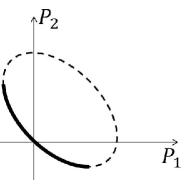
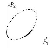
In practice, some of the constraints in (2) would be binding. For example, the voltages magnitudes at each bus are bounded. Figure 2(a) shows the injection region of a two bus network with fixed voltage magnitudes. The region is an ellipse (without the interior). Even in this simple case, we see that the injection region is no longer convex. The next section is devoted to the study of the effect of constraints on the injection regions of tree networks and their implications to optimization problems.
IV Tree Networks
IV-A Pareto-Front of Injection Region
In this section we consider the full problem in (2) for a tree network. The relevant geometric objects are the Pareto-optimal points of defined as:
Definition 1.
Let . A point is said to be a Pareto-optimal point if there does not exist another point such that . Denote the set of Pareto-optimal points of as and is sometimes called the Pareto-front of .333Here we actually consider only the non-degenerative Pareto-optimal points. For a precise definition see [19]. In almost all applications, the set of degenerative Pareto-optimal points are of measure 0 and does not correspond to the minima of strictly increasing functions.
The Pareto-optimal points of are of interest because only they can be the optimal solutions to (2) when is increasing. Under many circumstances, the Pareto-front of the injection region is the same as the Pareto-front of . Therefore, (2) is a convex optimization problem if is convex and increasing, since we may replace the non-convex region by a convex region and obtain the same solutions. Before stating the general result about the Pareto-front of in Theorem 2, it is instructive to use a two bus example to see what are the Pareto-optimal points and the effect of various kinds of constraints on them.
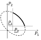
Consider the two bus example in Figure 1 where is the line admittance.
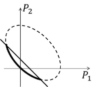
First consider the case where there are only voltage constraints. Suppose that per unit. Then is an ellipse as shown in Figure 2(a). The bold curve represents the Pareto-front. Note is the filled ellipse. We can see that the Pareto-fronts of the empty and the filled ellipses are the same. Therefore, if we replace the non-convex empty ellipse by the convex filled ellipse in an optimization problem with increasing objective function, we would obtain the same solution. Next, we consider both voltage constraints and the loss constraint for some . This is presented by intersecting the ellipse by a half plane as in Figure 2(b), and the bold curve is the resulting Pareto-front, and we see that it is again the same as the Pareto-front of .
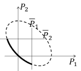
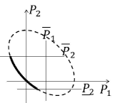
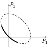
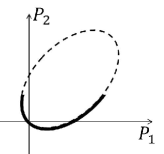
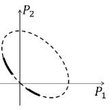
Next, consider both voltage and bus power constraints. In this case, there are several possibilities, as represented in Figures 3(a), 3(b) and 3(c). In Figure 3(a), both bus have power upper bounds, and the Pareto-front of is the same as the Pareto-front of . In Figure 3(b), has upper bound, has both upper and lower bounds, and the Pareto-front of is the same as the Pareto-front of . In Figure 3(c), both buses have lower bounds, and we see that the Pareto-front of is not the same as the Pareto-front of .
Next let us consider the effect of reactive power bounds. Figure 4(b) shows the feasible reactive power that can be achieved under the voltage constraint and the bold segment that satisfies the reactive power constraint . The bold segments in Figure 4(a) shows the corresponding injection region. As we can see, the Pareto-front of is the same as the Pareto-front of . Next, Figure 4(d) shows the bold segments that satisfies the constraint . As we can see, the Pareto-front of the Pareto-front of is not the same as the Pareto-front of Therefore, in general we cannot extend the result to include reactive power lower bounds.
The intuition gained from the two bus example carries over for general trees, and the general statement is given in Theorem 2.
Theorem 2.
Consider a tree network with buses. Let the injection region defined as in (3). Suppose two conditions are satisfied:
-
1.
If , then either or .
-
2.
for all .
The Pareto-front of is the same as the Pareto-front of .
The condition on the bus power lower bounds means that if two buses are connected, then not both can have a tight bus real power lower bound. Also, the theorem requires that all the reactive lower bounds to be not tight. This can be seen as a generalization of the well known load over-satisfaction concept [20]. In load over-satisfaction, all the lower bounds on real and reactive power are removed. But Theorem 2 states it is not necessary to remove all the lower bounds.
Proof:
To prove the theorem, first we define an optimization problem in term of the injection region. In this optimization problem, we want to write every quantity as a quadratic form of the complex voltages.
The resistive loss on the transmission line between buses and can be written as where is a matrix with the th entry and the th entry being , and the th entry and the th entry being and all other entries being . The power flow from bus to bus can be written as , where is a matrix with th entry , the th entry , the th entry and all the other entries . Let where is the diagonal matrix with at the entry and everywhere else. Similarly let . Then the powers injected at bus is given by and .
Consider the following optimization problem
| (7) | ||||
| subject to | ||||
The ’s can be interpreted as the costs of the power generation and (7) is an optimal power flow problem with a linear cost function. To expose the potential non-convexity, we can equivalently write it as
| (8) | ||||
| subject to | ||||
where and the non-convexity enters as the rank 1 constraint on . Relaxing this rank constraint and eliminating and , we get
| (9) | ||||
| subject to | ||||
where and . Note is Hermitian.
Geometrically, the relaxation from (3) to (9) enlarges the feasible injection region to a convex region given by
| (10) | ||||
We want to show that the two regions have the same Pareto-front. That is, . Since is convex, its Pareto-front is easily explored. Note in general and the inclusion can be strict. However, if and have the same Pareto-front, then so does .
The proof of the theorem follows from the following claim.
Claim 3.
Suppose for all . Then the optimal solution to (9) is unique and has rank if for every connected pair of buses in the network, one of them do not have tight bus power lower bound, and all reactive power lower bounds are not tight.
This claim is a stronger statement then saying , it also states that the optimal solution to the relaxed solution is unique. Assuming for now the claim is true. Then since is convex, we can explore its Pareto-front by linear functions with positive costs [21]. More precisely, a point is a Pareto-optimal if and only if it is an optimal solution to (9) for some positive costs. From the claim, all the optimal solutions are achieved by a of rank , therefore they can be achieved by using a voltage vector . Therefore if is a Pareto-optimal, then . Since , is also a Pareto-optimal point of . So . To show the other direction, suppose there exists a point but not in . Then there is a point such that . But , contradicting the fact is a Pareto-optimal point of . Therefore and thus . It remains to prove claim 3.
We are to show that the optimal solution to (9), , is rank 1. We do this through duality theory. The dual of (9) is
| maximize | ||||
| subject to | ||||
| (11) |
where and are the Lagrange multiplier associated with the voltage upper and lower bounds and and , are the Lagrange multiplier associated with the thermal constraints, and are the Lagrange multipliers associated with the flow constraints, and and are the Lagrange multiplier associated with the power upper and lower bounds and . Since we assume that the reactive power lower bounds constraints are not tight, is the Lagrange multiplier associated with the reactive power upper bounds. Note (11) is also the dual of (7) so the gap between and is called the duality gap.
Let . Let denote the optimal solution of (9) and the optimal solution of (11), by the complimentary slackness condition [21],
| (12) |
Since both and are positive semidefinite, (12) implies that . Therefore is in the null space of and . So to show it suffices to show . This is done by considering the topology of the network and thus the structure of .
Given a matrix and a graph with nodes, we say that fits if for , if and only if is not an edge in . The values on the diagonal of are unconstrained. The next lemma from [22] relates the topology of a graph and the rank of matrix that fits it.
Lemma 4 (Theorem 3.4 in [22]).
Let be a graph that is a connected tree of nodes. Suppose is a complex positive semidefinite matrix that fits . Then .
We want to apply this lemma to the matrix . Since is diagonal, only matters and its th entry, is given by
Therefore if if bus is not connected to bus . For to fit the network, needs to be nonzero if is connected to .
If , for to be zero we need
| (13) | ||||
| (14) | ||||
Multiplying (13) by and (14) by and adding we get
We are to show that . If this not the case, then suppose and . But since it is a Lagrange multiplier and , this contradicts (14). Similarly, since (lines are inductive), we cannot have and . Therefore we get the simultaneous equations in (15) and (16).
| (15) | ||||
| (16) | ||||
Note , and are always nonnegative since they are the Lagrange multipliers associated with upper bounds. Suppose the bus power lower bound is not tight for bus , then . Adding (15) with (16) gives , this is not possible since . On the other hand, suppose the bus power lower bound is not tight for bus , then . Subtracting (16) from (15) gives , which is not possible since . Therefore fits a connected tree. Now apply Lemma 4 to the matrix gives , therefore . If the problem is feasible, then . ∎
The authors in [6] showed that there is no gap if the network is purely resistive and all costs positive. Interpreting this in our language, they showed that the Pareto-front of the injection region of the resistive network is the same as that of its convex hull. In contrast, our results are based on the topology of the network, and do not need to make assumption that the network is purely resistive.
IV-B Simulation Results
In this section, we consider the voltage support problem in distribution networks. Due to the emergence of renewable generations and the high ratio in distribution networks, this is an interesting and non-trivial problem. Here we take the objective to be minimizing the total resistive loss in the network. So , and the relaxed optimization problem in (9) becomes
| (17a) | ||||
| subject to | (17b) | |||
| (17c) | ||||
| (17d) | ||||
| (17e) | ||||
| (17f) | ||||
where and is the given voltage level that we want to support. We obtain the test networks from the distribution network database in [23]. In these test networks, the transmission line data and a typical power consumption profile is presented. From the transmission line data we obtain the matrix, and the thermal limits in (17c) can be obtained from the maximum current ratings (line power flow rating was not included in the datasheets). We take to be for all buses.
To verify our result, we need to construct the lower and upper bounds on ’s and ’s. We assume the feeder acts like a slack bus, so it does not have any real or reactive power constraints. We consider two ways to construct the constraints for the other buses. One is that we assume a medium level penetration of solar generation at each bus. Let be the typical real power consumption reported in [23], we randomly generate and . That is, we assume that the solar penetration level is about 20% of the current power consumption, and depending on the environmental conditions, a real time and is realized. Let be the typtical reactive power consumption of the network, we assume that and . Note these bounds are typically fixed since they are provided by the power eletronics on the solar cells and is not dependent on the radiation levels. The newest power electronics availiable now have the ability to adjust its reactive power output within some bounds. We choose the lower bounds to be because all the power electronics can be adjusted to output reactive power. If a test case is generated this way, we say it is a nominal case since it came from a nominal operating point. If the parameters are choosen this way, all nodes except the feeder are withdrawing real power from the network. Rooting the tree at the feeder, all real power flows in one direction: from the feeder to the leaf buses.
Another way to generate the upper lower bounds is to randomly draw them such that and . Note the problem parameter chosen this way may not correspond to any practical operation conditions. There could be multiply nodes with positive power injections into the network, resulting in real power flows that are bidirectional. We call this case the random case.
During the simulations we solve the relaxed convex problem in (17). We are interested in when the relaxed problem is tight; that is, when the optimal solution to (17) is rank 1. We consider 3 networks, the 8-bus, 13-bus and the 34-bus networks. For the each of the networks, we run 1000 instances of the nominal and random generated cases. Table I shows the number of times that is rank 1 out of 1000 times.
| 8-bus | 13-bus | 34-bus | |
|---|---|---|---|
| Nominal | 1000 | 1000 | 1000 |
| Random | 968 | 925 | 932 |
As shown in Table I, the relaxation is tight for all nominal situations. We offer some intuitive explanations for why this is the case. First consider the real power upper and lower bounds. Theorem 2 requires that when two buses are connected, not both have tight real power lower bounds. In the optimization problem we are minimizing the total system losses, so the feeder would try to meet the minimum power that is needed by the other nodes, since supplying more power will increase the total loss in the system. Therefore we expect that most of the buses to have . This is indeed the case in the simulations. Now consider the reactive power bounds. Theorem 2 requires that the lower reactive power bounds are not tight for the buses. In contrast to the real power, which flows downstream from the feeder to the end users, the reactive power flows up the tree from the end users to the feeder. This is because when the voltage is held constant, the users injected reactive power to support this voltage [11]. Therefore for most of the nodes in the simulation instances, so the lower bounds are not tight. In the random cases, since real power can flow up the tree, could be positive or negative at bus .
V Conclusion
We studied the effects of constraints on power flow in a network and considered the implication to the optimal power flow problem. We focused on the injection region and showed how it can be used to understand the optimal power flow problem. When there are no operation constraints, we showed that the injection region is the entire upper half space. For tree networks, we showed that the injection region and its convex hull have the same Pareto-front when there is voltage magnitude constraints, line loss constraints, line flow constraints, and some subset of bus power constraints.
Acknowledgements
This research was initiated while the second author was visiting the Newton Institute in Cambridge, U.K., under the stochastic processes in communication sciences program. Discussions with Frank Kelly in the early stage of the research are much appreciated. Thanks also to Alejandro Dominguez-Garcia and Javad Lavaei for comments on an earlier version of this paper.
[Non-tree Networks] Ideally, one would like to generalize the results for trees to networks with cycles. However, this is difficult. We state some partial results in this section, and they will be different than the result stated in Theorem 2 in three aspects
-
•
We focus on lossless networks.
-
•
Only voltage constraints are considered.
-
•
We look at the convex hull instead of the Pareto-front.
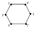
Therefore the results in this section are of a weaker flavor than Theorem 2 since we need to assume that the networks are lossless and we only consider voltage constraints. The results here are useful since in practice some distribution networks consists of a ring feeder and trees hanging of the feeder nodes as in Figure 5.

In this case, the objective functions are often to minimize the loss at the feeders. Also, the feeder nodes are generally considered as slack buses, so they only have a voltage constraint. Since minimizing a linear function over and has the same objective values, characterizing the convex hull of the injection region is useful.
The voltage constraint injection region is defined as
| (18) |
We can again define a enlarged convex region as
| (19) |
We have the following theorem
Theorem 5.
The next theorem states that joining the basic types of networks in a certain way preserves the characterization result. Given two networks and , the network is said to be a 1-connection of and if it is possible to decompose into two components and such that they have only one node in common and no edges between them, where is equal to and is equal to . Note by equal we mean that the admittance matrices are identical. In particular, if a line in or is lossless then its corresponding line in is also lossless. We say is obtained by 1-connecting and . Figure 5 gives an example of a network obtained by 1-connecting a cycle and a number of trees.
Theorem 6.
Given a network on nodes with voltage constraints. Then if the network is a result of repeatedly 1-connecting a lossless cycle and a tree.
It is simple to check if a network has the topology that satisfies the conditions in Theorem 6. Given a network, first decompose it into its one connected parts which can be done in linear time. Then one simply check each of the parts to see if they are a tree or a lossless cycle.
First we prove Theorem 5. This requires that we prove an analogous result about trees first. Consider the following lemma
Lemma 7.
Proof:
To prove this theorem, it suffices to prove that minimizing linear functions over and has the same optimal objective value for all coefficients [21]. So consider the optimization problem
| (20) | ||||
| subject to | ||||
and its relaxation
| (21) | ||||
| subject to | ||||
where the costs can be general (no longer constraint to be positive). We show for all ’s.
The dual of (21) is
| (22) | ||||
| subject to |
From Lemma 4 if the costs are such that is connected, then the optimal solution to (21) is rank and clearly . If is disconnected, then can be written as a block diagonal matrix. Suppose there are connected components of , then . Since the network is a tree, fits the topology of a tree for each . Then (21) and (22) decomposes into independent primal-dual subproblems, and we may apply Lemma 4 to each of them. Let denote the optimal solutions to each of the subproblems. By Lemma 4, they are all rank so we can write for each . An optimal solution to the original problem is given by where . ∎
Now we prove Theorem 5. The approach is the same as in the proof of Lemma 7. That is, we look at (20), (21) and their dual (22). We say a matrix is lossless if all the off diagonal terms of are purely imaginary or . We prove the following lemma
Lemma 8.
Given a graph on nodes that is either an odd cycle or a cycle with one chord, if is lossless, positive semidefinite and fits , then .
Theorem 5 can be proved from Lemma 8. Suppose the electrical network is lossless and has the topology of an odd cycle or a cycle with one chord. The network being lossless means is purely imaginary, and is also purely imaginary since is real. Suppose that the costs are such that if is connected by a line in the network. Since is diagonal, the dual matrix is positive semidefinite, lossless and fits the network topology. Apply Lemma 8 shows is rank 1. If the cycle is even, we add a chord between two buses, and let the admittance of that chord go to . Since all the functions in (21) are continuous, the optimal solution of the network with a chord approaches the network without the chord as the admittance goes to .
If the costs are such that even if is connected in the network, then either fits a tree or becomes disconnected. If fits a tree, then apply Lemma 4. If becomes disconnected, then can be written as a block diagonal matrix. If there are connected components of , then . Since the network is a cycle (with a chord), then is either a tree or a cycle for each . We can apply Lemma 4 or Lemma 8 to each component and obtain an optimal solution in the same way as in the tree network case. To finish Theorem 5, it remains to proof Lemma 8.
Proof:
Given a graph , the tree-width of is a number that intuitively captures how close is to a tree. For example, the tree-width of a tree is , and the tree-width of a cycle is . The rigorous definition and some methods of computing the tree-width the reader may consult [24]. A graph of tree-width 2 is also called serial-parallel graph or a partial-2-tree. The following lemma collects the known results that we need.
Lemma 9.
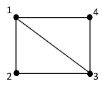
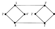
Given a graph with nodes and edges. We construct a bipartite graph derived from that we call the bipartite expansion of and denote by . is a bipartite graph with nodes and edges. Label the nodes with the bipartition being and . There is an edge between and if and only if and is an edge in . If is an odd cycle then is also a cycle and if is a cycle with a chord then has tree-width 2 (a subclass of linear-2-trees in the language of [26]). Two examples are given in Figures 6 and 7. If is an even cycle then is two disconnected cycles, therefore the assumption of odd cycle is needed in the Lemma.

Given a graph , suppose is lossless, positive semidefinite and fits . We show that the rank of cannot be lower than . Suppose has rank . Then can be factored as for some complex matrix matrix . Let be the columns of . They satisfy the graph topology condition
| (23) |
and the lossless line condition
| (24) |
From each complex vector we define two real vectors as
Since , then . By algebra, and . In terms of ’s and ’s, (23) becomes
| (25) |
and (24) becomes
| (26) |
Define the matrix to be the matrix with columns . By (25) and (26) fits . But if is an odd cycle or a cycle with one chord, applying Lemma 9 to gives . Thus or . ∎
Now we proceed to the proof Theorem 6. Given a network , we say the matrix satisfies if fits the topology of and is purely imaginary if the line from bus to bus is lossless. We have the following lemma.
Lemma 10.
Given two networks and with and buses respectively, let be a network obtained by 1-connecting and , so has buses. If is a positive semidefinite matrix that satisfies , then .
From the basic topologies in Theorem 5, we can apply the Lemma 10 repeatedly to get Theorem 6. A version of Lemma 10 just about graphs (without considering lossless lines and such) is known in the graph theory community [25, 27]. We give a proof here to show the additional condition of lossless lines does not change the result.
Proof:
Let , and be networks given in the statement of the Lemma. Label the buses in to be where the subnetwork induced by corresponds to and the subnetwork induced by corresponds to . So bus is the common bus in the 1-connection. Suppose is a positive semidefinite matrix that satisfies and has rank . Then it is possible to factor as for some matrix . Let be the columns of . Let be the subspace spanned by and be the subspace spanned by . By construction of , there are no lines between the set of buses and . Therefore is orthogonal to . We may write vector as where , and is orthogonal to and . Let be the matrix with columns and be the matrix with columns . Let . Since for , equals the matrix formed by the first rows and columns of . By the assumption satisfies , so satisfies . Similarly satisfies . By the assumption in the Lemma, we have and , so equivalently and . Since is orthogonal to and spans , . ∎
[Proof of Theorem 1] The following basic lemma from linear algebra is useful.
Lemma 11 (Rank Nullity Theorem).
Let be a real symmetric matrix. Let and denote the image and kernel of , respectively. Then and , where is the direct sum.
First consider the case where the network is lossless. Then any feasible injection vector must be on the conservation of energy plane. We need to show that any point on the plane can be achieved. Since the network is lossless where is a real symmetric matrix and each row of sums to by (1). Therefore is a generalized graph Laplacian matrix where the admittances can be interpreted as weights on the edges. By a standard result in graph theory, and is spanned by the all one’s vector . By Lemma 11, is the linear subspace in orthogonal to . Let be an injection vector on the conservation of energy plane, that is . Since , there is a unique vector such that and . Choose the voltage vector , then
| (27) | |||
| (28) | |||
where follows from the choice of and being symmetric. This finishes the proof for a lossless network.
Next consider the case where the network is lossy. The proof proceeds in two parts, first we show that the conservation of energy boundary can be arbitrarily closely from above, and then we show the injection region is convex. Since the network is lossy, is a real positive semidefinite Laplacian matrix. By conservation of energy, any power injection vector achieved must satisfy if . Let be a vector on the conservation of energy plane. We show there is a voltage vector that achieves a point arbitrarily close to . Since , by Lemma 11 there is a unique vector such that and . Let for some and the corresponding injection vector is
| (29) | ||||
where follows from and is symmetrical, follows from the choice of . We can increase to make arbitrarily close to . For example, if we want , then choose
The next lemma states that is convex.
Lemma 12.
The injection region as defined in eqn. (5) is a convex set.
Theorem 1 follows from Lemma 12. Since the injection region is convex, and the boundary can be approached arbitrarily closely from above, it includes the open half upper space. In addition the origin can be achieved using the all zeros voltage vector. It remains to prove the lemma.
Proof:
For a given network with buses represented by , define as
| (30) |
where . approaches the unconstrained injection region as tends to infinity. cannot have holes since if , then for . Therefore to prove the convexity of it suffices to prove it has convex boundary. Consider the optimization problem
| (31) | ||||
| subject to | ||||
Relaxing and eliminating , we get
| (32) | ||||
| subject to | ||||
By changing the costs, we are exploring the boundaries of the two regions with linear functions. We want to show that all the point on the boundary of the larger region is in fact in the smaller region.
First we show that for all there is an optimal for (32) which is rank 1. To solve (32), expand in terms of its eigenvectors, so where is unit norm and . Then (32) can be written as
| minimize | (33) | |||
| subject to | ||||
By the well known result about Rayleigh quotients [28], to minimize any of the terms , the optimal , where is the eigenvector corresponding to the smallest eigenvector of . Therefore the optimal solution to (32) is and is rank 1.
If is not unique, since eigenvector are not continuous in the entries of the matrix, we can perturb by an arbitrarily small amount to obtain a that has a unique eigenvector corresponding to the smallest value. Note the power vector is continuous in the entries of . From uniqueness of and the fact there is no gap between (31) and (32), the two regions have the same boundary. Taking to infinity finishes the proof. ∎
References
- [1] B. Stott, O. Alsac, and A. J. Monticelli, “Security analysis and optimization,” Proceedings of the IEEE, 1987.
- [2] H. W. Dommel and W. F. Tinney, “Optimal power flow solutions,” IEEE Transactions on Power Apparatus and Systems, 1968.
- [3] R. V. Amarnath and N. V. Ramana, “State of the art in optimal power flow solution methodologies,” Journal of Theoretical and Applied Information Technology, vol. 30, no. 2, pp. 128–154, 2011.
- [4] T. J. Overbye, X. Cheng, and Y. Sun, “A comparison of the AC and DC power flow models for lmp calculations,” in Proceedings of the 37th Hawaii International Conference on System Sciences, 2004.
- [5] B. Stott, J. Jardim, and O. Alsac, “DC power flow revisited,” IEEE Transactions on Power Systems, 2009.
- [6] J. Lavaei and S. Low, “Zero duality gap in optimal power flow,” To appear in IEEE Transactions on Power Systems, 2011.
- [7] Y. V. Makarov, Z. Y. Dong, and D. J. Hill, “On convexity of power flow feasibility boundary,” IEEE Transactions on Power Systems, 2008.
- [8] B. Lesieutre, D. Molzahn, A. Borden, and C. L. DeMarco, “Examining the limits of the application of semidefinite programming to power flow problems,” in Allerton 2011, 2011.
- [9] M. Albadi and E. El-Saadany, “Demand response in electricity markets: an overview,” in Proceedings of the IEEE Power Engineering Society general meeting, 2007.
- [10] US Department of Energy, “Benefits of demand response in electricity markets and recommendations for achieving them,” A report to the United States congress, 2006.
- [11] G. R. Oapos and M. A. Redfern, “Voltage control problems on modern distribution systems,” in Proceedings of the IEEE Power Engineering Society general meeting, 2004.
- [12] B. C. Lesieutre and I. A. Hiskens, “Convexity of the set of feasible injections and revenue adequacy in ftr markets,” IEEE Transactions on power systems, 2005.
- [13] W. Hogan, “Contract networks for electric power transmission: Technical reference,” http://ksghome.harvard.edu/~whogan/acnetref.pdf, 1992.
- [14] J. Lavaei, “Competitive equilibria in electricity markets with nonlinearities,” Submitted to IEEE Transactions on Power Systems, 2011.
- [15] S. Sojoudi and J. Lavaei, “Network topologies guaranteeing zero duality gap for optimal power flow problem,” Submitted to IEEE Transactions on Power Systems, 2011.
- [16] S. Bose, D. F. Gayme, S. Low, and M. K. Chandy, “Optimal power flow over tree networks,” Proceedings of the Forth-Ninth Annual Allerton Conference, pp. 1342–1348, 2011.
- [17] W. H. Kersting, Distribution system modeling and analysis. CRC Press, 2006.
- [18] J. Jarjis and F. Galiana, “Quantitative analysis of steady state stability in power systems,” IEEE Trans. Power App. Syst., 1981.
- [19] J. W. Helton and A. Vityaev, “Analytic functions optimizing competing constraints,” SIAM J. Math. Anal., vol. 28, no. 3, pp. 749–767, 1997.
- [20] R. Baldick, Applied Optimization: Formulation and Algorithms for Engineering Systems. Cambridge, 2006.
- [21] S. Boyd and L. Vandenberghe, Convex Optimization. Cambridge, 2004.
- [22] H. van der Holst, “Graphs whose positive semi-definite matrices have nullity at most two,” Linear Algebra and its Applications, 2003.
- [23] Distribution Test Feeder Working Group, “Distribution test feeders,” http://ewh.ieee.org/soc/pes/dsacom/testfeeders/index.html, 2010.
- [24] H. L. Bodlaender, “A linear time algorithm for finding tree-decompositions of small treewidth,” SIAM Journal on Computing, 1996.
- [25] S. M. Fallat and L. Hogben, “The minimum rank of symmetric matrices described by a graph: A survey,” Linear Algebra Applications, 2007.
- [26] C. R. Johnson, R. Loewy, and P. A. Smith, “The graphs for which the maximum multiplicity of an eigenvalue is two,” Linear and Multilinear Algebra, 2009.
- [27] J. Beagley, E. Radzwion, S. Rimer, R. Tomasino, J. Wolfe, and A. Zimmer, “On the minimum semidefinite rank of a graph using vertex sums, graphs with , and the msrs of certain graph classes,” NSF-REU report from Central Michigan University, 2007.
- [28] R. A. Horn and C. A. Johnson, Matrix Analysis. Cambridge, 1985.