Stochastic treatment of finite-$N$ effects in mean-field systems and its application to the lifetimes of coherent structures

Abstract

A stochastic treatment yielding to the derivation of a general Fokker-Planck equation is presented to model the slow convergence towards equilibrium of mean-field systems due to finite-$N$ effects. The thermalization process involves notably the disintegration of coherent structures that may sustain out-of-equilibrium quasistationary states. The time evolution of the fraction of particles remaining close to a mean-field potential trough is analytically computed. This indicator enables to estimate the lifetime of coherent structures and thermalization timescale in mean-field systems.

Many physical systems may be considered as isolated assemblies of $N$ bodies interacting via long-range pair interactions. This is the case for systems ranging from charged particles interacting via Coulomb interaction to self-gravitating massive objects like globular clusters or stars in galaxies and this may even include suitably prepared Bose-Einstein condensates ODell in a close future. The physically relevant issue of the dynamics of those systems in the large-$N$ limit forms the subject of kinetic theory. Long-range systems are prone to collective behavior that may be largely dominating before binary collisional effects set on. This hierarchy between collective and collisional behavior is responsible for the unusual properties of the relaxation process towards equilibrium as well as for the richness and complexity of the physics of long-range systems. These are motivations for the present considerable interest raised by long-range systems in various fields such as plasma physics, astrophysics Gabrielli2010 , statistical physics Campa or applied mathematics.

Collective behavior of long-range systems as well as the intricacies of the relationships between their dynamics, kinetic theory and equilibrium statistical properties may be more conveniently unveiled through models that are already of mean-field type for finite $N$. These are Hamiltonian models describing e.g. wave-particle interaction ElskensEscande , which is an ubiquitous phenomenon in hot and dilute plasmas, or the all-to-all coupling of $N$ bodies in long-range interactions of the kind of gravitation in a compact space AntoniRuffo ; EttFir . Despite their relative simplicity, such models develop a rich long-range phenomenology. This includes in particular the emergence of quasistationary states (QSSs) having lifetimes diverging with $N$, during which the time average of macroscopic quantities, such as the temperature or the modulus of mean-fields, differs from their equilibrium statistical mechanics ensemble averages. These QSSs may be connected to the existence of coherent structures that may be viewed as long-lived phase space patterns related to locally insufficient mixing properties CoherentFH . Consequently, the relaxation to equilibrium should accompany the disintegration of coherent structures.

The Letter is organized as follows: first, a stochastic treatment of finite $N$-effects in mean field systems will be proposed leading to the establishment of a Fokker-Planck equation. In order to test this model, we then shall consider an Hamiltonian model of $N$ particles in self-consistent interaction via a cosine potential. Starting from configurations where $\mathcal{O}(N)$ particles are trapped into their self-potential well, an analytic expression giving the fraction of the particles that remain trapped as a function of time will be successfully tested against numerical results. The relevance of this indicator to the thermalization issue will be shortly discussed.

Consider $N$ particles evolving in the phase space $S_{L}^{N}\times\mathbb{R}^{N}$ under the dynamics deriving from the Hamiltonian

$$\mathcal{H}=\sum\limits_{i=1}^{N}{\mathchoice{\dfrac{{p_{i}}^{2}}{2}}{\dfrac{{p_{i}}^{2}}{2}}{\frac{{p_{i}}^{2}}{2}}{\frac{{p_{i}}^{2}}{2}}}+{\mathchoice{\dfrac{1}{2N}}{\dfrac{1}{2N}}{\frac{1}{2N}}{\frac{1}{2N}}}\sum\limits_{n=1}^{s}\sum\limits_{i,j=1}^{N}V_{n}\cos\left[k_{n}(q_{j}-q_{i})\right],$$ (1)

where $q_{i}\in S_{L}$ is the position of particle $i$ on the circle $S_{L}\equiv\mathbb{R}/L$, $p_{i}$ its conjugate momentum, and where only the first $s$ long-range components with wave numbers $k_{n}=2\pi n/L$, for $1\leq n\leq s$, are retained in the potential term. When $V_{n}\propto n^{-2}$, model (1) amounts to the long-range truncation of the one-dimensional Newtonian potential with space-periodic boundary conditions, that describes Coulomb or gravitational interaction depending on the potential sign. Various systems covered by (1) have been discussed in Ref. Elskens . An extension to a spatial dimension $d>1$ should not be a conceptual problem. Introducing the set of collective observables $\{\mathbf{M}_{n}\}$ through

$$\mathbf{M}_{n}={\mathchoice{\dfrac{1}{N}}{\dfrac{1}{N}}{\frac{1}{N}}{\frac{1}{N}}}\sum\limits_{j=1}^{N}\left(\cos(k_{n}q_{j}),\sin(k_{n}q_{j})\right)=M_{n}(\cos\phi_{n},\sin\phi_{n})$$ (2)

yields the equation of motion of any particle $i$ as

$$\ddot{q}_{i}+\sum\limits_{n=1}^{s}k_{n}V_{n}M_{n}\sin(k_{n}q_{i}-\phi_{n})=0.$$ (3)

Therefore, the collective variables $M_{n}$ behave as mean fields that, as well as the phases $\phi_{n}$, depend on time through the self-consistency relations (2).

For smooth potentials like in (1), the convergence of the finite-$N$ dynamics to Vlasov equation is rigorously proved on arbitrary finite-time intervals Spohn . Vlasov equation being time reversible, its solution $f(p,q,t)$ cannot approach an equilibrium VanKampen , yet macroscopic quantities, involving phase space integrals of $f$, such as the mean-fields, can converge to stationary values associated to QSSs. In the realistic finite-$N$ Hamiltonian framework, finite-$N$ effects will in the long term induce the thermalization process and disintegration of coherent structures possibly sustaining those QSSs.

Modelling this process, we assume that the system (1) is trapped in a QSS, such that one can write the mean fields as $M_{n}(t)=M_{n}^{0}(t)+\delta M_{n}(t)$ with $\delta M_{n}\ll M^{0}_{n}$, where $\delta M_{n}$ varies on a time scale which is very much smaller than the characteristic time scale of $M_{n}^{0}$, the latter being comparable to a local average. We now make the hypothesis that during the QSS regime, the fluctuations around the local mean value have a variance decreasing as $N^{-1}$. The central idea behind this is to replace the deterministic but yet very chaotic fluctuations of $\delta M_{n}$ by stochastic processes, whose variances are suitably chosen. Numerical observations support this modeling. For instance, as shown in Fig. 1 for some special case, the mean fields clearly exhibit two different timescales, in agreement with the decomposition suggested earlier. Moreover, both histograms and the autocorrelation function shown in Fig. 1 suggest that one can model the fluctuations $\delta M_{n}$ by a Gaussian (white) noise.

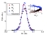
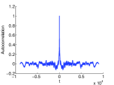
Figure 1: (Left) Comparison between the numerically computed fluctuations of $M_{1}$, $M_{2}$ and $M_{3}$ around their local average $\left\langle M_{n}\right\rangle$ with a Gaussian fit, for system (1) with $s=3$ and $V_{n}=n$ starting from an arbitrary initial condition. The inset shows the evolution of $M_{1}$, $M_{2}$ and $M_{3}$ with respect to time. (Right) Autocorrelation of $M_{1}$ after subtracting its local average.

Replacing $\delta M_{n}$ by the noise $\xi_{n}$ such that $\left\langle\xi_{n}\right\rangle$=0, and $\left\langle\xi_{n}(t)\xi_{n}(t^{\prime})\right\rangle\propto N^{-1}\delta(t-t^{\prime})$, the Fokker-Planck equation (FPE) associated to the Langevin equations coming from the stochastic version of the equations of motion (3) reads

$${\mathchoice{\dfrac{\partial f}{\partial t}}{\dfrac{\partial f}{\partial t}}{\frac{\partial f}{\partial t}}{\frac{\partial f}{\partial t}}}+{\mathchoice{\dfrac{\partial}{\partial q}}{\dfrac{\partial}{\partial q}}{\frac{\partial}{\partial q}}{\frac{\partial}{\partial q}}}\left(pf\right)-\sum\limits_{n=1}^{s}k_{n}V_{n}M^{0}_{n}\sin(k_{n}q-\phi_{n}){\mathchoice{\dfrac{\partial f}{\partial p}}{\dfrac{\partial f}{\partial p}}{\frac{\partial f}{\partial p}}{\frac{\partial f}{\partial p}}}\\ =\sum\limits_{n=1}^{s}{\mathchoice{\dfrac{{k_{n}}^{2}{V_{n}}^{2}}{2}}{\dfrac{{k_{n}}^{2}{V_{n}}^{2}}{2}}{\frac{{k_{n}}^{2}{V_{n}}^{2}}{2}}{\frac{{k_{n}}^{2}{V_{n}}^{2}}{2}}}\left\langle{\xi_{n}}^{2}\right\rangle\sin^{2}(k_{n}q-\phi_{n}){\mathchoice{\dfrac{\partial^{2}f}{\partial p^{2}}}{\dfrac{\partial^{2}f}{\partial p^{2}}}{\frac{\partial^{2}f}{\partial p^{2}}}{\frac{\partial^{2}f}{\partial p^{2}}}}$$ (4)

This equation may be interpreted as a Vlasov equation supplemented with a r.h.s. of order $N^{-1}$, consistently with the argument presented in Ref. Campa , coming here not from binary collisions but from the fluctuations of the mean fields. This differs from other FPEs derived in mean-field systems in other places BouchetDauxois2005 ; Chavanis2010 . Moreover, this equation was derived without any need to invoke dissipation (see e.g. Mallick ).

In what follows, we shall consider the case of a single resonance ($s=1$) in which coherent structures may survive for long times close to the potential trough (see e.g. Fig. 2). The FPE (4) may be further simplified by looking for solutions in separate variables $q$ and $p$ writing $f(p,q,t)=g(q,t)\tilde{f}(p,t)$. Assuming that $g$ is even in the wave frame and that $\int_{0}^{L}g(q,t)\mathrm{d}q$ is constant, one obtains a simple diffusion equation

$${\mathchoice{\dfrac{\partial\tilde{f}}{\partial t}}{\dfrac{\partial\tilde{f}}{\partial t}}{\frac{\partial\tilde{f}}{\partial t}}{\frac{\partial\tilde{f}}{\partial t}}}=\mathcal{D}(t){\mathchoice{\dfrac{\partial^{2}\tilde{f}}{\partial p^{2}}}{\dfrac{\partial^{2}\tilde{f}}{\partial p^{2}}}{\frac{\partial^{2}\tilde{f}}{\partial p^{2}}}{\frac{\partial^{2}\tilde{f}}{\partial p^{2}}}},$$ (5)

with diffusion coefficient

$$\mathcal{D}(t)={\mathchoice{\dfrac{{k}^{2}{V}^{2}}{2}}{\dfrac{{k}^{2}{V}^{2}}{2}}{\frac{{k}^{2}{V}^{2}}{2}}{\frac{{k}^{2}{V}^{2}}{2}}}\left\langle{\xi}^{2}\right\rangle\overline{\sin^{2}(kq-\phi)},$$ (6)

and $\overline{\sin^{2}(kq-\phi)}\equiv\int_{0}^{L}\sin^{2}(kq-\phi)g(q,t)\mathrm{d}q/\int_{0}^{L}g(q,t)\mathrm{d}q$. Numerical evidence Campa supports the fact that $p$ and $q$ may be treated as separate variables and that $q$ may be considered as a fast variable compared to $p$, meaning that the distribution function in $q$ approaches much more quickly its Boltzmann-Gibbs shape than the $p$ one consistently with basic dimensional arguments Mallick . The forthcoming numerical tests will show that the average of $\sin^{2}(kq-\phi)$ may be effectively replaced by its ensemble average.

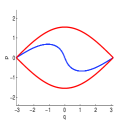
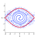
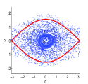
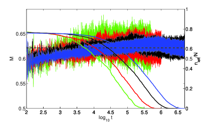
Figure 2: (Upper panel) Phase-space snapshots at increasing times (from left to right, $t=6$, $t=100$ and $t=2000$) for an initial cold-beam condition of energy $U=0.5$. The simulation was performed using $N=10^{4}$ particles.The instantaneous separatrix is plotted in bold red. (Lower panel) Time evolution of the magnetization $M$ and fraction $n_{\ell}/N$ for $N=10^{3}$ (green), $2.10^{3}$ (red), $5.10^{3}$ black and $10^{4}$ (blue) particles.

From now on, in order to simplify expressions, we shall put $V=1$ and $L=2\pi$, which gives $k=1$. This amounts to the well-known Hamiltonian Mean Field model Campa . Figure 2 shows numerical results obtained starting from a monokinetic beam EttFir . The upper panel shows the one-particle phase space plots at three different stages of the evolution. Deep inside the mean-field potential trough, particles move almost regularly forming a clear coherent structure pattern that progressively dissipates. It is interesting to note the similarity of these figures with the phase space plots for the 1-D finite-$N$ cold dark matter simulations of Ref. Binney2004 . The lower panel shows the evolution of the mean-field for four different numbers of particles, ranging from $N=10^{3}$ to $N=10^{4}$. The dashed line marks its equilibrium ensemble average. It is clear from the figure that the convergence towards equilibrium slows down as $N$ increases. Also displayed is the evolution of $n_{\ell}/N$, that is the fraction of particles initially trapped within the separatrices and which remain inside them up to time $t$. During a short transient regime (not shown), about twenty percent of the particles escape the mean-field resonance. It is only after this lapse of time that the regime becomes diffusive. Most importantly, Fig. 2 gives an evidence that the cancelation time of $n_{\ell}/N$ may be used as a marker of thermalization as it qualitatively coincides with the time where the mean-field begins to fluctuate around its equilibrium value in a stable way. This is not surprising since, at the time when $n_{\ell}/N$ vanishes, the coherent structure has been completely disintegrated. The dependence of $M$ on $N$ becomes much clearer when increasing $N$ to values of the order of $10^{5}$, but the numerical cost was too important for us to perform a full simulation leading to a vanishing $n_{\ell}/N$. However, the early-time behaviour of $n_{\ell}/N$ was still correctly described by our model.

The equations of the separatrices are given by $p_{S}(t)=\pm 2\sqrt{M(t)}\cos(q/2)$. Let us put $\lambda=2\sqrt{M^{0}}$ and consider it to be almost constant. Figure 2 is a motivation to answer the following question: What is the number of particles $n_{\ell}(t)$, having initially momenta comprised between $-\lambda$ and $\lambda$, that remain in this domain up to time $t$ ? Among such particles are the particles forming the core of coherent structures that slow down the mixing process. However, because of the parametric resonance induced by the mean fields fluctuations, these particles will eventually escape, and we shall now estimate the characteristic time needed by the system to evacuate a fraction $1-\delta$ of the $N_{0}$ particles initially contained in the band of momenta $[-\lambda;\lambda]$. Using the linearity of the diffusion equation (5), one can focus on the contribution of particles whose momenta remain up to time $t$ within the band $[-\lambda;\lambda]$ and solve (5) by imposing the cancelation of $f$ at $p=\pm\lambda$. Finally, integrating over $p$ yields the solution

$$\frac{n_{\ell}(t)}{N_{0}}=\sum\limits_{n=0}^{\infty}{\mathchoice{\dfrac{2(-1)^{n+1}c_{n}}{(2n+1)\pi}}{\dfrac{2(-1)^{n+1}c_{n}}{(2n+1)\pi}}{\frac{2(-1)^{n+1}c_{n}}{(2n+1)\pi}}{\frac{2(-1)^{n+1}c_{n}}{(2n+1)\pi}}}\mathrm{exp}\left(-{\mathchoice{\dfrac{(2n+1)^{2}\pi^{2}}{4\lambda^{2}}}{\dfrac{(2n+1)^{2}\pi^{2}}{4\lambda^{2}}}{\frac{(2n+1)^{2}\pi^{2}}{4\lambda^{2}}}{\frac{(2n+1)^{2}\pi^{2}}{4\lambda^{2}}}}\mathcal{D}t\right),$$ (7)

with $\mathcal{D}$ given by Eq. (6) and

$$c_{n}=\frac{\int_{-\lambda}^{\lambda}\tilde{f}(p,t=0)\cos\left(\frac{(2n+1)p\pi}{2\lambda}\right)\mathrm{d}p}{\int_{-\lambda}^{\lambda}\tilde{f}(p,t=0)\mathrm{d}p}.$$ (8)

As confirmed by the numerical simulations shown in Fig. 3, the dynamics arising from Eq. (5) proves to correctly depict the escape process through the validation of Eqs. (7)-(8). In these numerical simulations, particles were initially distributed according to a so-called waterbag distribution

$$f_{0}(p,q)=\Theta(\Delta p-|p|)\Theta(\Delta q-|q|)/(4\Delta p\Delta q)$$ (9)

where $\Theta$ stands for the Heaviside step function. It is interesting to note that when starting from these initial waterbag conditions, the phase-space distribution eventually exhibits a core-halo structure, which has been recently investigated in Pakter2011 .

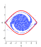
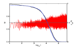
Figure 3: (Left) Snapshot of the one-particle phase space at $t=12$ for $N=5000$ particles initially distributed in a waterbag configuration (9) with $\Delta p=0.848$ and $\Delta q=2.16$. (Right) Time evolution of the mean-field $M$ (red curve) and of $n_{l}/N$ (black curve). The blue dashed curve is the analytic expression for $n_{\ell}/N$ as deduced from Eqs. (7)-(8). The initial time has been chosen at time $t=10$ and $N_{0}=0.95N$.

Once again, it is visible on Fig. 3 that, at the time when all the particles that where initially in the momentum band $[-\lambda;\lambda]$ have at least once escaped this domain, the system has seemingly reached its thermal equilibrium. In order to test the escape model given by Eqs. (7)-(8), one needs to know the diffusion coefficient $\mathcal{D}$ given by Eq. (6). As already discussed, $\overline{\sin^{2}(q)}$ may be estimated from $\left\langle\sin^{2}q\right\rangle_{c}=I_{1}\left(\beta\left\langle M\right\rangle_{c}\right)/[\beta\left\langle M\right\rangle_{c}I_{0}\left(\beta\left\langle M\right\rangle_{c}\right)]$. A priori $\langle\xi^{2}\rangle$ has to be determined from numerical simulations since the system is not at equilibrium. However, in the cases that were considered, the numerically computed variance $\langle\xi^{2}\rangle$ was almost indistinguishable from its canonical value given by

$$\left\langle\delta^{2}M\right\rangle_{c}={\mathchoice{\dfrac{2}{N}}{\dfrac{2}{N}}{\frac{2}{N}}{\frac{2}{N}}}{\mathchoice{\dfrac{\partial}{\partial\beta}}{\dfrac{\partial}{\partial\beta}}{\frac{\partial}{\partial\beta}}{\frac{\partial}{\partial\beta}}}\log\left[{\mathchoice{\dfrac{v^{*}}{\beta}}{\dfrac{v^{*}}{\beta}}{\frac{v^{*}}{\beta}}{\frac{v^{*}}{\beta}}}\sqrt{{\mathchoice{\dfrac{2\pi N}{\partial^{2}_{v}\psi|_{v^{*}}}}{\dfrac{2\pi N}{\partial^{2}_{v}\psi|_{v^{*}}}}{\frac{2\pi N}{\partial^{2}_{v}\psi|_{v^{*}}}}{\frac{2\pi N}{\partial^{2}_{v}\psi|_{v^{*}}}}}}\mathrm{e}^{-N\psi(v^{*})}\right]-{\mathchoice{\dfrac{{v^{*}}^{2}}{\beta^{2}}}{\dfrac{{v^{*}}^{2}}{\beta^{2}}}{\frac{{v^{*}}^{2}}{\beta^{2}}}{\frac{{v^{*}}^{2}}{\beta^{2}}}},$$ (10)

where $\psi(v)=v^{2}/(2\beta)-\log I_{0}(v)$ and $v^{*}=\beta\left\langle M\right\rangle_{c}$ satisfies the self-consistency equation $\partial_{v}\psi|_{v^{*}}=0$. Numerically, this gives $\left\langle\xi^{2}\right\rangle\approx 0.43/N$, which is consistent with the fit obtained from numerical simulations. As shown in Fig. 3, the agreement between the numerically computed time evolution of $n_{\ell}/N$ and its analytic modeling (7)-(8) is quite satisfactory.

Let us finally estimate the time needed to destroy the inner coherent structure by the means of Eq. (7). Considering that $N_{0}=\mathcal{O}(N)$ and $\mathcal{D}=\mathcal{O}(N^{-1})$, a rough estimate of the time $\tau_{\delta}(N)$ needed for $n_{\ell}/N$ to reach down a sufficiently small fraction $\delta$ gives

$$\tau_{\delta}(N)\propto-N\log\delta.$$ (11)

When $\mathcal{D}$ depends on time, Eq. (11) follows from the mean value theorem. This first result recovers the linear $N$ scaling found in the abundant literature of long-range interacting systems AntoniRuffo ; Joyce ; Chavanis , where the numerical evidence is extracted from thresholds equivalent to the $\delta$ criterion imposed here. One does not expect the continuum approach behind Eq. (7) to remain valid for vanishingly small values of $\delta$. However, going up to the limit of validity of this model, one may infer that the sweeping of phase space is sufficient to reach a complete thermalization at a time $\tau_{QSS}$ when $n_{\ell}=\mathcal{O}(1)$. Then Eq. (11) would give the maximal scaling $\tau_{QSS}\propto N\log N$. This corresponds to the scaling recently suggested in Ref. Gupta for the $s=1$ case.

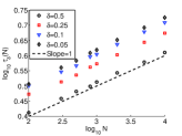
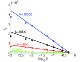
Figure 4: (Left) Plot of $\tau_{\delta}(N)$ in log-log scale with respect to $N$. As predicted by Eq. (11), the behavior is linear with $N$. (Right) Plot of the numerically measured $\tau_{\delta}$ with respect to $\log\delta$. The behavior is linear over a wide range of $\delta$. As expected, the measured times for very low threshold values are lower than the logarithmic prediction of Eq. (11), since the latter is obtained in the continuous limit.

Eq. (11) predicts a linear behavior with respect to $N$, which we found to be correct over the whole range of values of $N$ studied here, independently from the chosen threshold $\delta$. We also checked the scaling with the latter parameter. Figure 4 shows a very good agreement between Eq. (11) and the numerical simulations.

These scalings contrast with the numerically obtained $N^{1.7}$ scaling for the QSS lifetime starting from two special initial conditions Zanette2003 ; Yamaguchi . These cases are however not in contradiction with the results presented here since, even this is less obvious for Zanette2003 , they both correspond to QSS about a vanishing mean-field, a case that is excluded from the present framework since the phase would be no longer defined. In the intermediate cases, where the QSS magnetization is clearly above zero, but yet far from the equilibrium expectation, this method provides a good estimation of the time needed to destroy the coherent structures, but fails to predict the QSS lifetime, since the effective model does not capture the average growth of the separatrix with time.

The present framework and results are expected to be easily transposable to wave-particle models in which finite-$N$ effects eventually drive the system towards equilibrium in contradiction with the Vlasov approach Firpo01 . This discreteness effect may be more than a numerical concern for simulations since some physical effects YoonPRL2005 cannot be explained in the Vlasov limit.

References

- [1] D. O’Dell et al., Phys. Rev. Lett. 84 5687 (2000).
- [2] A. Gabrielli, M. Joyce, and B. Marcos, Phys. Rev. Lett. 105 210602 (2010).
- [3] Campa A et al., Phys. Rep. 480 57 (2009)
- [4] Y. Elskens, D. Escande, Microscopic dynamics of plasmas and chaos (IoP Publishing, Bristol, 2003).
- [5] M. Antoni, S. Ruffo, Phys. Rev. E 52 2361 (1995)
- [6] W. Ettoumi, M.-C. Firpo, J. Phys. A 44 175002 (2011)
- [7] See e.g. A. K. M. Fazle Hussain, J. Fluid Mech. 173, 303 (1986) for a comprehensive definition of coherent structures in the fluid mechanics context.
- [8] Y. Elskens, M. Antoni, Phys. Rev. E 55 6575 (1997)
- [9] H. Spohn, Large Scale Dynamics of Interacting Particles (Springer, Berlin, 1991).
- [10] N.G. Van Kampen, B.U. Felderhof, Theoretical methods in plasma physics (North-Holland, Amsterdam, 1967).
- [11] F. Bouchet, T. Dauxois, Phys. Rev. E 72, 045103(R) (2005)
- [12] P.H. Chavanis, J. Stat. Mech. (2010) P05019.
- [13] K. Mallick, P. Marcq, J. Phys. A: Math. Gen. 37 4769 (2004)
- [14] J. Binney, Mon. Not. R. Astron. Soc. 350, 939 (2004)
- [15] M. Joyce, T. Worrakitpoonpon, J. Stat. Mech. P10012 (2010)
- [16] P.-H. Chavanis, Physica A 361 81 (2006)
- [17] S. Gupta, D. Mukamel, Phys. Rev. Lett. 105 040602 (2010)
- [18] R. Pakter, Y. Levin, accepted in Phys. Rev. Lett. (2011)
- [19] D.H. Zanette, M.A. Montemurro, Phys. Rev. E 67, 031105 (2003)
- [20] Y. Yamaguchi et al., Physica A 337 36 (2004)
- [21] M.-C. Firpo et al., Phys. Rev. E 64, 026407 (2001)
- [22] P. H. Yoon, T. Rhee, and C.-M. Ryu, Phys. Rev. Lett. 95, 215003 (2005)