Simplicial gauge theory on spacetime

Abstract.

We define a discrete gauge-invariant Yang-Mills-Higgs action on spacetime simplicial meshes. The formulation is a generalization of classical lattice gauge theory, and we prove consistency of the action in the sense of approximation theory. In addition, we perform numerical tests of convergence towards exact continuum results for several choices of gauge fields in pure gauge theory.

1. Introduction

This article is the natural prolongation of an earlier work [2]. In [2] we defined a gauge invariant discrete action to approximate the Yang-Mills-Higgs (YMH) action [17, 13, 14, 12] on a simplicial mesh approximation of a spatial domain, and we proved consistency of the discrete action for smooth fields. In this article we expand the discussion to 4d spacetime simplexes in time and three spatial dimensions, and we also expand the consistency proof to fields in the natural energy norm.

More precisely, we define the spatial part of the discrete action as in [2], using Whitney forms [15], Wilson lines and loops [16, 6], and concepts from FEM [5, 9, 10]. We then expand the spatial mesh to spacetime by uniformly discretizing time. The spacetime mesh is defined by repeating the spatial mesh at every time step. Furthermore, we extend the Whitney forms to spacetime, yielding a natural expansion of the discrete spatial action to a spacetime action.

The purpose of this work is to prove consistency of the resulting approximation scheme for the classical YMH equations, and also to develop an analogue of lattice gauge theory, i.e. performing quantum field calculations using the introduced action. The latter will be described in a companion article [8].

We use the same notation as in [2], and the article is organized as follows. In section 2 we introduce the continuous YMH action, and also develop the proposed simplicial gauge theory. In section 3 we review some properties of the differential of the exponential map for matrix groups and the Baker-Campbell-Hausdorff formula. We prove consistency of the action in the energy norm in section 4. Finally, in section 5 we describe some numerical convergence tests, performed on several gauge fields for which the continuum action was exactly calculable.

2. Construction

2.1. The continuous Yang-Mills action

Let $\mathbb{M}=\mathbb{R}\times S$ be a riemannian spacetime manifold, where $\mathbb{R}$ represents time and $S$ is a bounded domain in three dimensional euclidean space. We let $\mathbb{M}$ be equipped with a lorentzian or euclidean signature and coordinates $x=(t,\mathbf{x})$. Furthermore, let $\mathcal{G}$ be a compact Lie group with associated Lie algebra $\mathfrak{g}$, and assume that $\mathcal{G}$ can be represented by a subgroup of the complex unitary $n\times n$ matrices, for some $n$. The hermitian conjugate of a matrix $g$ is denoted $g^{H}$ and the real valued scalar product is

(2.1) $$g^{\prime}\cdot g:=\Re\text{tr}(g^{\prime}g^{H}).$$

The space of smooth $k$-forms on $\mathbb{M}$ is denoted $\Omega^{k}(\mathbb{M})$, and the space $\Omega^{k}(\mathbb{M})\otimes\mathfrak{g}$ can be identified with the space of smooth $\mathfrak{g}$-valued $k$-forms on $\mathbb{M}$. The bracket of Lie algebra valued forms is defined as

(2.2) $$[u\otimes g,u^{\prime}\otimes g^{\prime}]:=(u\wedge u^{\prime})\otimes[g,g^{\prime}],$$

where $u,u^{\prime}$ are real valued differential forms and $g,g^{\prime}\in\mathfrak{g}$.

A connection one-form on $\mathbb{M}$ is an element $\mathbb{A}=(A_{0},A)\in\Omega^{1}(\mathbb{M})\otimes\mathfrak{g}$, where $A_{0}$ represents the time component and $A$ the spatial component. The temporal curvature $\mathcal{F}^{t}(\mathbb{A})$ and spatial curvature $\mathcal{F}^{s}(A)$ of such a one-form are given by

(2.3) $$\mathcal{F}^{t}(\mathbb{A})=dA_{0}+d_{t}A+[A_{0},A],\qquad\mathcal{F}^{s}(A)=dA+\frac{1}{2}[A,A],$$

where $d_{t}$ and $d$ denote exterior derivative in the temporal and spatial direction respectively. We will also use such forms with lower regularity, see e.g. [3]. The independent variable in Yang-Mills theory is such a connection one-form (not necessarily smooth), and the action describing it is given by $S[\mathbb{A}]=S[\mathbb{A}]_{t}+S[A]_{s}$, where

(2.4) $$S[\mathbb{A}]_{t}:=\int_{\mathbb{M}}|\mathcal{F}^{t}(\mathbb{A})|^{2},\qquad S[A]_{s}:=\int_{\mathbb{M}}|\mathcal{F}^{s}(A)|^{2}.$$

A gauge transformation of a connection one-form $\mathbb{A}$ is associated with a choice of $G\in\mathcal{G}$ for each $x\in\mathbb{M}$, such that

(2.5) $$A_{0}(x)\mapsto G(x)\left(A_{0}(x)+d_{t}\right)G^{-1}(x),\qquad A(x)\mapsto G(x)\left(A(x)+d\right)G^{-1}(x).$$

The action $S[\mathbb{A}]$ is invariant under such gauge transformations.

2.2. The interpolated FEM action

In the FEM formulation, we assume $\mathcal{T}$ to be a simplicial complex spanning the spatial domain $S$. The simplexes are referred to as vertexes, edges, faces and tetrahedra according to dimension, and are labeled $i$, $e$, $f$ and $T$ respectively. The symbol $T$ will also be used for simplexes of any dimension. We also suppose an orientation has been chosen for each simplex in $\mathcal{T}$. In addition, we assume that time is discretized with a time step $\Delta t$, and that the simplicial complex $\mathcal{T}$ is repeated at every time step, resulting in a spacetime simplicial complex $\mathbb{T}$. For a more detailed definition of simplicial complexes, consult [4, section 5].

Thus, as the basic building block in classical FEM theory is a tetrahedron $T$, the basic building block in this extended FEM version is $T\times I_{\tau}$, where $I_{\tau}=[\tau,\tau+\Delta t]$ and $\tau$ denotes the temporal nodes.

Furthermore, let $W^{k}(\mathcal{T})$ ($W^{k}(T)$) be the space of Whitney k-forms [15] on $\mathcal{T}$ ($T$), with canonical basis $(\lambda_{T})$, $T$ ranging over the set of $k$-dimensional simplexes in $\mathcal{T}$. The 0-forms $\lambda_{i}$ are the barycentric coordinate maps taking the value 1 at vertex $i$ and 0 at all others. For an edge $e=\{i,j\}$, the associated Whitney 1-form is defined by

(2.6) $$\lambda_{e}=\lambda_{i}d\lambda_{j}-\lambda_{j}d\lambda_{i},$$

and for a face $f=\{i,j,k\}$ the associated Whitney 2-form is defined by

(2.7) $$\lambda_{f}=2\left(\lambda_{i}d\lambda_{j}\wedge d\lambda_{k}+\lambda_{j}d\lambda_{k}\wedge d\lambda_{i}+\lambda_{k}d\lambda_{i}\wedge d\lambda_{j}\right).$$

In order to formulate the Yang-Mills theory in a spacetime FEM setting we need to extend these k-forms to k-forms on $\mathbb{T}$. In addition, we need to define the temporal edge and temporal face basis functions, which are constructed as in [4].

The spatial Whitney k-forms are extended to be piecewise affine in time and are denoted $(\Lambda_{T(\tau)})$, i.e.

(2.8) $$\lambda_{T}\rightarrow\Lambda_{T(\tau)}=\lambda_{T}\otimes P_{1}^{t},$$

where $P_{1}^{t}$ denote polynomials in the time variable of degree at most one, and $T(\tau):=(\tau,T)$ denotes the spatial simplex $T$ at temporal node $\tau$. More precisely, $\Lambda_{T(\tau)}$ is the piecewise affine function in time, taking the value $\lambda_{T}$ at $\tau$ and 0 at all other temporal nodes. This is consistent with the requirement that the tangential part of the curvature of the gauge potential should be continuous across faces.

The temporal edge basis functions are constructed as follows. To every vertex $i$ in the spatial mesh, there are temporal edges $e_{t}(\tau)=\{i_{\tau},i_{\tau+\Delta t}\}$, where $i_{\tau}:=i(\tau)$. The temporal basis edge function attached to $e_{t}(\tau)$ is then the piecewise constant function in time defined by

(2.9) $$\Lambda_{e_{t}(\tau)}(t)=\begin{cases}\lambda_{i}\circ\pi\frac{1}{\Delta t}dt,&t\in I_{\tau}\\ 0,&\text{otherwise}.\end{cases}$$

Here, $\pi$ is the canonical projection onto $S$, i.e.

(2.10) $$\pi:\mathbb{M}=\mathbb{R}\times S\rightarrow S,$$

and $dt$ is the standard basis one-form in the temporal direction.

Finally, the temporal face elements are constructed as follows. To every spatial edge $e$ there are corresponding temporal faces $f_{t}(\tau)=e\times I_{\tau}$. Consider the spatial Whitney edge element $\lambda_{e}$. Then apply the pull-back of $\pi$ to construct a one-form on spacetime, and then wedge it with $dt$. More precisely, denote by

(2.11) $$\pi^{*}:\Omega(S)\rightarrow\Omega(\mathbb{M}),$$

the pull-back induced by $\pi$. Then the temporal basis face function is

(2.12) $$\Lambda_{f_{t}(\tau)}(t)=\begin{cases}\pi^{*}(\lambda_{e})\wedge\frac{1}{\Delta t}dt=\lambda_{e}\circ\pi\wedge\frac{1}{\Delta t}dt,&t\in I_{\tau}\\ 0,&\text{otherwise}.\end{cases}$$

This construction ensures that the temporal face basis is orthogonal to the spatial face basis. The space spanned by $(\Lambda_{i(\tau)})$, $(\Lambda_{\mathbbm{e}(\tau)}):=((\Lambda_{e_{t}(\tau)},\Lambda_{e(\tau)}))$ and $(\Lambda_{\mathbbm{f}(\tau)}):=((\Lambda_{f_{t}(\tau)},\Lambda_{f(\tau)}))$ are denoted $\mathbb{W}^{0}(\mathbb{T})$, $\mathbb{W}^{1}(\mathbb{T})$ and $\mathbb{W}^{2}(\mathbb{T})$ respectively. If no confusion can arise, the time dependence index $\tau$ that identifies a temporal node is usually omitted to compactify notation.

Thus, let $\mathbb{A}=(A_{0},A)\in\mathbb{W}^{1}\otimes\mathfrak{g}$, $\mathbb{A}=\sum_{e_{t}}A_{0,e_{t}}\Lambda_{e_{t}}+\sum_{e}A_{e}\Lambda_{e}$, where the summations are over oriented edges, and we remark that

(2.13) $$A_{0,e_{t}}=\int_{e_{t}}A_{0},\qquad A_{e}=\int_{e}A.$$

The temporal and spatial curvatures of $\mathbb{A}$ are given by

(2.14) $$\begin{split}\mathcal{F}^{t}(\mathbb{A})&=\sum_{e}A_{e}d_{t}\Lambda_{e}+\sum_{e_{t}}A_{0,e_{t}}d\Lambda_{e_{t}}+\sum_{e_{t},e}[A_{0,e_{t}},A_{e}]\Lambda_{e_{t}}\wedge\Lambda_{e},\\ \mathcal{F}^{s}(A)&=\sum_{e}A_{e}d\Lambda_{e}+\frac{1}{2}\sum_{e,e^{\prime}}[A_{e},A_{e^{\prime}}]\Lambda_{e}\wedge\Lambda_{e^{\prime}}.\end{split}$$

Since $\Lambda_{\mathbbm{e}}\wedge\Lambda_{\mathbbm{e}^{\prime}}\notin\mathbb{W}^{2}(\mathbb{T})$ we choose to interpolate $\mathcal{F}^{t}(\mathbb{A})$ and $\mathcal{F}^{s}(A)$ onto $\mathbb{W}^{2}(\mathbb{T})$, instead of working with higher order Whitney elements.

Let $(I^{t},I^{s})$ and $(J^{t},J^{s})$ denote interpolation operators onto the temporal and spatial Whitney one- and two-forms, respectively. They are projection operators defined by

(2.15) $$\begin{split}I^{t}u&=\sum_{e_{t}}(\int_{e_{t}}u)\Lambda_{e_{t}},\qquad I^{s}u=\sum_{e}(\int_{e}u)\Lambda_{e},\\ J^{t}u&=\sum_{f_{t}}(\int_{f_{t}}u)\Lambda_{f_{t}},\qquad J^{s}u=\sum_{f}(\int_{f}u)\Lambda_{f},\end{split}$$

and are well defined in particular as maps $\Omega^{1}(\mathbb{M})\rightarrow\mathbb{W}^{1}(\mathbb{T})$ and $\Omega^{2}(\mathbb{M})\rightarrow\mathbb{W}^{2}(\mathbb{T})$, respectively. If we define $I:=I^{t}+I^{s}$, $J:=J^{t}+J^{s}$, and $\mathbbm{d}:=(d_{t},d)$, we have $\mathbbm{d}\circ I=J\circ\mathbbm{d}$ by Stokes’ theorem. In particular, $d\circ I^{s}=J^{s}\circ d$, consistent with the classical Whitney elements.

The degrees of freedom of the interpolated curvatures are

(2.16) $$\begin{split}J_{f_{t}}^{t}(\mathcal{F}^{t}(\mathbb{A}))&:=\int_{f_{t}}\mathcal{F}^{t}(\mathbb{A})=\sum_{e\in f_{t}}A_{e}+\sum_{e_{t}\in f_{t}}A_{0,e_{t}}+\sum_{e,e_{t}\in f_{t}}C_{e_{t}e}[A_{0,e_{t}},A_{e}],\qquad C_{e_{t}e}=\int_{f_{t}}\Lambda_{e_{t}}\wedge\Lambda_{e},\\ J_{f}^{s}(\mathcal{F}^{s}(A))&:=\int_{f}\mathcal{F}^{s}(A)=\sum_{e\in f}A_{e}+\frac{1}{2}\sum_{e,e^{\prime}\in f}C_{ee^{\prime}}[A_{e},A_{e^{\prime}}],\quad C_{ee^{\prime}}=\int_{f}\Lambda_{e}\wedge\Lambda_{e^{\prime}}.\end{split}$$

The interpolated FEM action is then $S^{J}[\mathbb{A}]=S^{J}[\mathbb{A}]_{t}+S^{J}[A]_{s}$, where

(2.17) $$\begin{split}S^{J}[\mathbb{A}]_{t}&=\int_{\mathbb{M}}|J^{t}\mathcal{F}^{t}(\mathbb{A})|^{2}=\\ &=\Re\sum_{f_{t},f_{t}^{\prime}}M_{f_{t}f_{t}^{\prime}}\text{tr}\left(J_{f_{t}}^{t}(\mathcal{F}^{t}(\mathbb{A}))J_{f_{t}^{\prime}}^{t}(\mathcal{F}^{t}(\mathbb{A}))^{H}\right),\qquad M_{f_{t}f_{t}^{\prime}}:=\int_{\mathbb{M}}\Lambda_{f_{t}}\cdot\Lambda_{f_{t}^{\prime}},\\ S^{J}[A]_{s}&=\int_{\mathbb{M}}|J^{s}\mathcal{F}^{s}(A)|^{2}=\\ &=\Re\sum_{f,f^{\prime}}M_{ff^{\prime}}\text{tr}\left(J_{f}^{s}(\mathcal{F}^{s}(A))J_{f^{\prime}}^{s}(\mathcal{F}^{s}(A))^{H}\right),\qquad M_{ff^{\prime}}:=\int_{\mathbb{M}}\Lambda_{f}\cdot\Lambda_{f^{\prime}},\end{split}$$

where $(\cdot)$ denotes the scalar product of alternating forms w.r.t. the Lorentzian signature.

By inspiration from lattice gauge theory [16, 6], we will now in several steps construct an approximation to this action that is gauge invariant, i.e. invariant under the transformation (2.5).

2.3. An intermediate action

The spatial part

Let $\{i,j,k,l\}$ be the vertices of $T$, and pick $A\in W^{1}(T)\otimes\mathfrak{g}$. Attached to an edge $e=\{i,j\}$ oriented from $i$ to $j$ one has an element $A_{e}=A_{ij}\in\mathfrak{g}$, where we recall that $A_{e}=\int_{e}A$, and parallel transport from $i$ to $j$ is given by $U_{ij}=\exp(A_{ij})$. We suppose $U_{ij}$ to be close enough to 1 so that its logarithm is unambiguous. We use the sign convention $A_{ij}=-A_{ji}$, which corresponds to $U_{ji}=U_{ij}^{-1}$.

The discrete spatial curvature associated with a face $f=\{i,j,k\}$ is defined by

(2.18) $$F_{ijk}^{s}:=U_{ij}U_{jk}U_{ki}.$$

and is in analogy with square Wilson loops in classical lattice gauge theory [16]. By definition, this formula locates the curvature at vertex $i$. The curvature at vertex $j$ is related to this by

(2.19) $$F_{jki}^{s}=U_{ji}F_{ijk}^{s}U_{ij},$$

which gives a formula for parallel transport of curvature from $i$ to $j$. Concerning orientation of a face, we notice

(2.20) $$F_{ijk}^{s}=(F_{ikj}^{s})^{-1}.$$

When $f$ is oriented $i\rightarrow j\rightarrow k$, and the curvature is located at $i$, we write $F_{f}^{s}=F_{ijk}^{s}$. Thus, we have defined the spatial curvature of a pointed oriented face $f$. The distinguished point of $f$ is denoted $\dot{f}$, which in this example is $\dot{f}=i$.

A discrete gauge transformation is associated with a choice of $G_{i}\in\mathcal{G}$ for each vertex $i$. One then transforms $A$ such that

(2.21) $$U_{ij}\mapsto G_{i}U_{ij}G_{j}^{-1},$$

implying that the spatial curvature transforms as

(2.22) $$F_{f}^{s}\mapsto G_{i}F_{f}^{s}G_{i}^{-1},$$

similarly to the gauge transformation of the field strength tensor in continuous Yang-Mills gauge theory.

The temporal part

Concerning the temporal part of the curvature, the construction is similar. Let $\{(i_{\tau},j_{\tau},j_{\tau+\Delta t},i_{\tau+\Delta t}\}$ be the vertices of the temporal face $f_{t}(\tau)$, and pick $\mathbb{A}=(A_{0},A)\in\mathbb{W}^{1}\otimes\mathfrak{g}$. Attached to a spatial edge $e(\tau)=\{i_{\tau},j_{\tau}\}$ one has as before an element $A_{e(\tau)}=:A_{i_{\tau}j_{\tau}}\in\mathfrak{g}$, and parallel transport from $i_{\tau}$ to $j_{\tau}$ is again given by $U_{ij}(\tau)=\exp(A_{i_{\tau}j_{\tau}})$.

Attached to a temporal edge $e_{t}(\tau)=\{i_{\tau},i_{\tau+\Delta t}\}$ one has an element $A_{0,e_{t}(\tau)}=A_{0,i_{\tau}i_{\tau+\Delta t}}\in\mathfrak{g}$, where we recall $A_{0,e_{t}}=\int_{e_{t}}A_{0}$, and parallel transport from $i_{\tau}$ to $i_{\tau+\Delta t}$ is given by $U_{0,i_{\tau}i_{\tau+\Delta t}}=\exp(A_{0,i_{\tau}i_{\tau+\Delta t}})$. We use the sign convention $A_{0,i_{\tau}i_{\tau+\Delta t}}=-A_{0,i_{\tau+\Delta t}i_{\tau}}$ which corresponds to $U_{0,i_{\tau}i_{\tau+\Delta t}}=U_{0,i_{\tau+\Delta t}i_{\tau}}^{-1}$. Again, we suppose $U_{ij}$ and $U_{0,i_{\tau}i_{\tau+\Delta t}}$ to be close enough to the identity, so that their logarithms are unambiguous.

The discrete temporal curvature associated to $f_{t}(\tau)$ is

(2.23) $$F_{i_{\tau},j_{\tau},j_{\tau+\Delta t},i_{\tau+\Delta t}}^{t}=U_{ij}(\tau)U_{0,j_{\tau}j_{\tau+\Delta t}}U_{ji}(\tau+\Delta t)U_{0,i_{\tau+\Delta t}i_{\tau}},$$

and again we see the similarity with classical lattice gauge theory. This formula locates the temporal curvature at vertex $i_{\tau}$. The curvature at vertex $i_{\tau+\Delta t}$ is

(2.24) $$F_{i_{\tau+\Delta t},i_{\tau},j_{\tau},j_{\tau+\Delta t}}^{t}=U_{0,i_{\tau+\Delta t}i_{\tau}}F_{i_{\tau},j_{\tau},j_{\tau+\Delta t},i_{\tau+\Delta t}}^{t}U_{0,i_{\tau}i_{\tau+\Delta t}},$$

which gives a formula for parallel transport of curvature from $i_{\tau}$ to $i_{\tau+\Delta t}$. Concerning the orientation of a temporal face, we notice

(2.25) $$F_{i_{\tau},j_{\tau},j_{\tau+\Delta t},i_{\tau+\Delta t}}^{t}=(F_{i_{\tau},i_{\tau+\Delta t},j_{\tau+\Delta t},j_{\tau}}^{t})^{-1}.$$

When $f_{t}(\tau)$ is oriented $i_{\tau}\rightarrow j_{\tau}\rightarrow j_{\tau+\Delta t}\rightarrow i_{\tau+\Delta t}$, and the curvature is located at $i_{\tau}$, we write $F_{f_{t}(\tau)}^{t}=F_{i_{\tau},j_{\tau},j_{\tau+\Delta t},i_{\tau+\Delta t}}^{t}$. The distinguished point of this pointed oriented face $f_{t}(\tau)$ is denoted $\dot{f}_{t}(\tau)$.

Under a discrete gauge transformation, one transforms $A_{0}$ such that

(2.26) $$U_{0,i_{\tau}i_{\tau+\Delta t}}\mapsto G_{i_{\tau}}U_{0,i_{\tau}i_{\tau+\Delta t}}G_{i_{\tau+\Delta t}}^{-1},$$

implying that the temporal curvature transforms as

(2.27) $$F_{f_{t}(\tau)}^{t}\mapsto G_{i_{\tau}}F_{f_{t}(\tau)}^{t}G_{i_{\tau}}^{-1}.$$

The action

We define the intermediate action as $S^{I}[\mathbb{A}]=S^{I}[\mathbb{A}]_{t}+S^{I}[A]_{s}$, where

(2.28) $$S^{I}[\mathbb{A}]_{t}=\Re\sum_{f_{t},f_{t}^{\prime}}M_{f_{t}f_{t}^{\prime}}\text{tr}\left[(F_{f_{t}}^{t}(\mathbb{A})-\mathbbm{1})(F_{f_{t}^{\prime}}^{t}(\mathbb{A})-\mathbbm{1})^{H}\right],$$

and

(2.29) $$S^{I}[A]_{s}=\Re\sum_{f,f^{\prime}}M_{ff^{\prime}}\text{tr}\left[(F_{f}^{s}(A)-\mathbbm{1})(F_{f^{\prime}}^{s}(A)-\mathbbm{1})^{H}\right].$$

2.4. The simplicial gauge theory action

In this section we use the same notation as in the construction of the intermediate action, equations (2.28) and (2.29).

The goal is of course to formulate a gauge invariant action. The intermediate action is not gauge invariant due to interactions between different faces with non-coincident distinguished points. However, this can be resolved by parallel transport. We treat the spatial and temporal part separately.

The spatial part

Let $f$ and $f^{\prime}$ be two spatial faces of a tetrahedron $T$. The spatial curvature at $f$ and $f^{\prime}$ can be connected by the parallel transport operator $U_{\dot{f}\dot{f}^{\prime}}$. However, the curvature associated to the face $f$ at time $\tau$ will interact with the curvature associated to the face $f^{\prime}$ not only at time $\tau$, but also at times $\tau\pm\Delta t$. This is resolved by the parallel operator in time $U_{0,\dot{f}(\tau)\dot{f}(\tau^{\prime})}$.

Thus the troubled term

(2.30) $$(F_{f(\tau)}^{s}-\mathbbm{1})(F_{f^{\prime}(\tau^{\prime})}^{s}-\mathbbm{1})^{H}$$

is replaced by

(2.31) $$U_{\dot{f}^{\prime}(\tau)\dot{f}(\tau)}(F_{f(\tau)}^{s}-\mathbbm{1})U_{\dot{f}(\tau)\dot{f}^{\prime}(\tau)}U_{0,\dot{f}^{\prime}(\tau)\dot{f}^{\prime}(\tau^{\prime})}(F_{f^{\prime}(\tau^{\prime})}^{s}-\mathbbm{1})^{H}U_{0,\dot{f}^{\prime}(\tau^{\prime})\dot{f}^{\prime}(\tau)},$$

and from the transformation properties of $F$ and $U$, its trace is now gauge invariant.

The temporal part

Let $f_{t}(\tau)$ and $f_{t}^{\prime}(\tau^{\prime})$ be two temporal faces. By properties of the canonical basis $(\Lambda_{f_{t}})$ we know that interactions between the temporal curvature occur only at equal time intervals. Thus the term

(2.32) $$(F_{f_{t}(\tau)}^{t}-\mathbbm{1})(F_{f_{t}^{\prime}(\tau^{\prime})}^{t}-\mathbbm{1})^{H}$$

is replaced by

(2.33) $$U_{\dot{f}_{t}^{\prime}(\tau)\dot{f}_{t}(\tau)}(F_{f_{t}(\tau)}^{t}-\mathbbm{1})U_{\dot{f}_{t}(\tau)\dot{f}^{\prime}_{t}(\tau)}U_{0,\dot{f}_{t}^{\prime}(\tau)\dot{f}_{t}^{\prime}(\tau^{\prime})}(F_{f_{t}^{\prime}(\tau^{\prime})}^{t}-\mathbbm{1})^{H}U_{0,\dot{f}_{t}^{\prime}(\tau^{\prime})\dot{f}_{t}^{\prime}(\tau)},$$

and we note that $\tau=\tau^{\prime}$ or $\tau=\tau^{\prime}+\Delta t$. By the transformation properties of $F$ and $U$, the trace of this term is also gauge invariant.

The action

We define the simplicial gauge theory (SGT) action as $S^{L}[\mathbb{A}]=S^{L}[\mathbb{A}]_{t}+S^{L}[A]_{s}$ where

(2.34) $$\begin{split}S^{L}[\mathbb{A}]_{t}:=\Re\sum_{f_{t}(\tau),f^{\prime}_{t}(\tau^{\prime})}M_{f_{t}(\tau),f_{t}^{\prime}(\tau^{\prime})}\text{tr}&\Big{(}U_{\dot{f}^{\prime}_{t}(\tau)\dot{f}_{t}(\tau)}\left[F_{f_{t}(\tau)}^{t}-\mathbbm{1}\right]U_{\dot{f}_{t}(\tau)\dot{f}^{\prime}_{t}(\tau)}\times\\ &\times U_{0,\dot{f}_{t}^{\prime}(\tau)\dot{f}^{\prime}_{t}(\tau^{\prime})}\left[F_{f_{t}^{\prime}(\tau^{\prime})}^{t}-\mathbbm{1}\right]^{H}U_{0,\dot{f}_{t}^{\prime}(\tau^{\prime})\dot{f}^{\prime}_{t}(\tau)}\Big{)},\end{split}$$

and

(2.35) $$\begin{split}S^{L}[\mathbb{A}]_{s}:=\Re\sum_{f(\tau),f^{\prime}(\tau^{\prime})}M_{f(\tau),f^{\prime}(\tau^{\prime})}\text{tr}&\Big{(}U_{\dot{f}^{\prime}(\tau)\dot{f}(\tau)}\left[F_{f(\tau)}^{s}-\mathbbm{1}\right]U_{\dot{f}(\tau)\dot{f}^{\prime}(\tau)}\times\\ &\times U_{0,\dot{f}^{\prime}(\tau)\dot{f}^{\prime}(\tau^{\prime})}\left[F_{f^{\prime}(\tau^{\prime})}^{s}-\mathbbm{1}\right]^{H}U_{0,\dot{f}^{\prime}(\tau^{\prime})\dot{f}^{\prime}(\tau)}\Big{)}.\end{split}$$

Thus we can conclude,

Theorem 1.

The simplicial gauge theory action $S^{L}$ is discretely gauge invariant.

2.5. Gauge invariant scalar field action

To complete the Yang-Mills-Higgs-action, we add a discrete gauge invariant action for the scalar Higgs field (however no consistence proof for it will be provided). The gauge group $\mathcal{G}$ can be represented by a subgroup of the complex unitary $n\times n$ matrices, and in that representation the basic scalar fields will form an $n$-tuplet, i.e.

(2.36) $$x\mapsto\phi(x)=\left(\begin{array}[]{c}\phi_{1}(x)\\ \vdots\\ \phi_{n}(x)\end{array}\right)\in\mathbb{C}^{n}.$$

The action describing this multi-component field is given by $S[\phi,\mathbb{A}]=S[\phi,A_{0}]_{t}+S[\phi,A]_{s}$, where

(2.37) $$S[\phi,A_{0}]_{t}=\int_{\mathbb{M}}|D_{A_{0}}\phi|^{2},\qquad S[\phi,A]_{s}=\int_{\mathbb{M}}|D_{A}\phi|^{2},$$

and $D_{A_{0}}\phi=(d_{t}+A_{0})\phi$ and $D_{A}\phi=(d+A)\phi$ are the gauge-covariant derivatives on scalar fields. We observe that the action is invariant under the following set of local gauge-transformations

(2.38) $$\begin{split}\phi(x)&\mapsto G(x)\phi(x),\\ A_{0}(x)&\mapsto G(x)\left(A_{0}(x)+d_{t}\right)G^{-1}(x),\\ A(x)&\mapsto G(x)\left(A(x)+d\right)G^{-1}(x),\end{split}$$

where $G(x)\in\mathcal{G}$. This is so, since the covariant derivatives transform as $D_{A_{0}}\phi(x)\mapsto G(x)D_{A_{0}}\phi(x)$ and $D_{A}\phi(x)\mapsto G(x)D_{A}\phi(x)$, and $G^{H}G=\mathbbm{1}$.

Our aim is to construct a FEM inspired action for this scalar field that is gauge invariant, and the key ingredient is again the parallel transport operator $U$ introduced in previous sections.

The scalar field is formally a zero-form, and in FEM it has degrees of freedom at the nodes of the mesh. Thus, let $\phi\in\mathbb{W}^{0}\otimes\mathbb{C}^{n}$. Then we can write

(2.39) $$\phi=\sum_{i_{\tau}}\phi_{i_{\tau}}\Lambda_{i_{\tau}},\qquad\phi_{i_{\tau}}=\phi(i_{\tau}).$$

The covariant derivatives of $\phi$ are one-forms, they have degrees-of-freedom on the edges of the mesh, and are approximated as in lattice gauge theory (LGT) [16, 6]. More precisely, let $e_{t}$ be a temporal edge and $e$ a spatial edge of the mesh. Their origins are denoted $\dot{e}_{t}$ and $\dot{e}$, and their targets $\ddot{e}_{t}$ and $\ddot{e}$, respectively. Then the components of the covariant derivative of $\phi$ along these edges are approximated as

(2.40) $$\begin{split}(D_{A_{0}}\phi)_{e_{t}}&\approx(\delta_{A_{0}}\phi)_{e_{t}}=\phi_{\ddot{e}_{t}}-U_{0,\ddot{e}_{t}\dot{e}_{t}}\phi_{\dot{e}_{t}},\\ (D_{A}\phi)_{e}&\approx(\delta_{A}\phi)_{e}=\phi_{\ddot{e}}-U_{\ddot{e}\dot{e}}\phi_{\dot{e}}.\end{split}$$

We observe that

(2.41) $$(\delta_{A_{0}}\phi)_{e_{t}}\mapsto G_{\ddot{e}_{t}}(\delta_{A_{0}}\phi)_{e_{t}},\qquad(\delta_{A}\phi)_{e}\mapsto G_{\ddot{e}}(\delta_{A}\phi)_{e}$$

whenever

(2.42) $$\phi_{i_{\tau}}\mapsto G_{i_{\tau}}\phi_{i_{\tau}},\qquad U_{0,i_{\tau+\Delta t}i_{\tau}}\mapsto G_{i_{\tau+\Delta t}}U_{0,i_{\tau+\Delta t}i_{\tau}}G_{i_{\tau}}^{-1},\qquad U_{ij}\mapsto G_{i}U_{ij}G_{j}^{-1}.$$

Thus the components of the approximated covariant derivatives transform as in the continuous case. However, this is not enough to ensure local gauge invariance of the action, since the inner product of edge basis functions involves interactions between different edges.

The temporal part

By using the approximation of the temporal covariant derivative in equation (2.40), a FEM inspired approximation of $S[\phi,A_{0}]_{t}$ reads

(2.43) $$S^{F}[\phi,A_{0}]_{t}=\Re\sum_{e_{t},e_{t}^{\prime}}M_{e_{t}e_{t}^{\prime}}(\delta_{A_{0}}\phi)_{e_{t}}^{H}(\delta_{A_{0}}\phi)_{e_{t}^{\prime}},\qquad M_{e_{t}e_{t}^{\prime}}=\int_{\mathbb{M}}\Lambda_{e_{t}}\cdot\Lambda_{e_{t}^{\prime}}.$$

We note that this approximation is not gauge invariant since the mass matrix $M_{e_{t}e_{t}^{\prime}}$ is not diagonal. This problem can be overcome by either mass-lumping of $M_{e_{t}e_{t}^{\prime}}$ [1], or by using the parallel transport operator $U$ to localize the terms in the action. The mass-lumping procedure severely restricts the structure of the mesh for time-dependent problems, thus we choose the second alternative.

We make the replacement

(2.44) $$(\delta_{A_{0}}\phi)_{e_{t}}^{H}(\delta_{A_{0}}\phi)_{e_{t}^{\prime}}\rightarrow(\delta_{A_{0}}\phi)_{e_{t}}^{H}U_{\ddot{e}_{t}\ddot{e}_{t}^{\prime}}(\delta_{A_{0}}\phi)_{e_{t}^{\prime}},$$

in equation (2.43), and approximate the temporal part of the action as

(2.45) $$S^{L}[\phi,A_{0}]_{t}=\Re\sum_{e_{t}(\tau),e_{t}^{\prime}(\tau)}M_{e_{t}(\tau)e_{t}^{\prime}(\tau)}(\delta_{A_{0}}\phi)_{e_{t}(\tau)}^{H}\,U_{\ddot{e}_{t}(\tau)\ddot{e}_{t}^{\prime}(\tau)}\,(\delta_{A_{0}}\phi)_{e_{t}^{\prime}(\tau)}.$$

By the transformation properties of $(\delta_{A_{0}}\phi)$ and $U$, this is gauge-invariant.

The spatial part

By using the approximation of the spatial covariant derivative in equation (2.40), a FEM inspired approximation of $S[\phi,A]_{s}$ reads

(2.46) $$S^{F}[\phi,A]_{s}=\Re\sum_{e,e^{\prime}}M_{ee^{\prime}}(\delta_{A}\phi)_{e}^{H}(\delta_{A}\phi)_{e^{\prime}},\qquad M_{ee^{\prime}}=\int_{\mathbb{M}}\Lambda_{e}\cdot\Lambda_{e^{\prime}}.$$

Again, this approximation is not gauge invariant since the mass matrix $M_{ee^{\prime}}$ is not diagonal, and again we choose to resolve this problem by parallel transport.

We make the replacement

(2.47) $$(\delta_{A}\phi)_{e(\tau)}^{H}(\delta_{A}\phi)_{e^{\prime}(\tau^{\prime})}\rightarrow(\delta_{A}\phi)_{e(\tau)}^{H}U_{0,\ddot{e}(\tau)\ddot{e}(\tau^{\prime})}U_{\ddot{e}(\tau^{\prime})\ddot{e}^{\prime}(\tau^{\prime})}\,(\delta_{A}\phi)_{e^{\prime}(\tau^{\prime})}$$

in equation (2.46), and approximate the spatial part of the action as

(2.48) $$S^{L}[\phi,A]_{s}=\Re\sum_{e(\tau),e^{\prime}(\tau^{\prime})}M_{e(\tau)e^{\prime}(\tau^{\prime})}(\delta_{A}\phi)_{e(\tau)}^{H}U_{0,\ddot{e}(\tau)\ddot{e}(\tau^{\prime})}U_{\ddot{e}(\tau^{\prime})\ddot{e}^{\prime}(\tau^{\prime})}(\delta_{A}\phi)_{e^{\prime}(\tau^{\prime})}.$$

By the transformation properties of $(\delta_{A}\phi)$ and $U$, this is gauge invariant, We therefore have

Theorem 2.

The action $S^{L}[\phi,\mathbb{A}]=S^{L}[\phi,A_{0}]_{t}+S^{L}[\phi,A]_{s}$ is discretely gauge invariant.

3. The differential of the exponential map for matrix groups

Let $\mathcal{G}$ be a compact matrix Lie group with associated Lie algebra $\mathfrak{g}=T_{\mbox{Id}}\mathcal{G}$. The structures of $\mathcal{G}$ (the connected component containing the identity) and $\mathfrak{g}$ are related through the exponential map

(3.1) $$\exp:\mathfrak{g}\rightarrow\mathcal{G},\qquad A\mapsto\exp(A),$$

which for matrix Lie groups is given by the usual power series expansion

(3.2) $$\exp(A)=\sum_{n=0}^{\infty}\frac{A^{n}}{n!}=:e^{A}.$$

In order to apply Hamilton’s variational principle to the gauge invariant SGT action introduced above, we need to calculate the differential of the exponential map in an arbitrary direction. In other words, we need to find an expression for

(3.3) $$D(e^{A})\cdot B=\frac{d}{d\tau}e^{A+tB}\Big{|}_{\tau=0}.$$

If $A$ and $B$ commute, i.e. $[A,B]:=AB-BA=0$, the differential is straightforward to calculate and equals

(3.4) $$D(e^{A})\cdot B=e^{A}B.$$

This is not the case if $[A,B]\neq 0$.

However, one can prove the following useful formula [7]

Proposition 3.

Let $X$ and $Y$ be $n\times n$ ($n\in\mathbb{N}$) complex matrices. Then the following relation holds

(3.5) $$\frac{d}{d\tau}e^{X+\tau Y}\Big{|}_{\tau=0}=e^{X}\left[\frac{\mathbbm{1}-e^{-\text{ad}_{X}}}{\text{ad}_{X}}Y\right],$$

where $\text{ad}_{X}:\mathfrak{g}\rightarrow\mathfrak{g}$ and $\text{ad}_{X}Y=[X,Y]$. More generally, if $\tau\mapsto X(\tau)$ is a smooth matrix evaluated function, then

(3.6) $$\frac{d}{d\tau}e^{X(\tau)}=e^{X(\tau)}\left[\frac{\mathbbm{1}-e^{-\text{ad}_{X(\tau)}}}{\text{ad}_{X(\tau)}}\left(\frac{dX(\tau)}{d\tau}\right)\right].$$

By the cyclic invariance of the trace operator, i.e. if $A,B,C$ are $n\times n$ matrices then $\text{tr}(ABC)=\text{tr}(BCA)=\text{tr}(CAB)$, one can also prove

(3.7) $$\frac{d}{d\tau}\text{tr}(e^{X+\tau Y})\Big{|}_{\tau=0}=\text{tr}(e^{X}Y).$$

3.1. The Baker-Campbell-Hausdorff formula

For complex numbers $x$ and $y$ we know that

(3.8) $$e^{x}e^{y}=e^{x+y}.$$

This is not the case when $x$ and $y$ are replaced by matrices $X$ and $Y$, but the following relation holds [7, 11]:

Proposition 4.

Let $X$ and $Y$ be $n\times n$ ($n\in\mathbb{N}$) complex matrices. Then

(3.9) $$\begin{split}e^{X}e^{Y}&=e^{Z},\qquad Z=\sum_{n=1}^{\infty}c_{n},\qquad c_{1}=X+Y,\\ (n+1)c_{n+1}&=\frac{1}{2}[X-Y,c_{n}]+\sum_{p=1}^{[n/2]}\frac{B_{2p}}{(2p)!}\sum_{\overset{k_{i}>0,n\geq 1}{k_{1}+\ldots+k_{2p}=n}}[c_{k_{1}},[\ldots[c_{k_{2p}},X+Y]\ldots]],\end{split}$$

where $[n/2]$ denotes the largest integer snaller than $n/2$, and $B_{j}$ is the $j$-th Bernoulli number.

The first four terms in the expansion of $Z$ is given by

(3.10) $$\begin{split}c_{1}&=X+Y,\qquad c_{2}=\frac{1}{2}(XY-YX)\,,\\ c_{3}&=\frac{1}{12}(X^{2}Y+YX^{2}-2XYX+Y^{2}X+XY^{2}-2YXY)\,,\\ c_{4}&=\frac{1}{24}(X^{2}Y^{2}-2XYXY-Y^{2}X^{2}+2YXYX)\,.\end{split}$$

4. Consistency

Since we have formulated the theory in a spacetime FEM setting, we choose to define consistency for the entire action, not only for the spatial part as is usual. This definition of course encompasses the usual one. Note that we only prove consistency for the gauge field action, without the scalar field. Inclusion of the scalar field is a simple extension of this proof.

We suppose that we have a regular sequence of simplicial meshes $\mathcal{T}_{n}$ of the spatial domain $S$. The diameter of a simplex $T$ is denoted $h_{T}$, and the biggest $h_{T}$ when $T\in\mathcal{T}_{n}$ is denoted $h_{n}$. In addition, we suppose that time is discretized by a time step $\Delta t_{n}$, and that $\mathcal{T}_{n}$ is repeated at every time step, resulting in a simplicial mesh $\mathbb{T}_{n}$ of the spacetime domain $\mathbb{M}$. We suppose that

(4.1) $$\max_{\mathbb{T}}\{(h_{n}),(\Delta t_{n})\}\overset{n\rightarrow\infty}{\longrightarrow}0.$$

The interpolation operators onto the Whitney elements introduced earlier are attached with a subscript $n$ to associate them with the mesh $\mathbb{T}_{n}$. Finally, let $X_{n}=\mathbb{W}^{1}(\mathbb{T}_{n})\otimes\mathfrak{g}$.

Definition 5.

We say that two actions $S_{n}$ and $S_{n}^{\prime}$ defined on $X_{n}$ are consistent with each other, with respect to a norm $\|\cdot\|$, if for any $\mathbb{A}\in X_{n}$ we have

(4.2) $$\underset{\mathbb{A}^{\prime}\in X_{n}}{\sup}\frac{|DS_{n}[\mathbb{A}]\mathbb{A}^{\prime}-DS^{\prime}_{n}[\mathbb{A}]\mathbb{A}^{\prime}|}{\|\mathbb{A}^{\prime}\|}\underset{n\rightarrow\infty}{\longrightarrow}0.$$

If there is a constant $C$ not depending on $n$ such that quantities $a_{n}$ and $b_{n}$ satisfy $a_{n}\leq Cb_{n}$ for all $n$, we write $a_{n}=\mathcal{O}(b_{n})$. To compactify notation the subscript $n$ will be suppressed.

We have introduced three different actions $S^{J}[\mathbb{A}]$, $S^{I}[\mathbb{A}]$ and $S^{L}[\mathbb{A}]$, and the plan is to show

1. $S^{J}[\mathbb{A}]$ consistent with $S[\mathbb{A}]$,

2. $S^{I}[\mathbb{A}]$ consistent with $S^{J}[\mathbb{A}]$,

3. $S^{L}[\mathbb{A}]$ consistent with $S^{I}[\mathbb{A}]$,

which implies the consistency between $S^{L}[\mathbb{A}]$ and $S[\mathbb{A}]$.

We will prove consistency in the energy norm, i.e.

(4.3) $$A_{0},A\in L^{\infty}(\mathbb{R};H^{1}(S)),\qquad\partial_{t}A_{0},\partial_{t}A\in L^{\infty}(\mathbb{R};L^{2}(S)),$$

where $\partial_{t}$ is a shorthand for $\partial/\partial t$. To compactify notation we define

(4.4) $$\begin{split}\|\cdot\|_{L^{p}(L^{q})}&:=\|\cdot\|_{L^{p}(\mathbb{R};L^{q}(S))},\quad\forall\,0<p,q\leq\infty,\\ \|\cdot\|_{L^{\infty}(H^{1})}&:=\|\cdot\|_{L^{\infty}(\mathbb{R};H^{1}(S))},\\ \|\mathbb{A}\|&:=\|A_{0}\|+\|A\|.\end{split}$$

The $H^{1}$ spacetime Euclidean seminorm is denoted $|\cdot|_{H^{1}(\mathbb{M})}$.

4.1. Consistency between $S^{J}[\mathbb{A}]$ and $S[\mathbb{A}]$

The two actions are given in equations (2.17) and (2.4) respectively, and

(4.5) $$\begin{split}|DS[\mathbb{A}]\cdot\mathbb{A}^{\prime}-DS^{J}[\mathbb{A}]\cdot\mathbb{A}^{\prime}|\leq K_{t}+K_{s},\\ K_{t}:=|DS[\mathbb{A}]_{t}\cdot\mathbb{A}^{\prime}-DS^{J}[\mathbb{A}]_{t}\cdot\mathbb{A}^{\prime}|,\\ K_{s}:=|DS[A]_{s}\cdot A^{\prime}-DS^{J}[A]_{s}\cdot A^{\prime}|.\end{split}$$

We treat $K_{t}$ and $K_{s}$ separately. To compactify notation we define

(4.6) $$\begin{split}\mathbbm{d}_{\mathbb{A}}\mathbb{A}^{\prime}&:=dA_{0}^{\prime}+d_{t}A^{\prime}+[A_{0}^{\prime},A]+[A_{0},A^{\prime}],\\ d_{A}A^{\prime}&:=dA^{\prime}+[A,A^{\prime}],\\ \partial A&:=\partial_{t}A+\nabla A,\\ \partial A_{0}&:=\partial_{t}A_{0}+\nabla A_{0},\end{split}$$

where $\nabla$ is the spatial gradient on k-forms.

We first estimate the term $K_{t}$. From equations (2.17) and (2.4) we get

(4.7) $$\begin{split}K_{t}&=2\Big{|}\int_{\mathbb{M}}\Big{(}\langle\mathcal{F}^{t}(\mathbb{A}),\mathbbm{d}_{\mathbb{A}}\mathbb{A}^{\prime}\rangle-\langle J^{t}\mathcal{F}^{t}(\mathbb{A}),J^{t}\mathbbm{d}_{\mathbb{A}}\mathbb{A}^{\prime}\rangle\Big{)}\Big{|}\\ &\leq 2\|\mathcal{F}^{t}(\mathbb{A})\|_{L^{2}(L^{2})}\|\mathbbm{d}_{\mathbb{A}}\mathbb{A}^{\prime}-J^{t}\mathbbm{d}_{\mathbb{A}}\mathbb{A}^{\prime}\|_{L^{2}(L^{2})}+2\|\mathcal{F}^{t}(\mathbb{A})-J^{t}\mathcal{F}^{t}(\mathbb{A})\|_{L^{2}(L^{2})}\|J^{t}\mathbbm{d}_{\mathbb{A}}\mathbb{A}^{\prime}\|_{L^{2}(L^{2})}.\end{split}$$

The interpolation operator $J^{t}$ possesses two important properties. First of all it is a projection operator, and second it is stable $L^{2}\rightarrow L^{2}$ by scaling. This implies that

(4.8) $$\begin{split}\|\mathbbm{d}_{\mathbb{A}}\mathbb{A}^{\prime}-&J^{t}\mathbbm{d}_{\mathbb{A}}\mathbb{A}^{\prime}\|_{L^{2}(L^{2})}\leq Ch\left(|[A_{0}^{\prime},A]|_{H^{1}(\mathbb{M})}+|[A_{0},A^{\prime}]|_{H^{1}(\mathbb{M})}\right)\\ &\leq Ch\left(\|A_{0}^{\prime}\partial A\|_{L^{2}(L^{2})}+\|A\partial A_{0}^{\prime}\|_{L^{2}(L^{2})}+\|A^{\prime}\partial A_{0}\|_{L^{2}(L^{2})}+\|A_{0}\partial A^{\prime}\|_{L^{2}(L^{2})}\right)\\ &\leq Ch\big{(}\|A_{0}^{\prime}\|_{L^{\infty}(L^{6})}\|\partial A\|_{L^{\infty}(L^{3})}+\|A\|_{L^{\infty}(L^{6})}\|\partial A_{0}^{\prime}\|_{L^{\infty}(L^{3})}+\\ &\qquad\qquad\qquad+\|A^{\prime}\|_{L^{\infty}(L^{6})}\|\partial A_{0}\|_{L^{\infty}(L^{3})}+\|A_{0}\|_{L^{\infty}(L^{6})}\|\partial A^{\prime}\|_{L^{\infty}(L^{3})}\big{)}\\ &\leq Ch^{1/2}\big{(}\|A_{0}^{\prime}\|_{L^{\infty}(L^{6})}\|\partial A\|_{L^{\infty}(L^{2})}+\|A\|_{L^{\infty}(L^{6})}\|\partial A_{0}^{\prime}\|_{L^{\infty}(L^{2})}+\\ &\qquad\qquad\qquad+\|A^{\prime}\|_{L^{\infty}(L^{6})}\|\partial A_{0}\|_{L^{\infty}(L^{2})}+\|A_{0}\|_{L^{\infty}(L^{6})}\|\partial A^{\prime}\|_{L^{\infty}(L^{2})}\big{)}\\ &\leq Ch^{1/2}\left(\|\mathbb{A}^{\prime}\|_{L^{\infty}(H^{1})}+\|\partial_{t}\mathbb{A}^{\prime}\|_{L^{\infty}(L^{2})}\right)\end{split}$$

where $C$ is a generic constant, $\|\partial\mathbb{A}^{\prime}\|_{L^{\infty}(L^{2})}:=\|\partial A_{0}^{\prime}\|_{L^{\infty}(L^{2})}+\|\partial A^{\prime}\|_{L^{\infty}(L^{2})}$ and $\|\partial_{t}\mathbb{A}^{\prime}\|_{L^{\infty}(L^{2})}:=\|\partial_{t}A_{0}^{\prime}\|_{L^{\infty}(L^{2})}+\|\partial_{t}A^{\prime}\|_{L^{\infty}(L^{2})}$. By similar arguments

(4.9) $$\|\mathcal{F}^{t}(\mathbb{A})-J^{t}\mathcal{F}^{t}(\mathbb{A})\|_{L^{2}(L^{2})}\leq Ch^{1/2}\left(\|A_{0}\|_{L^{\infty}(L^{6})}\|\partial A\|_{L^{\infty}(L^{2})}+\|A\|_{L^{\infty}(L^{6})}\|\partial A_{0}\|_{L^{\infty}(L^{2})}\right).$$

Combining the above estimates together with the stability of $J^{t}$ we get

(4.10) $$K_{t}\leq Ch^{1/2}\left(\|\mathbb{A}^{\prime}\|_{L^{\infty}(H^{1})}+\|\partial_{t}\mathbb{A}^{\prime}\|_{L^{\infty}(L^{2})}\right).$$

Remark 6.

If $\mathbb{A}$ is smooth, then

(4.11) $$K_{t}\leq Ch\left(\|\mathbb{A}^{\prime}\|_{L^{\infty}(H^{1})}+\|\partial_{t}\mathbb{A}^{\prime}\|_{L^{\infty}(L^{2})}\right).$$

From equations (2.17) and (2.4), we estimate the term $K_{s}$ as

(4.12) $$\begin{split}K_{s}&=2\Big{|}\int_{\mathbb{M}}\Big{(}\langle\mathcal{F}^{s}(A),d_{A}A^{\prime}\rangle-\langle J^{s}\mathcal{F}^{s}(A),J^{s}d_{A}A^{\prime}\rangle\Big{)}\Big{|}\\ &\leq 2\|\mathcal{F}^{s}(A)\|_{L^{2}(L^{2})}\|d_{A}A^{\prime}-J^{s}d_{A}A^{\prime}\|_{L^{2}(L^{2})}+2\|\mathcal{F}^{s}(A)-J^{s}\mathcal{F}^{s}(A)\|_{L^{2}(L^{2})}\|J^{s}d_{A}A^{\prime}\|_{L^{2}(L^{2})}.\end{split}$$

Remark 7.

By similar arguments as we used to bound $K_{t}$ we get

(4.13) $$K_{s}\leq Ch^{1/2}\left(\|A^{\prime}\|_{L^{\infty}(H^{1})}+\|\partial_{t}A^{\prime}\|_{L^{\infty}(L^{2})}\right).$$

If $A$ is smooth, then

(4.14) $$K_{s}\leq Ch\left(\|A^{\prime}\|_{L^{\infty}(H^{1})}+\|\partial_{t}A^{\prime}\|_{L^{\infty}(L^{2})}\right).$$

Summing up we get

(4.15) $$|DS[\mathbb{A}]\cdot\mathbb{A}^{\prime}-DS^{J}[\mathbb{A}]\cdot\mathbb{A}^{\prime}|\leq C\left(\|\mathbb{A}^{\prime}\|_{L^{\infty}(H^{1})}+\|\partial_{t}\mathbb{A}^{\prime}\|_{L^{\infty}(L^{2})}\right)\begin{cases}h^{1/2}&\mathbb{A}\in L^{\infty}(H^{1}),\partial_{t}\mathbb{A}\in L^{\infty}(L^{2})\\ h&\mathbb{A}\quad\text{smooth},\end{cases}$$

implying consistency between $S[\mathbb{A}]$ and $S^{J}[\mathbb{A}]$.

4.2. Consistency between $S^{I}[\mathbb{A}]$ and $S^{J}[\mathbb{A}]$

The interpolated FEM action is given in equation (2.17), and the differential of it is

(4.16) $$\begin{split}DS^{J}[\mathbb{A}]\cdot\mathbb{A}^{\prime}&=DS^{J}[\mathbb{A}]_{t}\cdot\mathbb{A}^{\prime}+DS^{J}[A]_{s}\cdot A^{\prime},\\ DS^{J}[\mathbb{A}]_{t}\cdot\mathbb{A}^{\prime}&=\Re\sum_{f_{t},f^{\prime}_{t}}M_{f_{t}f^{\prime}_{t}}\text{tr}(J_{f_{t}}^{t}(\mathcal{F}^{t}(\mathbb{A})J_{f_{t}^{\prime}}^{t}(\mathbbm{d}_{\mathbb{A}}\mathbb{A}^{\prime})^{H}+\text{h.c.}),\\ DS^{J}[A]_{s}\cdot A^{\prime}&=\Re\sum_{f,f^{\prime}}M_{ff^{\prime}}\text{tr}(J_{f}^{s}(\mathcal{F}^{s}(A))J_{f^{\prime}}^{s}(d_{A}A^{\prime})^{H}+\text{h.c.}).\end{split}$$

Let $f_{t}=\{i_{\tau},j_{\tau},j_{\tau+\Delta t},i_{\tau+\Delta t}\}$ be a temporal face, oriented from $i_{\tau}\rightarrow j_{\tau}\rightarrow j_{\tau+\Delta t}\rightarrow i_{\tau+\Delta t}$, and write $e_{1}=\{(i_{\tau},j_{\tau}\}$, $e_{2}=\{j_{\tau},j_{\tau+\Delta t}\}$, $e_{3}=\{j_{\tau+\Delta t},i_{\tau+\Delta t}\}$, and $e_{4}=\{i_{\tau+\Delta t},i_{\tau}\}$. For such a face, the constants $C_{e_{t}e}=-C_{ee_{t}}$ in the definition of $J^{t}$ take the value $C_{e_{1}e_{2}}=C_{e_{2}e_{3}}=C_{e_{3}e_{4}}=C_{e_{4}e_{1}}=\frac{1}{4}$. Hence

(4.17) $$\begin{split}&J_{f_{t}}^{t}(\mathbbm{d}_{\mathbb{A}}\mathbb{A}^{\prime})=A_{e_{1}}^{\prime}+A_{0,e_{2}}^{\prime}+A_{e_{3}}^{\prime}+A_{0,e_{4}}^{\prime}+\frac{1}{4}([A^{\prime}_{e_{1}},A_{0,e_{2}}]+[A_{e_{1}},A^{\prime}_{0,e_{2}}])+\\ &\frac{1}{4}([A^{\prime}_{0,e_{2}},A_{e_{3}}]+[A_{0,e_{2}},A^{\prime}_{e_{3}}])+\frac{1}{4}([A^{\prime}_{e_{3}},A_{0,e_{4}}]+[A_{e_{3}},A^{\prime}_{0,e_{4}}])+\frac{1}{4}([A^{\prime}_{0,e_{4}},A_{e_{1}}]+[A_{0,e_{4}},A^{\prime}_{e_{1}}]).\end{split}$$

In addition, we know that $A_{e_{1}}+A_{e_{3}}=(d_{t}A)_{f_{t}}$ and $A_{0,e_{2}}+A_{0,e_{4}}=(dA_{0})_{f_{t}}$, implying that $A_{e_{3}}=-A_{e_{1}}+(d_{t}A)_{f_{t}}$ and $A_{0,e_{4}}=-A_{0,e_{2}}+(dA_{0})_{f_{t}}$, with similar relations for $A_{e_{3}}^{\prime}$ and $A_{0,e_{4}}^{\prime}$. This gives

(4.18) $$\begin{split}J_{f_{t}}^{t}(\mathbbm{d}_{\mathbb{A}}\mathbb{A}^{\prime})&=A_{e_{1}}^{\prime}+A_{0,e_{2}}^{\prime}+A_{e_{3}}^{\prime}+A_{0,e_{4}}^{\prime}+([A_{e_{1}}^{\prime},A_{0,e_{2}}]+[A_{e_{1}},A_{0,e_{2}}^{\prime}])+\\ &\qquad\qquad+\mathcal{O}(A_{0}d_{t}A^{\prime}+AdA_{0}^{\prime}+\mathbb{A}\leftrightarrow\mathbb{A}^{\prime})_{f_{t}},\end{split}$$

where e.g. $\mathcal{O}(A_{0}d_{t}A^{\prime})_{f_{t}}$ means $\mathcal{O}((A_{0})_{e_{t}}(d_{t}A^{\prime})_{f_{t}})$, $e_{t}\in f_{t}$.

Let $f=\{i,j,k\}$ be a spatial face, oriented from $i\rightarrow j\rightarrow k$, and write $e_{1}=\{i,j\}$, $e_{2}=\{j,k\}$, $e_{3}=\{k,i\}$. For such a face, the constants $C_{ee^{\prime}}=-C_{e^{\prime}e}$ in the definition of $J^{s}$ take the value $C_{e_{1}e_{2}}=C_{e_{3}e_{1}}=C_{e_{2}e_{3}}=\frac{1}{6}$. Hence

(4.19) $$\begin{split}J_{f}^{s}(d_{A}A^{\prime})&=A_{e_{1}}^{\prime}+A_{e_{2}}^{\prime}+A_{e_{3}}^{\prime}+\frac{1}{6}([A^{\prime}_{e_{1}},A_{e_{2}}]+[A_{e_{1}},A^{\prime}_{e_{2}}])+\\ &\qquad\frac{1}{6}([A^{\prime}_{e_{1}},A_{e_{3}}]+[A_{e_{1}},A^{\prime}_{e_{3}}])+\frac{1}{6}([A^{\prime}_{e_{2}},A_{e_{3}}]+[A_{e_{2}},A^{\prime}_{e_{3}}]).\end{split}$$

In addition, we know that $A_{e_{1}}+A_{e_{2}}+A_{e_{3}}=(dA)_{f}$, which means that $A_{e_{3}}=-A_{e_{1}}-A_{e_{2}}+(dA)_{f}$, with a similar relation for $A^{\prime}_{e_{3}}$, implying that

(4.20) $$J_{f}^{s}(d_{A}A^{\prime})=A_{e_{1}}^{\prime}+A_{e_{2}}^{\prime}+A_{e_{3}}^{\prime}+\frac{1}{2}([A^{\prime}_{e_{1}},A_{e_{2}}]+[A_{e_{1}},A^{\prime}_{e_{2}}])+\mathcal{O}(AdA^{\prime}+A^{\prime}dA)_{f}.$$

Again, $\mathcal{O}(AdA^{\prime})_{f}=\mathcal{O}(A_{e}(dA^{\prime})_{f})$, $e\in f$.

Furthermore we need to calculate the differential of $S^{I}[A]$. The intermediate action is given in equations (2.28) and (2.29), and the differential of it is

(4.21) $$\begin{split}DS^{I}[\mathbb{A}]\cdot\mathbb{A}^{\prime}&=DS^{I}[\mathbb{A}]_{t}\cdot\mathbb{A}^{\prime}+DS^{I}[A]_{s}\cdot A^{\prime},\\ DS^{I}[\mathbb{A}]_{t}\cdot\mathbb{A}^{\prime}&=\Re\sum_{f_{t},f^{\prime}_{t}}M_{f_{t}f^{\prime}_{t}}\text{tr}\left(\frac{dF_{f_{t}}^{t}(\mathbb{A}+\tau\mathbb{A}^{\prime})}{d\tau}\Big{|}_{\tau=0}(F_{f^{\prime}_{t}}^{t}(\mathbb{A})-\mathbbm{1})^{H}+\text{h.c.}\right),\\ DS^{I}[A]_{s}\cdot A^{\prime}&=\Re\sum_{f,f^{\prime}}M_{ff^{\prime}}\text{tr}\left(\frac{dF_{f}^{s}(A+\tau A^{\prime})}{d\tau}\Big{|}_{\tau=0}(F_{f^{\prime}}^{s}(A)-\mathbbm{1})^{H}+\text{h.c.}\right).\end{split}$$

Thus we need to calculate

(4.22) $$\frac{dF_{f_{t}}^{t}(\mathbb{A}+\tau\mathbb{A}^{\prime})}{d\tau}\Big{|}_{\tau=0},\qquad\frac{dF_{f}^{s}(A+\tau A^{\prime})}{d\tau}\Big{|}_{\tau=0}.$$

We choose to calculate this by first writing the exponential functions in $F$ as a single exponential using the BCH formula, and then using the formula for the differential, proposition 3.

Let $f_{t}$ be as above. Then $F_{f_{t}}^{t}(\mathbb{A})=U_{e_{1}}U_{e_{2}}U_{e_{3}}U_{e_{4}}$, where $U_{e_{1}}=\exp(A_{e_{1}})$ and with similar expressions for $U_{e_{2}}$, $U_{e_{3}}$ and $U_{e_{4}}$. By the BCH formula, proposition 4, $F_{f_{t}}^{t}(\mathbb{A}+\tau\mathbb{A}^{\prime})$ can be written as

(4.23) $$F_{f_{t}}^{t}(\mathbb{A}+\tau\mathbb{A}^{\prime})=e^{A_{e_{1}}(\tau)}e^{A_{0,e_{2}}(\tau)}e^{A_{e_{3}}(\tau)}e^{A_{0,e_{4}}(\tau)}=e^{W_{f_{t}}(A_{e_{1}},A_{0,e_{2}},A_{e_{3}},A_{0,e_{4}})(\tau)},$$

where $\mathbb{A}(\tau)=\mathbbm{A}+\tau\mathbbm{A}^{\prime}$, and $W_{f_{t}}(A_{e_{1}},A_{0,e_{2}},A_{e_{3}},A_{0,e_{4}})(\tau)$ is given from the recursion formula in proposition 4. If we write $W_{f_{t}}(\tau):=W_{f_{t}}(A_{e_{1}},A_{0,e_{2}},A_{e_{3}},A_{0,e_{4}})(\tau)=\sum_{n=1}^{\infty}d_{n}$, then the two first terms are

(4.24) $$\begin{split}d_{1}&=A_{e_{1}}(\tau)+A_{0,e_{2}}(\tau)+A_{e_{3}}(\tau)+A_{0,e_{4}}(\tau),\\ d_{2}&=\frac{1}{2}[A_{e_{1}}(\tau),A_{0,e_{2}}(\tau)]+\frac{1}{2}[A_{e_{1}}(\tau),A_{e_{3}}(\tau)]+\frac{1}{2}[A_{e_{1}}(\tau),A_{0,e_{4}}(\tau)]+\\ &\qquad\qquad+\frac{1}{2}[A_{0,e_{2}}(\tau),A_{e_{3}}(\tau)]+\frac{1}{2}[A_{0,e_{2}}(\tau),A_{0,e_{4}}(\tau)]+\frac{1}{2}[A_{e_{3}}(\tau),A_{0,e_{4}}(\tau)].\end{split}$$

We note from proposition 4 that $d_{n}\propto\mathcal{O}(\frac{1}{n}\mathbb{A}(\tau)^{n})$. If we again use $A_{e_{3}}=-A_{e_{1}}+(d_{t}A)_{f_{t}}$ and $A_{0,e_{4}}=-A_{0,e_{2}}+(dA_{0})_{f_{t}}$, with similar relations for $A_{e_{3}}^{\prime}$ and $A_{0,e_{4}}^{\prime}$, then we get

(4.25) $$\begin{split}W_{f_{t}}(\tau=0)&=J_{f_{t}}^{t}(\mathcal{F}^{t}(\mathbb{A}))+\mathcal{O}(\mathbb{A}^{3}+\mathbb{A}\mathbbm{d}\mathbb{A})_{f_{t}},\\ \frac{dW_{f_{t}}(\tau)}{d\tau}\Big{|}_{\tau=0}&=J_{f_{t}}^{t}(\mathbbm{d}_{\mathbb{A}}\mathbb{A}^{\prime})+\mathcal{O}(\mathbb{A}^{2}\mathbb{A}^{\prime}+\mathbb{A}\mathbbm{d}\mathbb{A}^{\prime}+\mathbb{A}^{\prime}\mathbbm{d}\mathbb{A})_{f_{t}},\end{split}$$

which again implies that

(4.26) $$F_{f_{t}}^{t}(\mathbb{A})=e^{W_{f_{t}}(\tau=0)}=\mathbbm{1}+J_{f_{t}}^{t}(\mathcal{F}^{t}(\mathbb{A}))+\mathcal{O}(\mathbb{A}^{3}+\mathbb{A}\mathbbm{d}\mathbb{A})_{f_{t}}.$$

Using proposition 3, we get

(4.27) $$\frac{dF_{f_{t}}^{t}(\mathbb{A}+\tau\mathbb{A}^{\prime})}{d\tau}\Big{|}_{\tau=0}=F_{f_{t}}^{t}(\mathbb{A})\left[\frac{\mathbbm{1}-e^{-ad_{W_{f_{t}}(0)}}}{ad_{W_{f_{t}}(0)}}\,\frac{dW_{f_{t}}(\tau)}{d\tau}\Big{|}_{\tau=0}\right],$$

where

(4.28) $$\frac{\mathbbm{1}-e^{-ad_{W_{f}(0)}}}{ad_{W_{f}(0)}}=\mathbbm{1}-\frac{1}{2}ad_{W_{f}(0)}+\frac{1}{3!}ad_{W_{f}(0)}^{2}+\ldots,$$

and where we recall that $ad_{X}Y=[X,Y]$.

Finally, combining the above estimates gives

(4.29) $$\begin{split}(F_{f_{t}^{\prime}}(\mathbb{A})-\mathbbm{1})^{H}&F_{f_{t}}(\mathbb{A})\left[\frac{\mathbbm{1}-e^{-ad_{W_{f_{t}}(0)}}}{ad_{W_{f_{t}}(0)}}\,\frac{dW_{f_{t}}(\tau)}{d\tau}\Big{|}_{\tau=0}\right]=\\ &=J_{f_{t}^{\prime}}^{t}(\mathcal{F}^{t}(\mathbb{A}))^{H}\frac{dW_{f_{t}}(\tau)}{d\tau}\Big{|}_{\tau=0}+\mathcal{O}(\mathbb{A}^{4}\mathbb{A}^{\prime})_{f_{t}f^{\prime}_{t}}\\ &=J_{f_{t}^{\prime}}^{t}(\mathcal{F}^{t}(\mathbb{A}))^{H}J_{f_{t}}^{t}(\mathbbm{d}_{\mathbb{A}}\mathbb{A}^{\prime})+\mathcal{O}(\mathbb{A}^{4}\mathbb{A}^{\prime}+(\mathbb{A}^{3}+\mathbb{A}\mathbbm{d}\mathbb{A})\mathbbm{d}\mathbb{A}^{\prime}+(\mathbb{A}^{2}\mathbbm{d}\mathbb{A}+(\mathbbm{d}\mathbb{A})^{2})\mathbb{A}^{\prime})_{f_{t}f^{\prime}_{t}}.\end{split}$$

Let $f$ be as above. Then $F_{f}^{s}(A)=U_{e_{1}}U_{e_{2}}U_{e_{3}}$, where $U_{e_{1}}=\exp(A_{e_{1}})$ and with similar expressions for $U_{e_{2}}$ and $U_{e_{3}}$. By the BCH formula, proposition 4, $F_{f}^{s}(A)$ can be written as

(4.30) $$F_{f}^{s}(A+\tau A^{\prime})=e^{A_{e_{1}}(\tau)}e^{A_{e_{2}}(\tau)}e^{A_{e_{3}}(\tau)}=e^{W_{f}(A_{e_{1}},A_{e_{2}},A_{e_{3}})(\tau)},$$

where $A(\tau)=A+\tau A^{\prime}$, and $W_{f}(A_{e_{1}},A_{e_{2}},A_{e_{3}})(\tau)$ is given from the recursion formula in proposition 4. If we write $W_{f}(\tau):=W_{f}(A_{e_{1}},A_{e_{2}},A_{e_{3}})(\tau)=\sum_{n=1}^{\infty}d_{n}$, then the first two terms are

(4.31) $$\begin{split}d_{1}=&A_{e_{1}}(\tau)+A_{e_{2}}(\tau)+A_{e_{3}}(\tau),\\ d_{2}=&\frac{1}{2}[A_{e_{1}}(\tau),A_{e_{2}}(\tau)]+\frac{1}{2}[A_{e_{1}}(\tau),A_{e_{3}}(\tau)]+\frac{1}{2}[A_{e_{2}}(\tau),A_{e_{3}}(\tau)],\end{split}$$

and we note that $d_{n}\propto\mathcal{O}(\frac{1}{n}A(\tau)^{n})$. If we again use that $A_{e_{3}}=-A_{e_{1}}-A_{e_{2}}+(dA)_{f}$, with a similar relation for $A^{\prime}_{e_{3}}$, then we get

(4.32) $$\begin{split}W_{f}(\tau=0)&=J_{f}^{s}(\mathcal{F}^{s}(A))+\mathcal{O}(A^{3}+AdA)_{f},\\ \frac{dW_{f}(t)}{dt}\Big{|}_{t=0}&=J_{f}^{s}(d_{A}A^{\prime})+\mathcal{O}(A^{2}A^{\prime}+AdA^{\prime}+A^{\prime}dA)_{f},\end{split}$$

which again implies that

(4.33) $$F_{f}^{s}(A)=e^{W_{f}(t=0)}=\mathbbm{1}+J_{f}^{s}(\mathcal{F}^{s}(A))+\mathcal{O}(A^{3}+AdA)_{f}.$$

Using proposition 3, we get

(4.34) $$\frac{dF_{f}^{s}(A+\tau A^{\prime})}{d\tau}\Big{|}_{\tau=0}=F_{f}^{s}(A)\left[\frac{\mathbbm{1}-e^{-ad_{W_{f}(0)}}}{ad_{W_{f}(0)}}\,\frac{dW_{f}(\tau)}{d\tau}\Big{|}_{\tau=0}\right],$$

and by combining the above estimates gives

(4.35) $$\begin{split}(F_{f^{\prime}}^{s}(A)-\mathbbm{1})^{H}&F_{f}^{s}(A)\left[\frac{\mathbbm{1}-e^{-ad_{W_{f}(0)}}}{ad_{W_{f}(0)}}\,\frac{dW_{f}(\tau)}{d\tau}\Big{|}_{\tau=0}\right]=\\ &=J_{f^{\prime}}^{s}(\mathcal{F}^{s}(A))^{H}\frac{dW_{f}(\tau)}{d\tau}\Big{|}_{\tau=0}+\mathcal{O}(A^{4}A^{\prime})_{ff^{\prime}}\\ &=J_{f^{\prime}}^{s}(\mathcal{F}^{s}(A))^{H}J_{f}^{s}(d_{A}A^{\prime})\\ &\quad+\mathcal{O}(A^{4}A^{\prime}+(A^{3}+AdA)dA^{\prime}+(A^{2}dA+(dA)^{2})A^{\prime})_{ff^{\prime}}.\end{split}$$

Summing up, we get

(4.36) $$\begin{split}DS^{I}[\mathbb{A}]_{t}\cdot\mathbb{A}^{\prime}&=\Re\sum_{f_{t},f_{t}^{\prime}}M_{f_{t}f_{t}^{\prime}}\text{tr}\left((F_{f_{t}^{\prime}}^{t}(\mathbb{A})-\mathbbm{1})^{H}F_{f_{t}}^{t}(\mathbb{A})\left[\frac{\mathbbm{1}-e^{-ad_{W_{f_{t}}(0)}}}{ad_{W_{f_{t}}(0)}}\,\frac{dW_{f_{t}}(\tau)}{d\tau}\Big{|}_{\tau=0}\right]+\text{h.c.}\right)\\ &=\Re\sum_{f_{t},f_{t}^{\prime}}M_{f_{t}f_{t}^{\prime}}\text{tr}\left(J_{f^{\prime}_{t}}^{t}(\mathcal{F}^{t}(\mathbb{A}))^{H}J_{f_{t}}^{t}(\mathbbm{d}_{\mathbb{A}}\mathbb{A}^{\prime})+\text{h.c.}\right)+\\ &\qquad+\Re\sum_{f_{t},f_{t}^{\prime}}M_{f_{t}f_{t}^{\prime}}\text{tr}\left(\mathcal{O}\left(\mathbb{A}^{4}\mathbb{A}^{\prime}+(\mathbb{A}^{3}+\mathbb{A}\mathbbm{d}\mathbb{A})\mathbbm{d}\mathbb{A}^{\prime}+(\mathbb{A}^{2}\mathbbm{d}\mathbb{A}+(\mathbbm{d}\mathbb{A})^{2})\mathbb{A}^{\prime}\right)_{f_{t}f_{t}^{\prime}}\right)\\ &=DS^{J}[\mathbb{A}]_{t}\cdot\mathbb{A}^{\prime}+\\ &\qquad+\Re\sum_{f_{t},f_{t}^{\prime}}M_{f_{t}f_{t}^{\prime}}\text{tr}\left(\mathcal{O}\left(\mathbb{A}^{4}\mathbb{A}^{\prime}+(\mathbb{A}^{3}+\mathbb{A}\mathbbm{d}\mathbb{A})\mathbbm{d}\mathbb{A}^{\prime}+(\mathbb{A}^{2}\mathbbm{d}\mathbb{A}+(\mathbbm{d}\mathbb{A})^{2})\mathbb{A}^{\prime}\right)_{f_{t}f_{t}^{\prime}}\right).\end{split}$$

and

(4.37) $$\begin{split}DS^{I}[A]_{s}\cdot A^{\prime}&=\Re\sum_{f,f^{\prime}}M_{ff^{\prime}}\text{tr}\left((F_{f^{\prime}}(A)-\mathbbm{1})^{H}F_{f}(A)\left[\frac{\mathbbm{1}-e^{-ad_{W_{f}(0)}}}{ad_{W_{f}(0)}}\,\frac{dW_{f}(\tau)}{d\tau}\Big{|}_{\tau=0}\right]+\text{h.c.}\right)\\ &=\Re\sum_{f,f^{\prime}}M_{ff^{\prime}}\text{tr}\left(J_{f^{\prime}}^{s}(\mathcal{F}^{s}(A))^{H}J_{f}^{s}(d_{A}A^{\prime})+\text{h.c.}\right)+\\ &\qquad+\Re\sum_{f,f^{\prime}}M_{ff^{\prime}}\text{tr}\left(\mathcal{O}\left(A^{4}A^{\prime}+(A^{3}+AdA)dA^{\prime}+(A^{2}dA+(dA)^{2})A^{\prime}\right)_{ff^{\prime}}\right)\\ &=DS^{J}[A]_{s}\cdot A^{\prime}+\\ &\qquad+\Re\sum_{f,f^{\prime}}M_{ff^{\prime}}\text{tr}\left(\mathcal{O}\left(A^{4}A^{\prime}+(A^{3}+AdA)dA^{\prime}+(A^{2}dA+(dA)^{2})A^{\prime}\right)_{ff^{\prime}}\right).\end{split}$$

If we assume that the mesh satisfies a CFL condition, i.e. there exists a constant $C$ such that

(4.38) $$0<\frac{1}{C}\leq\frac{\Delta t_{n}}{h_{n}}\leq C,\qquad\forall n,$$

then we can deduce the bounds

(4.39) $$\begin{split}|A_{e}|&\leq Ch^{1/2}\|A\|_{L^{\infty}(L^{6})},\qquad|A_{0,e_{t}}|\leq Ch^{1/2}\|A_{0}\|_{L^{\infty}(L^{6})},\\ |(dA)_{f}|&\leq Ch^{1/2}\|\partial A\|_{L^{\infty}(L^{2})},\qquad|(d_{t}A)_{f_{t}}|\leq Ch^{1/2}\|\partial A\|_{L^{\infty}(L^{2})},\\ |(dA_{0})_{f_{t}}|&\leq Ch^{1/2}\|\partial A_{0}\|_{L^{\infty}(L^{2})},\end{split}$$

and we can conclude

(4.40) $$|DS^{J}[\mathbb{A}]\cdot\mathbb{A}^{\prime}-DS^{I}[\mathbb{A}]\cdot\mathbb{A}^{\prime}|\leq C\left(\|\mathbb{A}^{\prime}\|_{L^{\infty}(H^{1})}+\|\partial_{t}\mathbb{A}^{\prime}\|_{L^{\infty}(L^{2})}\right)\begin{cases}h^{1/2}&\mathbb{A}\in L^{\infty}(H^{1}),\partial_{t}\mathbb{A}\in L^{\infty}(L^{2})\\ h&\mathbb{A}\quad\text{smooth},\end{cases}$$

implying consistency between $S^{J}[\mathbb{A}]$ and $S^{I}[\mathbb{A}]$.

4.3. Consistency between $S^{I}[\mathbb{A}]$ and $S^{L}[\mathbb{A}]$

The only difference between $S^{I}$ and $S^{L}$ is the parallel transport operators in $S^{L}$ introduced to make $S^{L}$ gauge invariant. They are given as

(4.41) $$\begin{split}U_{\dot{f}\dot{f}^{\prime}}&=\exp(A_{\dot{f}\dot{f}^{\prime}})=\mathbbm{1}+A_{\dot{f}\dot{f}^{\prime}}+\mathcal{O}(A^{2}),\\ U_{0,\dot{f}(\tau)\dot{f}(\tau^{\prime})}&=\exp(A_{0,\dot{f}(\tau)\dot{f}(\tau^{\prime})})=\mathbbm{1}+A_{0,\dot{f}(\tau)\dot{f}(\tau^{\prime})}+\mathcal{O}(A_{0}^{2}),\end{split}$$

and the differential of these are proportional to $A^{\prime}$ and $A_{0}^{\prime}$ respectively. Hence, by similar considerations as in the previous section we get exactly the same estimate as in equation (4.40), i.e.

(4.42) $$|DS^{I}[\mathbb{A}]\cdot\mathbb{A}^{\prime}-DS^{L}[\mathbb{A}]\cdot\mathbb{A}^{\prime}|\leq C\left(\|\mathbb{A}^{\prime}\|_{L^{\infty}(H^{1})}+\|\partial_{t}\mathbb{A}^{\prime}\|_{L^{\infty}(L^{2})}\right)\begin{cases}h^{1/2}&\mathbb{A}\in L^{\infty}(H^{1}),\partial_{t}\mathbb{A}\in L^{\infty}(L^{2})\\ h&\mathbb{A}\quad\text{smooth}.\end{cases}$$

We summarize the results in a theorem:

Theorem 8.

Assume $\mathbb{M}$ is a bounded domain in $\mathbb{R}^{1+3}$. Then the SGT action (2.34), is consistent with the continuous Yang-Mills action (2.4), with respect to the norm

(4.43) $$\|\mathbb{A}\|:=\|\mathbb{A}\|_{L^{\infty}(H^{1})}+\|\partial_{t}\mathbb{A}\|_{L^{\infty}(L^{2})},$$

under the assumption that the above-mentioned CFL condition holds.

As a consequence of the above estimates, we get the following estimate for the deviation of the SGT action $S^{L}$ from the continuous action $S$,

(4.44) $$|S(\mathbb{A})-S^{L}(\mathbb{A})|\leq\begin{cases}Ch&,\mathbb{A}\in L^{\infty}(H^{1}),\partial_{t}\mathbb{A}\in L^{\infty}(L^{2})\\ Ch^{2}&,\mathbb{A}\quad\mbox{smooth}.\end{cases}$$

5. Numerical convergence tests

The preceeding sections have defined and proven consistency of the SGT action. However, due to the complexity involved in these quantities, we would like to include some numerical convergence tests as well.

In our computer calculations, we focus on pure gauge theory with $\mathcal{G}=SU(2)$, and used a four-dimensional cubic euclidean domain $[0,1]^{4}\subset\mathbb{R}^{4}$ with periodic boundary conditions. The lattice structure consisted of a three-dimensional simplicial mesh replicated at each discrete time value. The three-dimensional simplicial mesh consisted of a homogeneous arrangement of $N^{3}$ identical cubic building blocks, each building block containing six tetrahedra as shown in figure 5.1. Each such spatial mesh was replicated $N$ times in the time direction to fill the four-dimensional domain, in accordance with the construction detailed in the previous sections. The lattice constant $h$ is defined as the side length of each cubic building block, and also coincides with the time discretization interval. In the interest of simplicity we enforced temporal gauge, in which the temporal link matrices reduce to indentity matrices.

The SGT action employs parallel transport matrices in order for gauge invariance to be respected. By defining the distinguished points of all spatial and temporal faces to coincide for as many pairs of faces as possible, we only need the parallel transport matrices for terms in the action involving pairs of temporal faces with no common nodes.

Figure 5.1. Elementary 3d mesh building block containing six tetrahedra, all of which share the single interior diagonal.

In order to test convergence of the euclidean SGT, we compared the discrete and continuum action for several different choices of gauge fields for which the continuum action $S$ 2.4 can be calculated exactly. We chose the following cases:

1. Gauge field oriented towards the $x$-direction in space and towards the generator $t^{3}=i\sigma^{3}/2$ within $\mathfrak{su}(2)$, with a sinusoidal time dependence, where $\sigma^{3}$ is a Pauli matrix. The only nonzero component of the gauge field $A$ is

   $$A_{x}^{3}(t,x,y,z):=\frac{1}{2\pi}\sin(2\pi t),\quad S=1.$$

2. Gauge field oriented towards the $y$-direction in space and $t^{3}$ within $\mathfrak{su}(2)$, with a sinusoidal $x$-dependence. The nonzero component of the gauge field in this case was

   $$A_{y}^{3}(t,x,y,z):=\frac{1}{2\pi}\sin(2\pi x),\quad S=1.$$

3. A case with two nonzero components,

   $$A_{x}^{1}:=\frac{1}{2\pi}\sin(2\pi y),\quad A_{y}^{2}:=\frac{1}{2\pi}\sin(2\pi x),\quad S=\frac{1}{2}+\frac{1}{8(2\pi)^{4}}.$$

4. A constant field that only contributes to the nonlinear term in the field strength,

   $$A_{x}^{1}:=1,\quad A_{y}^{2}:=1,\quad S=\frac{1}{2}.$$

The first case is insensitive to the spatial face mass matrix elements, while the second is insensitive to the spatial edge mass matrix elements which are used in the definition of the temporal mass matrix elements. In the first two cases, the nonlinear contribution to the continuum field strength $F$ vanishes, and the action can be calculated analytically to be unity. In the third case, the nonlinear term survives, and the exact value of the action is

$$S=\frac{1}{2}+\frac{1}{8(2\pi)^{4}}.$$

In all cases, we measure the relative error of the discretized action, versus the lattice size, for lattices sizes $N^{4}$ from $N=4$ to $N=32$. The results are displayed graphically in figure 5.2.

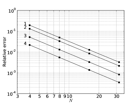
Figure 5.2. The relative error of the action versus the number of lattice sites per side $N$, for the actions 1, 2, 3, 4 described in section 5. The squares are the simulation data points and the solid lines are the second order polynomial fits. Errors are proportional to $h^{2}$ in all cases.

We plotted the absolute value of the relative deviation of the numerical action from the continuum action, as a function of the number of lattice sites per dimension. In all cases, the errors approach zero as the lattice resolution grows, so the action converges towards the continuum result. Using least squares second order polynomial fit, we determined that the relative error depends in the following way on the lattice constant $h$,

$$\mbox{Relative error}\approx Ch^{2},$$

where $C$ is some constant depending on the choice of gauge field. This is in accordance with the estimate 4.44.

Quantum $SU(2)$ gauge theory Monte Carlo computer simulations using the SGT action will be published in a companion article [8].

6. Conclusions

We have proposed a general formulation of lattice gauge theory on simplicial lattices. For any simplicial lattice of arbitrary shape, this action can by used for lattice gauge theory simulations or study of the classical equations of motion. Traditionally, lattice QCD simulations within physics have used a homogeneous mesh. Mesh refinement is a well established concept within the subject of FEM. We feel that it is well worth the effort to invenstigate the possibility of mesh refinement within classical and quantum gauge theory. Quantum lattice gauge theory simulations are very computer intensive. Therefore mesh refinement could be beneficial in cases where it makes sense to focus more computational effort on some subset of the simulation domain.

We have shown the consistency of this SGT numerical approximation to the continuous action, in the sense of approximation theory. The lattice gauge theory formalism is of such a complexity, that it makes sense to complement this theoretical proof with numerical “evidence”. We have provided this for a few different cases of gauge fields, for which the action was shown to converge towards the continuum result as the grid fineness increased.

References

• [1] Snorre H. Christiansen and Tore G. Halvorsen. A gauge invariant discretization on simplicial grids of the Schrödinger eigenvalue problem in an electromagnetic field. E-print, UiO, 2009.
• [2] Snorre H. Christiansen and Tore G. Halvorsen. A simplicial gauge theory. ArXiv e-prints, June 2010.
• [3] Snorre H. Christiansen and Ragnar Winther. On Constraint Preservation in Numerical Simulations of Yang–Mills Equations. SIAM Journal on Scientific Computing, 28(1):75–101, 2006.
• [4] Snorre Harald Christiansen, Hans Z. Munthe-Kaas, and Brynjulf Owren. Topics in structure-preserving discretization. Acta Numerica, 20:1–119, 2011.
• [5] Philippe G. Ciarlet. The Finite Element Method for Elliptic Problems, volume 4 of Studies in mathematics and its applications. North-Holland Publishing Company, 1. edition, 1978.
• [6] Michael Creutz. Quarks, Gluons and Lattices. Cambridge, Uk: Univ. Pr. (Cambridge Monographs On Mathematical Physics), 1986.
• [7] Brian C. Hall. Lie Groups, Lie Algebras, and Representations, An Elementary Introduction. Springer, 2. edition, 2004.
• [8] Tore G. Halvorsen and Torquil M. Sørensen. Lattice gauge theory using the Simplicial Gauge Theory action. In preparation, 2011.
• [9] Ralf Hiptmair. Finite elements in computational electromagnetism. Acta Numerica, 11(-1):237–339, 2002.
• [10] Peter Monk. Finite Element Methods for Maxwell’s Equations. Oxford Science Publications, reprinted edition, 2006.
• [11] Hans Munthe-Kaas and Brynjulf Owren. Computations in a free Lie algebra. Philosophical Transactions of the Royal Society of London. Series A: Mathematical, Physical and Engineering Sciences, 357(1754):957–981, 1999.
• [12] Michael E. Peskin and Daniel V. Schroeder. An Introduction to quantum field theory. Reading, USA: Addison-Wesley, 1995.
• [13] Steven Weinberg. The Quantum theory of fields. Vol. 1: Foundations. Cambridge, UK: Univ. Pr., 1995.
• [14] Steven Weinberg. The quantum theory of fields. Vol. 2: Modern applications. Cambridge, UK: Univ. Pr., 1996.
• [15] Hassler Whitney. Geometric integration theory. Princeton University Press, Princeton, N. J., 1957.
• [16] Kenneth G. Wilson. Confinement of quarks. Phys. Rev. D, 10(8):2445–2459, Oct 1974.
• [17] Chen-Ning Yang and Robert L. Mills. Conservation of isotopic spin and isotopic gauge invariance. Phys. Rev., 96:191–195, 1954.