Photometric redshift requirements for lens galaxies in galaxy-galaxy lensing analyses

Abstract

Weak gravitational lensing is a valuable probe of galaxy formation and cosmology. Here we quantify the effects of using photometric redshifts (photo-$z$) in galaxy-galaxy lensing, for both sources and lenses, both for the immediate goal of using galaxies with photo-$z$ as lenses in the Sloan Digital Sky Survey (SDSS) and as a demonstration of methodology for large, upcoming weak lensing surveys that will by necessity be dominated by lens samples with photo-$z$. We calculate the bias in the lensing mass calibration as well as consequences for absolute magnitude (i.e., $k$-corrections) and stellar mass estimates, for a large sample of SDSS Data Release 8 (DR8) galaxies. The redshifts are obtained with the template based photo-$z$ code ZEBRA on the SDSS DR8 $ugriz$ photometry. We assemble and characterise the calibration samples ($\sim$9k spectroscopic redshifts from four surveys) to obtain photometric redshift errors and lensing biases corresponding to our full SDSS DR8 lens and source catalogues. Our tests of the calibration sample also highlight the impact of observing conditions in the imaging survey when the spectroscopic calibration covers a small fraction of its footprint; atypical imaging conditions in calibration fields can lead to incorrect conclusions regarding the photo-$z$ of the full survey.

For the SDSS DR8 catalogue, we find $\sigma_{\Delta z/(1+z)}=0.096$ and $0.113$ for the lens and source catalogues, with flux limits of $r=21$ and $r=21.8$, respectively. The photo-$z$ bias and scatter is a function of photo-$z$ and template types, which we exploit to apply photo-$z$ quality cuts. By using photo-$z$ rather than spectroscopy for lenses, dim blue galaxies and $L_{*}$ galaxies up to $z\sim 0.4$ can be used as lenses, thus expanding into unexplored areas of parameter space. We also explore the systematic uncertainty in the lensing signal calibration when using source photo-$z$, and both lens and source photo-$z$; given the size of existing training samples, we can constrain the lensing signal calibration (and therefore the normalization of the surface mass density) to within 2 and 4 per cent, respectively.

1 Introduction

The current $\Lambda$CDM cosmological model is dominated by the unknown dark components of the universe: dark matter and dark energy (e.g., Komatsu et al., 2011). Gravitational lensing, the deflection of light from distant source galaxies by intervening masses along the line-of-sight (e.g., Bartelmann & Schneider, 2001; Refregier, 2003), has emerged as an enormously powerful astrophysical and cosmological probe. It is not only sensitive to dark energy through both cosmological distance measures and large-scale structure growth (Albrecht et al., 2006), but is also sensitive to all forms of matter, including dark matter. Measurements of the statistical distortion of galaxy shapes (or weak gravitational lensing) due to mass along the line-of-sight have been used in numerous studies to constrain the cosmological model, the theory of gravity, and the connection between galaxies and dark matter (e.g., most recently, Mandelbaum et al., 2006; Fu et al., 2008; Reyes et al., 2010; Schrabback et al., 2010). As a result, many more surveys are planned for the next two decades with weak lensing as a major science driver: KIDS, DES, HSC, Pan-STARRS, LSST, Euclid, and WFIRST.

In order to fully access the information encoded in gravitational lensing, redshift information is essential, as the conversion from distortions (gravitational shear) to mass depends on the lens and source redshifts via the critical surface density, expressed as

$$\Sigma_{c}=\frac{c^{2}}{4\pi G}\frac{D_{S}}{(1+z_{L})^{2}D_{L}D_{LS}}$$ (1)

in comoving coordinates (in physical coordinates, the expression lacks the factor of $(1+z_{L})^{-2}$). Here, $D_{L}$ and $D_{S}$ are angular diameter distances to the lens and source, and $D_{LS}$ is the angular diameter distance between the lens and source. Spectroscopic redshifts provide the best accuracy in determining $\Sigma_{c}$, but obtaining them for large, statistical samples of both lenses and sources is prohibitively expensive in terms of observing time and instrumentation. As a result, upcoming surveys will rely heavily upon less accurate photometric redshifts (photo-$z$) derived from multi-band imaging. Since we require source samples at higher redshift, and as the data pushes into the region of dim galaxies with poor photometry, the photo-$z$ may worsen even more. Consequently, it is of immediate interest to quantify how limited redshift accuracy (due to the use of photometric redshifts) propagates into lensing results.

Galaxy-galaxy lensing has been used in the past to quantify the connection between lens galaxies or clusters and their dark matter (DM) halos, in particular the total (average) mass profile around galaxies on $>20$kpc scales and the DM halo occupation statistics (Hoekstra et al., 2005; Heymans et al., 2006; Mandelbaum et al., 2006); can constrain the dark matter power spectrum when used in combination with the galaxy 2-point correlation function (Yoo et al., 2006; Cacciato et al., 2009; Baldauf et al., 2010; Oguri & Takada, 2011); and can constrain the theory of gravity when combined with clustering and redshift-space distortions (Zhang et al., 2007; Reyes et al., 2010). This paper addresses the use of photometric redshifts for both sources and lenses in galaxy-galaxy lensing, in the context of the Sloan Digital Sky Survey Data Release 8 (Eisenstein et al., 2011, and references therein; SDSS DR8 hereafter). Previous galaxy-galaxy lensing studies with SDSS have been limited to lenses with spectroscopic redshifts (e.g., Sheldon et al., 2004; Mandelbaum et al., 2006) or photo-$z$ with atypically high accuracy, such as those for Brightest Cluster Galaxies (e.g., Sheldon et al., 2009). Galaxy-galaxy lensing studies with other surveys have typically either involved an unusually large number of passbands yielding exceptionally good photo-$z$ (e.g., Kleinheinrich et al., 2006; Leauthaud et al., 2011), or have had limited area coverage and therefore relatively poor statistics compared with the SDSS studies (e.g., Parker et al., 2007).

Additional work must be done to allow galaxy-galaxy lensing to achieve its full potential with large, upcoming imaging surveys, and to extend to lens galaxy samples that lack spectra in SDSS. Lens galaxy samples that lack spectra in SDSS tend to be smaller, dimmer galaxies, or galaxies at higher redshifts: it would be interesting to extend galaxy-galaxy lensing studies to their DM halo masses and environments, including mass and redshift dependence. While studies with other surveys have extended into these regimes, they have typically involved deep but very narrow space-based data with significant cosmic variance (Heymans et al., 2006; Leauthaud et al., 2011) or wider but still relatively noisy ground-based survey data (Hoekstra et al., 2005).

In order to address galaxy-galaxy lensing based on SDSS DR8 photo-$z$, we have calculated a new set of photometric redshifts for the full flux-limited galaxy sample with extinction-corrected model $r<21.8$. We applied the publicly available photo-$z$ code Zürich Extragalactic Bayesian Redshift Analyzer (ZEBRA, Feldmann et al. 2006) to the SDSS $ugriz$ photometry. In this work, we demonstrate the photo-$z$ accuracy by comparing against several spectroscopic samples. In the course of this process, we identify several concerns related to the observing conditions in the imaging survey in regions that overlap the calibration survey, which will be generally applicable to any upcoming survey.

We define the criterion for a “better” photo-$z$ as a photo-$z$ that gives minimal scatter in the distribution of $z_{\rm spec}-z_{\rm phot}$, and hence the lowest scatter in the biases of any redshift-derived quantities, such as the lensing signal or the absolute magnitude. Note that we do not aim for the lowest bias in photo-$z$, according to the philosophy that biases can be corrected with a representative calibration sample, but rather the lowest uncertainty in the bias. This criterion results in a low uncertainty in the actual science analysis. A brief comparison to other publicly available photo-$z$ catalogues is presented. Improvements in the characterisation of photo-$z$ for the photometric galaxies can provide a substantial boost in statistics for current studies of the large scale structure. In addition, working with the photo-$z$ to the survey limiting magnitude with SDSS photometry will provide an ideal test case for future large surveys that rely upon photo-$z$ for all lensing calculations (which are, necessarily, dominated by galaxies near the flux limit).

With the improved and extended SDSS photo-$z$’s, we consider the application to galaxy-galaxy lensing. Photo-$z$ for weak lensing source galaxies in SDSS was investigated by Mandelbaum et al. 2008. Here, we address some additional nuances in the procedures from that work to define a fair calibration sample and to use it to estimate the lensing calibration bias. We then extend that formalism to use photo-$z$ for lenses, thus increasing the possible sample of lens galaxies by a factor of $\sim 40$ over the flux-limited MAIN spectroscopic sample ($r<17.77$) and colour-selected LRGs (luminous red galaxies; $r<19.5$). With an eye to using photo-$z$ for galaxy-galaxy lensing, we then test how the bias and scatter in the photometric redshifts for the SDSS photometric galaxy sample affect various derived quantities (including the lensing signal calibration, and the estimated luminosities and stellar masses) by direct comparison to their spectroscopic redshift (spec-$z$) counterparts. While Kleinheinrich et al. (2005) identify the need for lens redshift information over simply using a lens redshift distribution, our work is the first detailed demonstration of how to calibrate the effect of the lens photo-$z$ errors on other lensing observables.

The outline of the paper is as follows: we describe the data and calibration subsets in Sec. 2, and test the imaging quality in the regions overlapping the calibration samples for consistency with the average survey quality in Sec. 3. This latter step is crucial for ensuring that measurements using the calibration set are representative of the full SDSS DR8 sample of interest. We justify our choice of photo-$z$ method in Sec. 4. The photometric redshift accuracy results (bias and scatter) are discussed in Sec. 5. From the photometry and the photo-$z$, we also derive estimated absolute luminosity and stellar mass, described in Sec. 6.1 and Sec. 6.2, respectively. Sec. 6 then describes the resulting biases of derived quantities for galaxy-galaxy lensing applications. The lensing signal calibration is discussed separately in Sec. 7, and conclusions are presented in Sec. 8. We use a flat concordance WMAP7 (Komatsu et al., 2011) cosmology ($\Omega_{m}=0.27$, $h=0.702$) to calculate luminosity distances $D_{L}$ and angular diameter distances $D_{A}$ from redshifts.

2 Data

Here we describe the data sets used for this investigation: the SDSS photometric catalogue and the spectroscopic calibration sets.

2.1 SDSS photometry

The Sloan Digital Sky Survey (SDSS, York et al. 2000) is a shallow, wide-field survey that imaged 14 555 deg² of the sky to $r\sim 22$, and followed up roughly two million of the detected objects spectroscopically (Eisenstein et al., 2001; Richards et al., 2002; Strauss et al., 2002). The five-band ($ugriz$) SDSS imaging (Fukugita et al., 1996; Smith et al., 2002) was carried out by drift-scanning the sky in photometric conditions (Hogg et al., 2001; Ivezić et al., 2004; Padmanabhan et al., 2008) using a specially-designed wide-field camera (Gunn et al., 1998). All of the data were processed by completely automated pipelines that detect and measure photometric properties of objects, and astrometrically calibrate the data (Lupton et al., 2001; Pier et al., 2003; Tucker et al., 2006). The original goals of SDSS were completed with its seventh data release (DR7, Abazajian et al., 2009).

Accurate galaxy colours are needed in order to compute reliable photo-$z$’s. We have chosen our SDSS galaxy sample, described below, from the most recent SDSS-III Data Release 8 (Eisenstein et al., 2011, DR8). The galaxy colours obtained are based on the model magnitudes MODELMAG (Stoughton et al., 2002). The 5-band fluxes are estimated using a single galaxy model (the better fit of exponential or de Vaucouleurs) based on $r$-band imaging, which is then convolved with the band-specific point-spread function (PSF) and allowed to vary only in its amplitude in order to estimate the flux in each band. This procedure leads to a consistent definition of the magnitudes across all bands, despite the different PSFs. This method is superior to PSF-matching because it does not require convolutions of the data (convolutions lead to correlated noise, making estimation of the flux uncertainties challenging). A correction for galactic extinction was imposed using the dust maps from Schlegel et al. (1998) and the extinction-to-reddening ratios from Stoughton et al. (2002); we only use regions with $r$-band extinction $A_{r}<0.2$. This extinction cut is standard for many extragalactic observations, but is also particularly important here since dust extinction affects the relative magnitudes of the different bands, and the magnitude corrections become less reliable for higher extinctions. The photometry was calibrated using ubercalibration procedure (Padmanabhan et al., 2008), to ensure consistent calibration across the entire survey (within $1$ per cent), which is also important for photo-$z$ uniformity. Minor corrections were applied to the $u$ and $z$ band to correct to AB magnitudes ($-0.04$ and $+0.02$, respectively) for calculating the photometric redshifts. We note that using a more recent estimate on the absolute calibration, $m_{\rm AB}-m_{\rm SDSS}=-0.036,0.012,0.010,0.028,0.040$ for the $ugriz$ bands, does not significantly modify our results.

Requirements on the overall data quality for a region to be used are that the ubercalibration procedure (Padmanabhan et al., 2008) must classify the data as photometric (CALIB_STATUS $=1$); the $r$-band PSF FWHM must be smaller than 1.8^′′; and various Photo flags must indicate no major problems with the object detection and PSF estimation. In the acceptable regions, a total of 8720 square degrees, additional cuts were imposed when selecting galaxies; see Appendix A for details. In regions with multiple observations, we first chose the observation with the best seeing, and then imposed the magnitude cut.

The photometric (lens) catalogue is a purely flux-limited catalogue of galaxies with photo-$z$ information (this work). The full SDSS photometric catalogue has $r<22$, but to avoid the galaxies with very noisy photometry near the flux limit (based on previous findings, e.g. Kleinheinrich et al. 2005, that accurate lens redshift information is more important than source redshift information), we require $r<21$ for our lens sample. Galaxy detection is also more stable under different observing conditions with this magnitude cut, as discussed in Sec. 3.2.2, resulting in a relatively uniform lens galaxy number density across the survey. There are 28 036 133 objects in the photometric lens catalogue of $r<21$ (decreased from 64 750 701 in the full $r<22$ catalogue).

The source catalogue, in contrast, goes to a depth of $r<21.8$ and contains additional information about the galaxy shapes (Reyes et al. 2011 in prep.). In order to derive galaxy shapes without significant systematic error, the source catalogue has further quality cuts in order to ensure that the galaxies are sufficiently resolved compared to the PSF. It is an update of the Mandelbaum et al. (2005) source catalogue, with several technical improvements and with additional area. As for the old catalogue, the galaxy shape measurements are obtained using the REGLENS pipeline, including PSF correction done via re-Gaussianization (Hirata & Seljak, 2003) and with cuts designed to avoid various shear calibration biases. These cuts include a requirement that the galaxy be well-resolved in both the $r$ and $i$ bands, since the lensing measurements use an average of the $r$ and $i$ band shapes. There are 43 378 516 objects in the source catalogue that satisfy the resolution requirement (photo-$z$ quality cuts will reduce this further by $\sim 10$ per cent, as described in Sec. 5.1).

2.2 Calibration data sets

Quantities derived from photo-$z$’s, such as absolute magnitudes and the lensing signal calibration, will be biased due to photo-$z$ error. We estimate these biases (and their uncertainty) by measuring them on a representative subset of the SDSS catalogue for which spectroscopic redshifts are available. This calibration set must satisfy the following criteria: (1) Target selection is based on apparent magnitude only, with no colour selection (the latter often is used in spectroscopic surveys to select objects of certain redshift ranges and/or types)—unless two samples with complementary colour selection can be combined to make an effectively flux-limited survey. (2) If targeted off of different photometry than the imaging survey, then the limiting apparent magnitude must be somewhat deeper than the photometric survey, because increased flux uncertainty at the limiting magnitude will randomly scatter objects below and above the magnitude threshold. (3) The spectroscopic sample should not have any redshift failure modes that have a strong preference for particular galaxy types (magnitude, colour, or redshift). Note that some of these criteria are not absolute, in the sense that the analysis we describe could be adapted for calibration data sets that do not satisfy them perfectly, but it would significantly complicate the analysis and result in greater systematic error.

There are a limited number of surveys with spectroscopic or spectro-photometric redshift determinations that meet these criteria. The rest of this section describes each survey that we use for this analysis, noting in particular their survey targeting strategy, our quality cut criteria, and the resulting number of calibration galaxies. Figure 1 shows the footprints of SDSS and calibration subsamples; Table 1 summarises the number of galaxies from each survey that have been matched to our SDSS catalogue. Further cuts are needed so that the calibration and full samples are representative of the same populations (Sec. 3); there is an additional photo-$z$ quality cut (Sec. 5.1). These counts are shown in Table 1 in bold. After the full set of cuts, the parent calibration sample has 9 631 sources and 8 592 lenses; the former constitutes a substantial increase over Mandelbaum et al. (2008), which used 2 838 galaxies from only two of the calibration samples described below. While we have not addressed the spectroscopic failure rate on the calibration bias estimates, Mandelbaum et al. (2008, Sec. 5.5) studied the implications of a $\sim 5$ per cent failure rate and found minimal difference on the calibration bias.

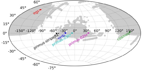
Figure 1: Footprints of the SDSS which satisfy our photometric quality criteria (8720 deg², shaded) and spectroscopic calibration subsamples (labeled). Each calibration subsample covers the full photometric depth of SDSS (except PRIMUS-stripe82, see text), but only covers $\sim 0.2$ per cent of the SDSS survey area.

	Redshift	Fraction	Counts
Survey	completeness	secure	lens	source
EGS	93	99	639	1060
			593	968
zCOSMOS	85	$>99.5$	775	1120
pCOSMOS	$>97$	97	2506	3644
COSMOS (union)			3281	4764
			2959	4293
VVDS	$55$	97	643	1132
			564	527
PRIMUS-02hr	$93$	$98$	(1436)	(2588)
…with DEEP2			1508	2908
			1357	1646
PRIMUS-23hr	$90$	$98$	(1612)	(3023)
…with DEEP2			1677	3307
			1547	1737
PRIMUS-stripe82	80	$98$	856	-
			786	-
Total			8592	9171

Table 1: A summary of the properties of our redshift calibration samples, including the redshift completeness (in per cent), the fraction of secure redshifts corresponding to that completeness (in per cent), and the original numbers of lens and source galaxies available in each one. The counts in bold are the actual number of objects used for calibration, after seeing (Sec. 3.2.3) and photo-$z$ quality cuts (Sec. 5.1) have been applied.

2.2.1 DEEP2 EGS

The DEEP2 Galaxy Redshift Survey (Davis et al., 2003; Madgwick et al., 2003; Coil et al., 2004; Davis et al., 2005, 2007) is a spectroscopic survey using the DEep Imaging Multi-Object Spectrograph (DEIMOS, Faber et al. 2003) on the Keck II Telescope at high spectral resolution ($R\sim 5000$). Of the four DEEP2 fields, we use spec-$z$’s from the Extended Groth Strip (EGS) field at RA$\sim$14hr, in which the targets include galaxies of all colours with $R_{AB}<24.1$. For $R>21.5$, the target selection deviates slightly from a purely flux-limited sample. As a result, a small fraction ($\sim 2$ per cent) of the SDSS-matched targets have been down-weighted based on colour; faint objects with $21.5<R_{AB}<24.1$ and colours suggesting a redshift $z<0.75$ receive lower targeting priority. However, this down-weighting was found to have minimal impact on the derived scatter and biases for the overall matched sample. Due to saturation issues, no objects brighter than $R_{AB}=17.6$ were targeted; these missing bright objects constitute a small fraction ($\lesssim 3$ per cent) of both our lens and source samples. There is a known redshift incompleteness which we discuss later in Sec. 3.4.

DEEP2 provides redshift quality flags, of which we keep flags 3 and 4, which correspond to 95 and $>$99.5 per cent repeatability, respectively. The good-quality ($q=3,4$) redshifts constitute $\sim 85$ per cent of the SDSS-matched calibration set, and the fraction are similar for both the lens and source sample. Over half of the remaining objects have their redshifts confirmed by visual inspection, such that the SDSS-matched EGS sample is 99 per cent secure, with 92 per cent completeness for both the lens and source samples (Table 1). Of the DEEP2 EGS spectroscopic galaxies, 639 and 1060 objects matched to the SDSS photometric catalogue ($r<21$) and source catalogue ($r<21.8$ with resolution cuts), respectively. The latter number differs from that in Mandelbaum et al. (2008) because of the use of a new reduction of the SDSS data to create a new source catalogue (see section 2.1).

2.2.2 zCOSMOS

The zCOSMOS-bright survey (Lilly et al., 2007, 2009) is a magnitude-limited spectroscopic survey on the Cosmological Evolution Survey (COSMOS) field (Capak et al., 2007; Scoville et al., 2007a, b; Taniguchi et al., 2007) with the VIsible Multi-Object Spectrograph (VIMOS, LeFevre et al. 2003) on the 8m European Southern Observatory Very Large Telescope (ESO VLT) at intermediate spectral resolution ($R\sim 600$). The selection is purely flux-limited at $15.0<I_{AB}<22.5$. We choose objects with confidence class 3 and 4; additionally, we include confidence class 9.5 objects, which have redshifts determined from a single emission line and which are consistent with the (30-band COSMOS) photometric redshifts discussed in section 2.2.3; these constitute $\sim$1 per cent of the SDSS-matched sample. The photo-$z$ agreement is necessary to break the degeneracy between H$\alpha$ and [OII]3727, when the doublet appears as a single line due to line broadening. Table 1 lists the number of objects from this survey available for photo-$z$ calibration.

Our matched zCOSMOS calibration sample is smaller than that from Mandelbaum et al. (2008) because $\sim 1/3$ of the SDSS imaging in the COSMOS region is classified as non-photometric (Mandelbaum et al., 2010), resulting in abnormally poor photo-$z$. Since the non-photometric regions are not representative of our source catalogue (for which we impose a photometricity cut), we eliminate the region of COSMOS for which the SDSS data are not photometric from consideration in this analysis, leaving 775 and 1120 lens and source galaxies (before further cuts that will be described below). An additional consideration regarding the COSMOS calibration sample is that the sky noise level in the SDSS imaging in the COSMOS region is significantly higher than what is typical for the SDSS survey overall. As we will show in Sec. 3.2, the consequence is an atypical deficit of fainter galaxies in the COSMOS calibration sample; we discuss how this deficit is handled in Sec. 7.2.

2.2.3 COSMOS photometric redshifts (pCOSMOS)

The first new calibration sample used in this work is the sample of flux-limited non-zCOSMOS galaxies in the COSMOS region, with photometric redshifts (Ilbert et al., 2009, pCOSMOS hereafter). Given the flux limit of the SDSS catalogue with respect to the COSMOS observations, and the accuracy demanded in the applications described in this paper, these COSMOS photo-$z$ are effectively the same as spectroscopic redshifts.

The pCOSMOS photo-$z$ are obtained from a $\chi^{2}$ template-fitting method, Le Phare. Highly accurate photo-$z$ result from the use of deep photometry in 30 bands (primary bands are $u^{*}$, $B_{J}$, $V_{J}$, $g^{+}$, $r^{+}$, $i^{+}$, $z^{+}$, and $K$), observed at various telescopes, primarily from Subaru and the Canada-France-Hawaii Telescope (CFHT). Comparing the COSMOS photo-z with the matching zCOSMOS redshifts, we estimate the scatter in the pCOSMOS calibration subset to be $\sigma_{\Delta z/(1+z)}\sim 0.009$, with an outlier rate of $\sim 1.2$ per cent for both the lens and the source samples (we find the bias to be negligible). COSMOS galaxies that have a zCOSMOS spectroscopic redshift have been removed, so that the zCOSMOS and pCOSMOS catalogues are disjoint (though they trace similar large-scale structures). There are 2506 and 3644 pCOSMOS matches to the photometric lens and source catalogues, respectively.

2.2.4 VVDS

The next new calibration sample is the VIMOS VLT Deep Survey (Le Fèvre et al., 2005, VVDS), another spectroscopic survey using the VIMOS instrument on the ESO-VLT. We use the public spectroscopic catalogue in the VVDS-F22 field, part of the VVDS-wide survey. This survey uses a lower resolution ($R\sim 230$ versus $600$) but similar exposure time ($3000$ versus $3600$ sec) compared to the zCOSMOS-bright survey. The VVDS-wide target selection is purely magnitude-limited ($17.5<I_{AB}<22.5$) with no colour selection. We select those galaxies with spectroscopic quality flags 3 and 4, with $\sim$96 and $\sim$99 per cent reliability, respectively. When combined, these constitute only $\sim$55 per cent of the SDSS-matched sample, suggesting a relatively low redshift success rate for this sample. Additionally, galaxies with qualities 13, 14 (broad emission line) or 23, 24 (serendipitous observations) are included; however these constitute a small fraction (3 per cent) of the SDSS-matched sample. In total, we use 643 lens and 1132 source galaxies with VVDS spectroscopic redshifts for SDSS photo-$z$ calibration, see Table 1. Because of concerns about the high spectroscopic redshift failure rate, we have (1) checked the colour and magnitude distributions of the VVDS-matched sample (Section 3.1) and (2) done all of the calculations of biases due to photo-$z$ error separately for individual spectroscopic subsamples. We find (Section 7.2) no systematic tendency for the VVDS results to differ with any of the others, suggesting that the redshift failure rate has not excessively biased the calibration sample properties.

2.2.5 PRIMUS

The final additions to our calibration sample come from the PRIsm MUlti-object Survey (PRIMUS; Coil et al., 2010, Cool et al. 2011 in prep.), a newly-completed survey that obtained spectro-photometric redshifts for $\sim 120~{}000$ galaxies to $i=23$ over an area of 9.1 deg². On the Inamori Magellan Areal Camera and Spectrograph (IMACS) on the Magellan I Telescope, PRIMUS uses a low-dispersion prism with $R\sim 40$ to efficiently survey wide areas and achieve a redshift accuracy of $\sigma_{z/(1+z)}\lesssim 0.005$ out to $z=1.2$. From the PRIMUS low-resolution spectra, the general shape of the spectrum, in addition to emission or absorption lines, is used to infer the redshift (Cool et al. 2011 in prep.). PRIMUS is generally a flux-limited survey (no colour selection); however there are a few relevant exceptions to this rule that we will discuss shortly. The target selection in most target fields used full and sparse sampling for $i<22.5$ and $22.5<i<23.5$, respectively, although the limiting magnitudes and reference band for these categories vary depending on the target field.

We included data from 3 fields, which we will denote PRIMUS-02hr, PRIMUS-23hr, and PRIMUS-stripe82. The PRIMUS-02hr and 23hr fields overlap the DEEP2 02hr and 23hr spectroscopic survey fields (these DEEP2 fields are $BRI$ colour-selected to include almost exclusively $z>0.7$ galaxies). The magnitude limits in these fields for full and sparse sampling were $R<22.8$ and $22.8<R<23.5$, respectively. The primary targeting strategy in these PRIMUS fields was to target the complement of the DEEP2 spectroscopic survey; hence the union of the PRIMUS and DEEP2 surveys in the 02hr and 23hr fields is essentially a flux-limited sample (Coil et al., 2010). We have verified that the relative weighting of DEEP2 to PRIMUS, which accounts for the targeting efficiency and survey area differences, is very near unity in the SDSS-matched sample in both fields. A fraction of the PRIMUS targets also have high-quality redshifts in DEEP2; for these, the spectroscopic redshifts from DEEP2 were used. The supplements from the DEEP2 survey with quality flag $>=3$ constitute $\sim$5 and $\sim$10 per cent of photometric lens ($r<21$) and source ($r<21.8$) catalogues, respectively. We limit our PRIMUS redshifts to those having quality flag of 3 or 4. The corresponding reliabilities are estimated at 93 and 97 per cent, respectively.

Like the other two fields, the PRIMUS-stripe82 calibration field overlaps the SDSS stripe-82 region, but in this case the PRIMUS targeting was carried out from single-epoch SDSS imaging to $r<22$ or $i<21$ with no colour selection. The fact that this targeting was carried out using a different (earlier) reduction of the SDSS imaging, in one particular observing run, results in targeting incompleteness at the faint end, with respect to the DR8 photometry. This issue, which is caused by the scatter in the derived magnitudes between different reductions, is apparent in Figure 2 below. Due to this incompleteness, which results in this region being quite different from the others with respect to the abundance of $r>21$ galaxies, we have opted to drop the $\sim$1k objects for the dimmer (source) catalogue. The matches to the brighter lens catalogue were used for our calibration; these include $856$ objects (80 per cent completeness). The combination of the three PRIMUS fields adds over 3000 lens and 5000 source calibration galaxies to our calibration sample.

Table 1 shows a summary of the number of galaxies passing the cuts from each of the above calibration fields, and the remaining fraction after cuts described below (Sec. 3.2.3, Sec. 5.1) are applied.

3 Calibration set adjustments

The spectroscopic calibration sample is an extremely small subset of the SDSS photometric sample (Fig. 1). To ensure that conclusions derived from these calibration samples are applicable to the full SDSS sample, the following differences between calibration subsamples must be addressed:

• The differing spectroscopic survey completeness in each subsample.

• The differing SDSS observational conditions in the imaging data overlapping each spectroscopic calibration subsample (SDSS completeness).

• The specific large-scale structure (LSS) in each of the calibration fields (sample variance).

We generate two calibration sets, one each for the lens and source catalogue. The first two issues are most relevant for the source catalogue, as its faint galaxies are less robust to these issues.

3.1 Spectroscopic completeness

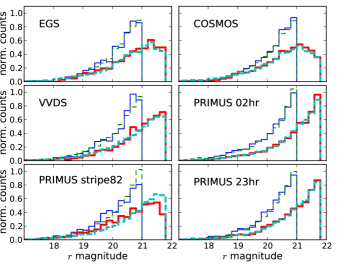
Figure 2: The $r$-band magnitude distribution of the spectroscopic calibration samples, matched to the source ($r<21.8$, thick solid line) and photometric ($r<21$, thin solid line) SDSS catalogues, respectively. The corresponding dashed lines indicate the underlying SDSS distribution in the same area. There is a noticeable discrepancy within $\sim 0.5$ mag of the limiting magnitude for the PRIMUS-stripe82 spectroscopic set relative to SDSS, indicating spectroscopic incompleteness for the source sample at $r>21$ (see text).

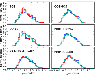
Figure 3: The $g-r$ colour distribution of the spectroscopic calibration samples, matched to the source ($r<21.8$, thick solid line) and photometric ($r<21$, thin solid line) SDSS catalogues, respectively. The corresponding dotted lines are the underlying SDSS distribution in the same area. Difference in the dotted and solid lines indicates colour dependence of the success rate of the spectroscopic redshifts. VVDS shows some colour dependence ($g-r$) of the redshift success rate (see text).

The SDSS-matched spectroscopic calibration samples described in Sec. 2.2 have varying degrees of magnitude and colour completeness. Here we address the targeting incompleteness of the spectroscopic set with respect to the SDSS sample. The completeness of the SDSS imaging data itself is addressed in Sec. 3.2.

Figure 2 shows the $r$-band magnitude distribution of the spectroscopic sample, matched to the source ($r<21.8$) and photometric ($r<21$) SDSS catalogues (the thick and thin solid lines, respectively). The corresponding dashed lines show the underlying SDSS distribution in the same area. The PRIMUS-stripe82 field shows a noticeable discrepancy in the number counts at $r>21$ between the spectroscopic redshift sample and the underlying magnitude distribution. The magnitudes used for target selection in this field came from an earlier photometric reduction of the SDSS single-epoch imaging. The earlier reduction resulted in magnitude incompleteness at the faint end, caused by the scatter in the derived magnitudes between different reductions. Since the PRIMUS-stripe82 source-matched catalogue also shows a lack of high redshift ($z>0.7$) objects which are important for source catalogue calibration, we remove this field from the source calibration set (but not from the lens calibration set, since there are fewer discrepancies there).

Similarly, the thick and thin solid lines in Figure 3 show the $g-r$ colour distribution of the spectroscopic sample. Differences in the dashed (underlying SDSS distribution) and solid (distribution of the high-quality spectroscopic redshifts) lines indicate colour dependence of the spectroscopic redshift success rate. Most samples show no noticeable discrepancy in the $g-r$ colour distributions. We have examined all 4 colours ($u-g$, $g-r$, $r-i$, $i-z$), and found VVDS shows some discrepancy in the $g-r$ colour (shown), and to a lesser degree, in $r-i$. Although this is alarming, we have otherwise not found anomalous behaviour in the VVDS subsample; the redshift distribution, the photo-$z$ spectral template type distribution, and the various derived biases are consistent with those for the other subsamples. Hence we keep the VVDS calibration field. We note that the PRIMUS-stripe82 source-matched sample shows discrepancy in the $r-i$ and $i-z$ colours, but in such a way that mimics the colour distribution of the brighter sample; this indicates consistency with the incompleteness in the $r$ magnitude distribution.

3.2 SDSS completeness

Here we address completeness of the SDSS itself. Different SDSS fields exhibit different $r$ magnitude distributions, due to the varying observational conditions. This can be seen in the different panels of Fig. 2, which have different dashed histograms (which are for the source samples in these regions before requiring a match in the spectroscopic data), though in the absence of other information we cannot rule out that these variations are due to sampling variance rather than observing conditions. Here we will demonstrate how the non-uniform seeing and sky noise over the photometric survey area, which affects the depth to which an object can be detected, can give rise to the differences in this figure. For the calibration set to fairly represent the SDSS as a whole, we need to understand how the observing conditions in each field differ from the median of the whole survey, and correct for any severe deviations from typical conditions.

3.2.1 SDSS observing conditions

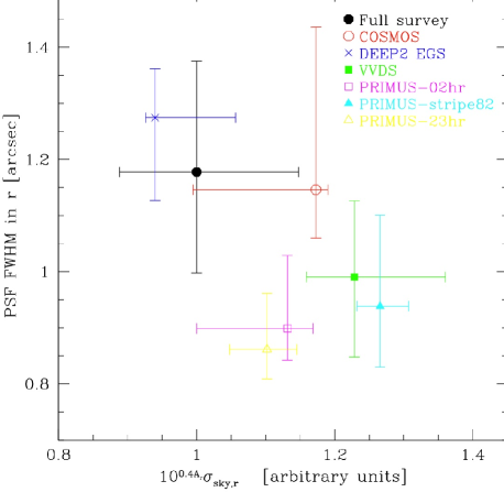
Figure 4: SDSS $r$-band observation conditions (sky noise, as described in the text, and seeing) for each of the calibration fields and the SDSS full survey.

Figure 4 shows the SDSS observation conditions in $r$-band, for the source galaxies in each of the calibration fields and in the full SDSS survey. Here we have used galaxies that are well-resolved to trace the observing conditions, which means that we will be skewed towards better observing conditions (as compared to if we had done the calculation using pure areas). This methodology explains why the seeing is noticeably better than the typical value that is commonly used for SDSS, 1.4^′′. Points indicate a median value, and error bars indicate the 68th percentile. To calculate sky noise (horizontal axis), we approximate the Poisson noise due to the sky and dark current as

$$\sigma_{\text{sky}}(\text{counts})=\sqrt{\frac{\text{sky}}{\text{gain}}+\text{dark current}}.$$ (2)

This is a reasonable approximation for galaxies with $r\gtrsim 20$, where the Poisson noise due to the galaxy flux itself is negligible. We then convert this to the sky noise in nanomaggies using the calibration from ubercal (Padmanabhan et al., 2008); this noise in nanomaggies determines the $S/N$ for a galaxy with a given size and flux, at fixed seeing and galactic extinction $A_{r}$. Then, we multiply the sky noise estimates by $10^{0.4A_{r}}$; in reality, of course, extinction modulates the flux, but this has the same effect on the S/N as increasing the sky noise by this factor. Finally, we have divided out by the median value of $10^{0.4A_{r}}\sigma_{\text{sky}}$ for the survey. When the sky noise is large, more galaxies at a given flux will fail the $S/N>5$ object detection filter; this is also true for worse seeing, since that filter is imposed within a PSF rather than using the entire galaxy flux.

The $r$-band PSF FWHM in arcsec is shown on the vertical axis. In poor seeing, the observed magnitudes are noisier (because the galaxy is spread out over more pixels and has greater sky noise contribution), and star-galaxy separation is more challenging (more galaxies get classified as stars).

As shown, the observing conditions in the calibration fields are not typical of the full SDSS DR8 sample. The EGS is within the $1\sigma$ range of observing conditions for both seeing and sky noise. The COSMOS data have relatively high sky noise for more than half the area, which will lead to reductions in galaxy $S/N$ of $\sim 20$ per cent compared to that for similar galaxies in the EGS. PRIMUS-02hr and PRIMUS-23hr are marginally within the typical region for sky noise, and VVDS and PRIMUS-stripe82 are at higher sky noise; but all four fields have significantly better seeing than that of the full SDSS. The reason for this trend is that all of these samples are on stripe 82, which has many observations. Since we select towards observations with better seeing (preferable for lensing) when creating the source catalogue, we get atypically good seeing. The fact that the extinction is on the higher end for these regions increases the effective sky noise, though it is not the only (or even the main) reason why these calibration samples have higher sky noise than is typical. As we will see in the next section, to lowest order we expect that the changes in sample properties due to having atypically good seeing will oppose (and even outweigh) the changes in sample properties due to atypically high sky noise for these stripe 82 samples.

3.2.2 Effect on number counts

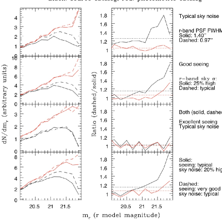
Figure 5: An illustration of how observing conditions can modulate the observed galaxy number densities, based on comparisons of pairs of runs with identical area coverage but different observing conditions in stripe 82. Each row utilizes a different pair of runs with conditions given on the right. Black lines are for the source catalogue, red lines are for the full photometric catalogue (no lensing selection). Left column: Histogram of $r$-band model magnitudes, with the different colours indicating which catalogue was used, and different line types indicating the observing conditions as labeled on the right-hand side. Right column: Solid lines show the ratio of the histograms with different observing conditions from the left column, always putting the dashed histogram in the numerator. The dotted lines show the ratio of the total number of galaxies in the region as defined using the full sample (averaged over magnitudes).

In Fig. 5, we illustrate the effect of observing conditions on the overall counts and magnitude distribution of galaxies, which is helpful in understanding the behaviour of the galaxy counts in the different calibration samples. We make this comparison by selecting pairs of runs overlapping the PRIMUS-02hr and PRIMUS-23hr regions, with different observing conditions but exactly the same area coverage. Thus, any differences in the galaxy apparent magnitude distributions in the pairs of runs are due to the observing conditions, rather than intrinsic differences in the galaxy populations. The four rows correspond to four different scenarios, with r model magnitudes on the horizontal axis and number counts on the vertical axis. At left are the counts (for both fields, source and photometric lens catalogues). At right the ratio between counts for the runs with two different observing conditions is shown. In the top row, results are given for nearly identical (within 10 per cent) sky noise, but 45 per cent difference in the seeing. (This is done by comparing runs that are $\sim 20$ per cent better and worse than the survey median seeing.) The second row corresponds to seeing that is nearly identical (within 10 per cent) and a bit better than the survey median, but sky noise that differs by 30 per cent. The third row shows nearly identical conditions for the seeing and sky noise, to illustrate the magnitude of the differences that can occur just due to Poisson noise. The fourth row shows the case of two effects going in the same direction: 25 per cent difference in seeing and 15 per cent difference in sky noise, where one run is better in both cases (better seeing and lower sky noise).

For the photometric catalogue, the effect of seeing on the galaxy number counts is small ($<5$ per cent, as shown in the top row) and nearly constant over all magnitudes. This change in counts may be due predominantly to the star-galaxy selection. For the source catalogue, which has apparent size selection, the effect of seeing is larger (as we would expect), and varies more strongly with magnitude, from a nearly constant 20 per cent below $r<21$ to typically 50 per cent above $r>21$.

The signature of sky noise, shown in the second row, is somewhat different. It preferentially reduces the number counts at fainter magnitudes for the purely flux-limited galaxy sample. The overall effect of 5 per cent is actually dominated by the fainter parts of the catalogue, with almost no effect below $r<21.4$ and a gradually increasing effect at fainter magnitudes, up to 35 per cent. In contrast, for the source catalogue, the average difference is more significant (15 per cent) and becomes noticeable at brighter magnitudes, from $r>\sim 20.8$. The third row shows that for identical observing conditions, the samples that are selected in both the photometric and source catalogue are statistically identical, with $<5$ per cent fluctuations in the magnitude histograms. Examination of the actual galaxy samples indicates significant noise, with fainter galaxies being scattered in and out of the sample, such that the fraction of galaxies in both catalogues is $\sim 70$ per cent. Finally, the fourth row is not at all surprising considering the first and second: we see both the effects of seeing and of sky noise.

From this analysis we see that the flux-limited photometric lens sample, with $r<21$, is not strongly affected by the changes in observing conditions, because these effects are only very significant ($>5$ per cent) in objects fainter than $r\sim 21.4$. In contrast, the source number density is strongly affected by observing conditions. We now turn to the corrections we make to account for these effects in our calibration samples, to make them more representative of the full SDSS area.

3.2.3 Corrections for observation conditions

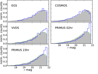
Figure 6: The $r$-band magnitude distribution of the source catalogues for each spectroscopic subsample (line histograms), in contrast to the SDSS distribution (grey block histograms). The differing SDSS observing conditions cause variable magnitude completeness near the limiting magnitude $r\sim 21.8$. We adjust the galaxy population in VVDS, PRIMUS-02hr, and PRIMUS-23hr fields to match the SDSS completeness by systematically trimming the lowest resolution objects (dotted lines), such that the resulting $r$ magnitude distribution matches that of SDSS (see text).

Figure 6 explicitly compares the magnitude distribution for each of the source calibration samples to that of the whole of SDSS. Objects in the fields that overlap SDSS stripe 82 (VVDS, PRIMUS-02hr and PRIMUS-23hr) tend to have high completeness near the limiting magnitude; this is because there are many repeat observations in this stripe, and the source catalogue reductions choose the observation of each galaxy that has the best seeing.

Since stripe 82 only covers a small fraction of the SDSS footprint ($\sim$3 per cent) and is not representative of the whole of SDSS, we would like to correct for the excess faint objects. These objects are removed as follows: (1) we bin the galaxies by their $r$ magnitudes, and (2) for each magnitude bin, we remove the lowest apparent resolution galaxies until the resulting magnitude histogram matches that from all of SDSS. This process removes $\sim 40$ per cent of the objects in a given field. (Figs. 2 and 3 do not include this cut.)

The COSMOS field has poor sky noise, and in general has unusually bad observational conditions compared to the rest of SDSS (e.g., a third of the COSMOS field is not classified as photometric in SDSS, so we have eliminated that portion of the field). This leads to a deficit of faint galaxy detections; however, we cannot artificially add objects that are missing from the catalogues. Hence, when using the COSMOS source calibration set, we have applied empirical corrections to the derived values (see Sec. 7.2).

3.3 Sample variance

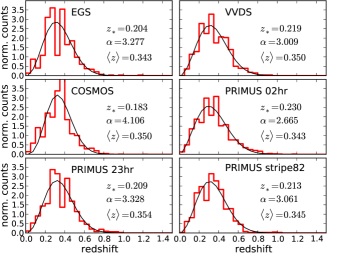
Figure 7: The observed redshift distributions of the lens calibration subsamples are shown as thick line histograms. The fits to the underlying redshift distribution (thin lines), along with the best-fitting parameters, are also shown.

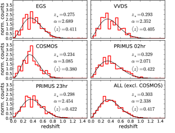
Figure 8: Analogous to Fig. 7, except these are for the source calibration subsamples, along with the combination of all the source calibration subsamples excluding the COSMOS field (see text).

Table 2: Fitting parameters for redshift distributions of the subsamples. The source samples for VVDS, PRIMUS 02hr and PRIMUS 23hr have the seeing cuts (Sec. 3.2.3) applied; the redshift distribution parameters before and after photo-$z$ cuts (Sec. 5.1) are listed.

Sample	$N_{\rm gal}$	$z^{*}$	$\alpha$	$\langle z\rangle$
Photometric (lens) sample with r$<$21
EGS	639	0.209	3.050	0.336
VVDS	643	0.224	2.710	0.338
COSMOS	3281	0.207	3.139	0.339
PRIMUS 02hr	1508	0.243	2.325	0.334
PRIMUS 23hr	1677	0.220	2.987	0.349
PRIMUS stripe82	856	0.223	2.718	0.336
Photometric (lens) sample with r$<$21 and photo-$z$ quality cuts
EGS	593	0.204	3.277	0.343
VVDS	564	0.219	3.009	0.350
COSMOS	2959	0.183	4.106	0.350
PRIMUS 02hr	1357	0.230	2.665	0.343
PRIMUS 23hr	1547	0.209	3.328	0.354
PRIMUS stripe82	786	0.213	3.061	0.345
Source sample with r$<$21.8 (includes seeing cuts)
EGS	1060	0.289	2.399	0.404
VVDS	609	0.253	2.101	0.391
COSMOS	4764	0.253	2.560	0.368
PRIMUS 02hr	1834	0.344	1.854	0.411
PRIMUS 23hr	1896	0.308	2.257	0.416
Source sample with r$<$21.8 and photo-$z$ quality cuts
EGS	968	0.275	2.689	0.411
VVDS	527	0.293	2.352	0.405
COSMOS	4293	0.234	3.085	0.380
PRIMUS 02hr	1646	0.329	2.071	0.422
PRIMUS 23hr	1737	0.298	2.454	0.422

Each individual field has distinct large-scale structure due to galaxy clustering. Thus, the observed $\mathrm{d}N/\mathrm{d}z$ in each field differs from the true underlying redshift distribution $\mathrm{d}N/\mathrm{d}z$, which is unknown but is expected to be smooth. We model this smooth distribution by fitting to a functional form (our bias analysis does not depend significantly on the detailed form of the curve, as discussed in Mandelbaum et al. 2008)

$$\frac{\mathrm{d}N}{\mathrm{d}z}\propto\left(\frac{z}{z_{*}}\right)^{\alpha-1}\exp\left[-\frac{1}{2}\left(\frac{z}{z_{*}}\right)^{2}\right]$$ (3)

which has a mean redshift of

$$\langle z\rangle=\frac{\sqrt{2}\;z_{*}\;\Gamma[(\alpha+1)/2]}{\Gamma[\alpha/2]}.$$ (4)

Figures 7 and 8 show the true redshift distributions for each of the lens and source calibration samples, along with their fitted curves and parameters. Following Sec. 4.2 of Mandelbaum et al. (2008), the histograms are $\chi^{2}$-fit to Eq. (3) with flat weights while constraining the area under the curve to equal to the galaxy count $N_{\rm gal}$; the redshift histograms of binning width $\Delta z=0.05$ were bootstrap resampled to obtain LSS error estimates to the fitting curve. The distributions shown here were derived after imposing cuts to correct for different seeing in the calibration samples on stripe 82, as discussed in Sec. 3.2.3. When further photo-$z$ quality cuts are applied (Sec. 5.1), the distribution shifts somewhat; the fit parameter values for both cases are listed for each catalog and subsample in Table 2.

The errors in the fits to the redshift distribution for each sample come primarily from sampling variance; thus, when fitting to the overall calibration sample redshift distribution, these fluctuations are reduced (more significantly than one would expect fluctuations due to Poisson noise to be reduced). The significant smoothing out of LSS can be seen in the bottom right panel of Fig. 8, where we plot the sum of all source subsamples, excluding the COSMOS region (this region was excluded due to its difference in sky noise which should result in a different intrinsic redshift distribution). This curve is our best estimate for the source catalogue redshift distribution; a similar smoothing in LSS is seen for the lens sample, for the sum of all 6 subsamples. These figures show that the upper limit in redshifts is around $z\sim 0.8$ ($z\sim 1.0$) for the lens (source) catalogues, with a mean redshift of $0.34$ ($0.41$). We note that the parameters $z_{*}$ and $\alpha$ are degenerate to some extent (small $\alpha$ brings the peak to higher redshifts, while high $z_{*}$ spreads out the overall distribution), and hence there is considerably more uncertainty in the parameters in $[z_{*},\alpha]$ than in the mean redshift $\langle z\rangle$. The fit parameter errors can be estimated by modulating the redshift bin counts to simulate LSS (Mandelbaum et al., 2008), or by looking at the variation in the fit values of the different subsamples.

3.4 Other incompleteness

The EGS matched samples have a deficiency of $z\sim 0.3$ galaxies, which is due to instrumental limitations of the survey (Newman et al. 2011 in prep., priv. comm.). Such a deficiency cannot easily be remedied; however, we find that, at this redshift, this deficiency does not affect the derived lensing signal calibrations when using source photo-$z$, which is more sensitive to the distribution of high-redshift ($z>0.6$) objects. However, this does affect the calibration for lens photo-$z$, and care must be taken when the EGS lens calibration subset is used on its own (Sec. 7.3).

4 Photo-$z$ Method

We chose the template-based ZEBRA code (Feldmann et al., 2006) to estimate our photo-$z$’s based upon the SDSS $ugriz$ bands. There are several public SDSS photo-$z$ catalogues for the full photometric sample, all of which are based on training-set methods: two by Oyaizu et al. (2008), available in the DR8 CAS database, one by Budavári et al. (2000) in SDSS DR7 (Abazajian et al., 2009) CAS database, and another by Cunha et al. (2009).

These photo-$z$ methods were included among those tested in Mandelbaum et al. (2008), for source galaxy redshifts. However, as those estimates were based on earlier Data Releases (5 and 6), including more preliminary photo-$z$ estimation procedures and photometry that lacked ubercalibration, the results of the tests in Mandelbaum et al. (2008) do not necessary apply to these new DR7 and DR8 versions. In Appendix B, we compare the photo-$z$’s in those publicly available SDSS DR8 catalogue, and give our reasons for choosing to use ZEBRA, another template-based method that will be described below.

Template-fitting photo-$z$ algorithms operate, broadly speaking, as follows: Given a set of spectral energy distribution (SED) templates, the SEDs are projected onto passbands shifted on a grid of redshifts, from which the predicted photometry, and hence colour, for each case (template type and redshift) is calculated. The observed colours are then compared against the model magnitudes, with a $\chi^{2}$-minimisation over all bands used to determine the best-fit redshift and spectral type. The choice of templates is crucial for obtaining quality photo-$z$, so we will begin by describing our choice of templates.

4.1 Templates

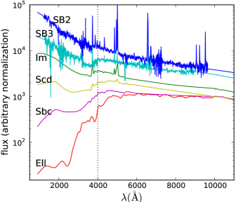
Figure 9: The six SED templates used in the ZEBRA photometric redshifts. Four templates (labeled Ell, Sbc, Scd and Im) are observed spectra from Coleman et al. (1980), and two (SB2 and SB3) are synthetic starburst spectra (Kinney et al., 1996). Five templates were interpolated between the existing 6 templates, for a total of 31 templates which were used for ZEBRA photo-$z$ estimation.

Templates can be obtained from observation, or generated from stellar population synthesis (SPS) models. We choose the set of six SED templates as described in Benítez (2000), and used in ZEBRA (Feldmann et al., 2006). They are shown in Figure 9. The set consists of four templates from Coleman et al. (1980, CWW hereafter), which are SEDs observed across a wavelength baseline of 1400Å $<\lambda<10000$Å in the local ($z\sim 0$) universe; they are supplemented by two synthetic blue spectra, using the GISSEL synthetic models (Bruzual & Charlot, 1993). While each of these templates have been linearly extrapolated into the UV and NIR wavelengths based on different synthetic models, these extensions are largely irrelevant to the optical filter set that we use (3000Å $<\lambda<10000$Å) for the redshift range relevant for our sample ($z<1.5$). The CWW templates have been widely employed and are known to generate reliable photometric redshift estimates, although training and tweaking the templates improves redshift estimates (Ilbert et al., 2006; Feldmann et al., 2006).

In particular, Ilbert et al. (2006) find that these templates work reasonably well for VVDS data, with a photo-$z$ scatter of $\sigma_{\Delta z/(1+z)}\sim 0.029$ given deep photometry covering a similar range of wavelength to ours ($u^{*}g^{\prime}r^{\prime}i^{\prime}z^{\prime}$ and $BVRI$, with additional $JK$ bands for 13 per cent of galaxies). With SDSS photometry, we expect a larger scatter because of the shallower photometry and lack of extra bands.

4.2 ZEBRA options

For the different template-fitting photo-$z$ codes, their photo-$z$ accuracy are very similar if the same set of templates is used, since most methods use essentially similar basic procedures of $\chi^{2}$ minimization (Hildebrandt et al., 2010). However, in addition to template choice, ZEBRA offers several options that enhances the photo-$z$ calculations. Priors on the redshift distribution or other conditions may be applied when calculating $\chi^{2}$. Additional features, such as iterative photometry self-calibration, template optimisation, $k$-correction tables, and different modes of photo-$z$ and template type determination, are also available. We detail our choices of such ZEBRA options here.

4.2.1 ZEBRA parameters

We ran ZEBRA in the maximum-likelihood (ML) mode. This was chosen over the Bayesian mode (BP), which allows for a Bayesian prior on the redshift distribution, per template type and redshift range. Although the latter method removes the photo-$z$ bias to some extent, we find that it significantly adds to the scatter in photo-$z$, which is the quantity of most concern for our application. Because the original CWW templates are known to generate photo-$z$’s with bias (Fig. 5 of Feldmann et al., 2006), applying a “correct” redshift distribution prior (the estimated redshift distribution of the given sample) will decrease the bias while increasing the scatter.

We use the following set of parameters to obtain our photo-$z$’s. The SED templates were interpolated with 5 new templates between each of the 6 given templates, resulting in a total of 31 templates. The redshifts are allowed to vary in steps of 0.0025 from 0 to 1.5, with no smoothing of the filter bands. We have applied a prior of photo-$z$ $<1.5$, which is reasonable for single-epoch SDSS photometry (most galaxies within our magnitude limit are at $z<1.0$). Similarly, we do not correct for the Lyman-$\alpha$ IGM absorption (Madau, 1995; Meiksin, 2006) since it is only relevant for objects at $z>3$.

4.2.2 ZEBRA self-calibration

In principle, the template-fitting may benefit from use of a spec-$z$ training set to calibrate the zero-point magnitude of the photometry; here, this procedure is unnecessary as we find no offset for SDSS. This is as expected given the excellent photometric calibration (Padmanabhan et al., 2008). The SED templates can be modified based on a spec-$z$ calibration set, but we also find this template modification procedure unnecessary. While template calibration have been shown to work with samples of better photometry (Ilbert et al., 2006; Feldmann et al., 2006), our attempts at template modification suggested that we were only fitting to the photometric noise, as an improvement to the templates and photo-$z$ error based on one calibration set did not translate to less scatter in the photo-$z$ computed with other calibration sets. Moreover, the modifications to the templates did not look remotely physical. The difference between our finding and the improvements found in Feldmann et al. (2006) most likely originates from the low signal-to-noise of our photometry.

4.3 $k$-correction

ZEBRA, as a template fitting method, allows estimates of absolute magnitudes and stellar masses. To obtain these, we have utilised the $k$-correction table (a list of theoretical magnitudes for each SED template at all redshifts; Eq. (7) below) generated by ZEBRA. This table is then modified according to the procedures below, to allow versatility in our $k$-corrections. Factors of $\log_{10}(1+z)$ that appear with different signs and/or prefactors in previous papers on the topic of $k$-correction are elucidated here.

$k$-correction encapsulates the magnitude corrections beyond the simple distance modulus, such that

$$M_{Q}=m_{R}-DM(z_{\rm gal})-K(z_{\rm gal},\;T,\;R,\;Q).$$ (5)

Here, $M_{Q}$ is the rest-frame absolute magnitude in filter $Q$, $m_{R}$ is the observed magnitude in band $R$, $DM(z_{\rm gal})=5\log_{10}(D_{L}/10{\rm pc})$ is the distance modulus (where $D_{L}=D_{L}(z_{\rm gal})$ is the luminosity distance in parsecs), and $K(z_{\rm gal},T,Q,R)$ is the $k$-correction factor. The $k$-correction depends on the galaxy redshift $z_{\rm gal}$, template type $T$, the band $R$ in which the magnitude is observed, and the desired band $Q$ for the absolute magnitude. To minimise the degree of $k$-correction in a sample, $Q$ is often chosen such that it is the $R$ band filter redshifted to the sample median redshift $z_{0}$: i.e., $Q=^{z_{0}}\!\!\!R$, or $Q(\lambda(1+z_{0})^{-1})=R(\lambda)$. Then $k$-corrections are calculated as (Hogg et al., 2002; Blanton & Roweis, 2007)

$$K(z_{\rm gal},\;T,\;R,\;Q) = 2.5\log_{10}(1+z_{\rm gal})$$

$$+\;\hat{m}(z_{\rm gal},\;T,\;R)-\hat{m}(z=0,\;T,\;Q)$$

where ZEBRA tabulates the AB magnitudes $\hat{m}$ for an array of redshifts $z_{\rm gal}$:

$$\hat{m}(z_{\rm gal},\;T,\;R)=-2.5\log_{10}\left[\frac{\int d\lambda\;\lambda\;F_{\lambda}^{T}[\lambda(1+z_{\rm gal})^{-1}]R(\lambda)}{\int d\lambda\;\lambda\;g_{\lambda}^{AB}(\lambda)R(\lambda)}\right].$$ (7)

Here the quantity in square brackets is the flux ratio that defines the AB magnitude. Since the observed SED output of a galaxy of type $T$ at redshift $z_{\rm gal}$ is

$$(1+z_{\rm gal})^{-1}F_{\lambda}^{T}[\lambda(1+z_{\rm gal})^{-1}]\,d\lambda$$ (8)

where $F_{\lambda}^{T}(\lambda)\,d\lambda$ is the rest-frame SED, we see that the $2.5\log_{10}(1+z_{\rm gal})$ factor which appears in the first term of Eq. (4.3) is from correction to the tabulated magnitude $\hat{m}(z_{\rm gal})$ for the loss in photon energy (flux) due to redshift. The reference SED relative to which AB magnitudes are defined is $g_{\lambda}^{AB}(\lambda)$, and $[\lambda\;g_{\lambda}^{AB}(\lambda)]\propto\lambda^{-1}$, since $g_{\lambda}^{AB}$ is proportional to $\lambda^{-2}$. The arbitrary normalisations in both $g^{AB}$ and $F_{\lambda}$ cancel out when we take the difference of $\hat{m}$.

If $Q$ is $R^{\prime}$ redshifted by $z_{0}$, such that $R^{\prime}$ is one of the existing bands (i.e., $Q(\lambda(1+z_{0})^{-1})=R^{\prime}(\lambda)$), then the tabulated values can also be used to obtain $\hat{m}(z=0,T,Q=^{z_{0}}~{}\!\!\!\!\!R^{\prime})$:

$$\hat{m}(0,\;T,\,^{z_{0}}\!R^{\prime}) \equiv -2.5\log_{10}\left[\frac{\int d\lambda\;\lambda\;F_{\lambda}^{T}(\lambda)Q(\lambda)}{\int d\lambda\;\lambda^{-1}\;Q(\lambda)}\right]$$ (9)

$$= -2.5\log_{10}\left[\frac{\int d\lambda^{\prime}\;\lambda^{\prime}\;F_{\lambda}^{T}[\lambda^{\prime}(1+z_{0})^{-1}]R^{\prime}(\lambda^{\prime})}{(1+z_{0})^{2}\int d\lambda^{\prime}\;\lambda^{\prime-1}R^{\prime}(\lambda^{\prime})}\right]$$

$$= \hat{m}(z_{0},\;T,\;R^{\prime})+5\log_{10}(1+z_{0})$$

where $\lambda^{\prime}\equiv\lambda(1+z_{0})$. The $k$-correction from the ZEBRA tabulated values are then

$$K(z_{\rm gal},\;T,\;R,\;^{z_{0}}\!R^{\prime}) = 2.5\log_{10}(1+z_{\rm gal})-5\log_{10}(1+z_{0})$$ (10)

$$+\;\hat{m}(z_{\rm gal},\;T,\;R)-\hat{m}(z_{0},\;T,\;R^{\prime})$$

where $R$ and $R^{\prime}$ can be any of the available filter bands. For the special case where $R=R^{\prime}$ and $z_{\rm gal}=z_{0}$, we have

$$K(z_{0},\;T,\;R,\;^{z_{0}}\!R)=-2.5\log_{10}(1+z_{0})$$ (11)

which does not depend on the template type $T$ by construction, but is non-zero. Since the SED type $T$ is uncertain in all photo-$z$’s, the observed band $R$ should be chosen such that it maximally overlaps with ${}^{z_{0}}\!R^{\prime}$ to minimize the $T$-dependence of the $k$-correction.

5 Photo-$z$ accuracy

In this section, we report the ZEBRA photo-$z$ accuracy on the SDSS DR8 photometry, using all of the spectroscopic calibration subsamples together. Since most of our galaxies are near the magnitude limit where the photometry is noisy, the derived photo-$z$’s have a relatively large uncertainty. We consider dependence of photo-$z$ scatter on template, and use this information to apply photo-$z$ quality cuts. We have not found a significant correlation of the $\chi^{2}$ values to the actual photo-$z$ errors.

5.1 Photo-$z$ errors by template types

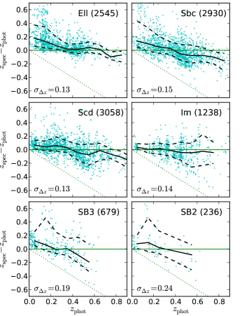
Figure 10: Photometric redshift errors in the source catalogue by template types (Ell, Sbc, Scd, Im, SB3, and SB2), as a function of the photometric redshift (the observable). The number in parenthesis indicates object counts. The median (bold solid line) and the 16 and 84 percentile range (bold dashed line) of $\Delta z$ is also shown. The photo-$z$ scatter is given as the standard deviation of $\Delta z$ from the median. Only 50 per cent of the points are shown for clarity. We impose a photo-$z$ quality cut by removing all SB2 and SB3 objects from our bias analysis, with $\lesssim 10$ per cent loss of objects.

Figure 10 shows the photometric redshift error for the source catalog, for each template type separately. The errors are displayed as a function of photo-$z$, i.e., the observable; this format also clearly displays the different features in photo-$z$ errors by template types. The dispersion around the median bias is quantified as

$$\sigma^{2}_{\Delta z}=\langle[\Delta z-{\rm median}(\Delta z)]^{2}\rangle\;,$$ (12)

and each panel shows $\sigma_{\Delta z}$ for that template type. The photo-$z$ failures constitute $\sim$2 per cent of the objects, which are not shown. The relative fraction of template types in the photo-$z$ sample show that approximately a quarter each are of the Ell, Sbc, and Scd galaxy types; about 10 per cent are of the Im-type, and $<$10 per cent are classified as either SB2 or SB3. The lens sample shows a similar distribution of galaxy types.

The galaxies classified as starburst (SB2 and SB3) SED types show the largest photo-$z$ errors. Our photo-$z$ quality cut discards the SB2 and SB3 template type objects along with the $\sim$2 per cent photo-$z$ failures. We lose $\lesssim$10 per cent of our sample with this cut.

For the remaining four template types, the width of the photo-$z$ error (dashed lines, Fig. 10) in general becomes narrower as the galaxy becomes brighter, down to $\sigma_{\Delta z}=0.09$ for $r<20.5$. In general, it is believed that red galaxies (Ell) have better photometric redshift accuracies compared to the bluer galaxy types, due to the high contrast below and above the (rest-frame) 4000Å break. However, this statement is only true when there is a strong photometric detection in the bands above and below the break. The large photo-$z$ errors in the Ell and Sbc samples at $z_{\rm phot}<0.2$ are due to noisy photometry; this broad dispersion stems from the fact that photo-$z$ depends on the colour difference between the $g$ and the $ri$ bands at low $z_{\rm phot}$ to probe the $4000\AA$ break; but at dim $ri$ magnitudes, the $g$ magnitudes for the red Ell and Sbc galaxies are even dimmer, resulting in a photo-$z$ fit that is highly sensitive to noise.

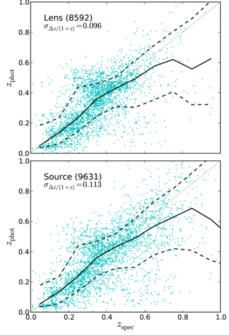
Figure 11: Photo-$z$ as a function of spectroscopic redshifts for the SDSS lens (top) and source (bottom) catalogues, after photo-$z$ quality cuts have been applied. The median (bold solid line) and the 16 and 84 percentile range (bold dashed line) of $\Delta z$ is also shown. The error uncertainty is given as the standard deviation of $\Delta z/(1+z_{\rm spec})$. Only 33 per cent of the points are shown for clarity.

Figure 11 shows results for the full samples (all templates) using the more standard format for comparison with other photo-$z$ literature: the photo-$z$’s are shown as a function of the true redshift, and scatter is quantified as

$$\sigma_{\Delta z/(1+z)}^{2}\equiv{\rm var}[\Delta z/(1+z_{\rm spec})],$$ (13)

where $\Delta z\equiv z_{\rm phot}-z_{\rm spec}$. The photo-$z$ error is large, where $\sigma_{\Delta z/(1+z)}=0.096$ and 0.113 for the lens and the source sample, respectively, averaged over the whole sample. In comparison, ZEBRA template-fitting photo-$z$’s in Feldmann et al. (2006) achieve accuracies of $\sigma_{\Delta z/(1+z)}<0.03$ when applied to $I_{AB}<22.5$ COSMOS galaxies with $u^{*}BVg^{\prime}r^{\prime}i^{\prime}z^{\prime}K_{s}$ photometry, thus suggesting that the systematic floor due to limitations of the code and template set are low, and our errorbars are dominated by photometric noise. We find that the scatter is a function of magnitude, and degrades rapidly for $r>21$. For our source catalogue, however, the degradation at the faint end is not so severe ($\sigma_{\Delta z/(1+z)}\sim 0.13$ for $21<r<21.8$); this implies that the better resolution required for the source sample yields more reliable photometry.

The photo-$z$ scatter is asymmetric about the median. In particular, Figure 11 shows bimodality in the photo-$z$ distribution for $0.2<z_{\rm spec}\lesssim 0.4$. This feature is seen in all template types, and is an artifact of the gap between the $g$ and $r$-bands at $5440$Å, or equivalently, when the 4000Å break transitions from $g$ into $r$ at $z\sim 0.36$. The gap between the $g$ and $r$ bands causes uncertainty in the photometric redshift when $z_{\rm spec}=0.36$ even with perfect photometry; with high photometric noise, the error in the photo-$z$ becomes bimodal centered at this redshift.

5.2 Uncertainty in template types

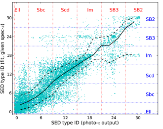
Figure 12: SED template type uncertainty in the source catalogue (the lens catalogue show similar scatter). The ordinate is the “true” template ID, while the abscissa is the best template type estimate derived from the photo-$z$ run, and is our observable. The thick solid line and thick dashed lines show the median and the upper/lower 68 percentile scatter, respectively. The 6 basic CWW+Kinney template types correspond to template type IDs 0, 6, 12, $\ldots$ 30, with 5 interpolated SED templates in between. Our SED type classification bins are delineated by the straight, dotted lines. (The points are shown with random fractions of $\in[-0.5,0.5)$ added to better illustrate the density; the template type IDs are all integers.)

It is important to understand the error in template type designation, not only because we define our photo-$z$ quality cut based upon template type, but also because we want to understand and minimise the errors in $k$-correction (Sec. 4.3) and stellar mass estimates (Sec. 6.2.1). Figure 12 shows the template designation errors for the source catalogue. The “true” template types were determined by asking ZEBRA to fit to the best template type, given the known $z_{\rm spec}$, and is plotted on the vertical axis; the horizontal axis is the observable (the template type derived from photometry alone, when determining the photo-$z$). There are 5 interpolated SED templates in between the 6 basic CWW+Kinney template types; our SED type classification bins are delineated by the straight, dotted lines.

The median of the scatter lies on the slope $=1$ line, and the scatter width from the median in the range of Ell/Sbc/Scd/Im SED types is $\pm$ 3 units, which is approximately the half-width of the template type bins. Hence we see that the template type error is reasonably small for the chosen template categorisation. In contrast, very few objects fit to the interpolation between Im to SB2 or SB2 to SB3 types, with large uncertainty in the template types in these bins. The lens catalogue template type uncertainty show similar scatter.

However, even when using the spectroscopic redshifts, it is possible to have the wrong template, either because the template set may not describe the true galaxy SED, or due to the relatively large noise in the magnitudes which may cause the selection of the wrong template even when given the true redshift. This additional template type uncertainty is not accounted for in Fig. 12.

6 Bias in Luminosity and Stellar Mass

To obtain a weak lensing signal with sufficient signal to noise, lens galaxies with similar properties (such as luminosity and stellar mass) are stacked. Absolute magnitudes and stellar mass, used to assign lens galaxies to each stack, inherit scatter from photo-$z$ errors. With our lens calibration set we can measure this scatter, and use the width of the scatter to determine the binning resolution for stacking. Moreover we can test for biases in the absolute magnitudes and stellar masses, and figure out how to shift our bins around to account for this type of error.

6.1 Absolute magnitude

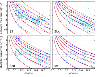
Figure 13: The theoretical ${}^{0.3}\!M_{r}$ absolute magnitude error curves (distance modulus $+$ $k$-correction) for objects at $z_{\rm spec}$$=0.1,0.2,$ …, $0.6$ (solid curves, from bottom to top), as a function of $z_{\rm phot}$, for each template types (Ell, Sbc, Scd, Im). The dashed line is the distance modulus component alone. If the photo-$z$ is below the spec-$z$ (top half of each panel), the estimated absolute magnitude is too large (fainter) than the real magnitude. The correction is more severe at smaller photo-$z$’s. The points show distribution of objects from our photometric lens catalogue ($r<21$).

The bias in absolute luminosity due to photo-$z$ errors is a combination of two effects: the error in the luminosity distance, and in the $k$-correction (Sec. 4.3). All magnitudes are $k$-corrected according to SED template types. We define our absolute magnitude band as the $r$ magnitude redshifted to $z=0.3$ (${}^{0.3}\!M_{r}$), so that in Eq. (10), $R=R^{\prime}=r$, and $z_{0}=0.3$, and where the observed $r$ magnitude was chosen for its high $S/N$. These choices minimise the degree of $k$-correction for our lens sample, and most of the correction is dominated by the distance modulus, as demonstrated in Figure 13. Here, the theoretical absolute magnitude errors in ${}^{0.3}\!M_{r}$ (distance modulus $+$ $k$-correction) are shown in solid curves, for objects at $z_{\rm spec}$$=0.1,0.2,$ …, $0.6$, as a function of $z_{\rm phot}$. The dashed lines show the magnitude modification from the distance modulus component alone; the fact that they nearly coincide with the solid lines indicates that the distance modulus error is more important than the uncertainty in $k$-corrections. The points show the distribution of galaxies from our photometric lens catalogue ($r<21$). Although the $k$-correction is in general small, it becomes somewhat more significant for Ell objects at high $z_{\rm phot}$ or $z_{\rm spec}$.

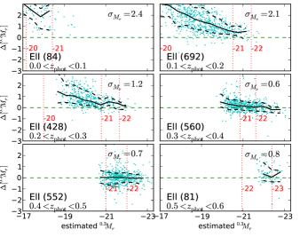
Figure 14: Absolute magnitude bias due to redshift errors, in $z_{\rm phot}$ and ${}^{0.3}\!M_{r}$ bins, for the Ell SED type. The 6 panels correspond to different $z_{\rm phot}$ bins; the points show individual objects, while the thick solid and dashed lines are the median and 16/84 percentile of the points in a given ${}^{0.3}\!M_{r}$ bin. The vertical dotted lines correspond to the true ${}^{0.3}\!M_{r}$ of the median $\Delta[^{0.3}\!M_{r}]$, and these lines are labeled with the true ${}^{0.3}\!M_{r}$ values. The large bias and scatter at low photo-$z$ ($z_{\rm phot}$$<0.2$), low luminosity (${}^{0.3}\!M_{r}>-21$) bins are due to the large photo-$z$ errors in those bins for this SED type. The numbers in parenthesis indicate the galaxy counts in the panel.

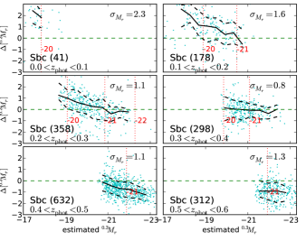
Figure 15: Absolute magnitude bias due to redshift errors, in $z_{\rm phot}$ and ${}^{0.3}\!M_{r}$ bins, for the Sbc SED type (see Fig. 14 caption for description).

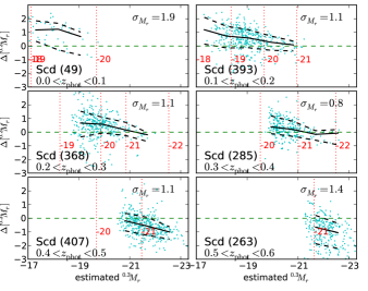
Figure 16: Absolute magnitude bias due to redshift errors, in $z_{\rm phot}$ and ${}^{0.3}\!M_{r}$ bins, for the Scd SED type (see Fig. 14 caption for description).

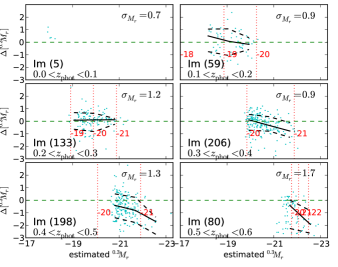
Figure 17: Absolute magnitude bias due to redshift errors, in $z_{\rm phot}$ and ${}^{0.3}\!M_{r}$ bins, for the Im SED type (see Fig. 14 caption for description).

The size of the scatter in ${}^{0.3}\!M_{r}$ dictates the appropriate luminosity binning width. We further bin the lens objects by redshift bins of width $\Delta z_{\rm phot}=0.1$, up to $z_{\rm phot}=0.6$, to determine the binning width as a function of $z_{\rm phot}$ and SED type. The actual distribution of absolute magnitude error $\Delta[^{0.3}\!M_{r}]\equiv\ ^{0.3}\!M_{r}(z_{\rm phot})-\ ^{0.3}\!M_{r}(z_{\rm true})$ is determined by the photo-$z$ distribution and error distribution of the photometric lens sample. Figures 14 through 17 show the median and scatter in the error $\Delta[^{0.3}\!M_{r}]$ for the four SED template types $T$ that we use for our analysis, as a function of the estimated absolute magnitude ${}^{0.3}\!M_{r}(z_{\rm phot})$ (the observable), where sub-panels in each figure are binned by the photometric redshifts.

The smallest scatter is seen in the Ell type galaxies at high redshift ($z>0.3$) and bright absolute magnitude (${}^{0.3}\!M_{r}(z_{\rm phot})<-20$). This is the binning range most relevant to current SDSS LRG studies. These bright, red galaxies show the smallest $\Delta[^{0.3}\!M_{r}]$ scatter of $\sigma_{M_{r}}\sim 0.7$ magnitude from the median. The large scatter in the low $z_{\rm phot}$, low luminosity region, $\Delta[^{0.3}\!M_{r}]\gtrsim 2$, comes from the broad redshift uncertainty in the red SED types at low $r$ magnitude, as discussed in Sec. 5.1. Unlike LRGs, dim red objects with ${}^{0.3}\!M_{r}(z_{\rm phot})\sim^{0.3}\!M_{r}(z_{\rm spec})>-21$ do not have reliable magnitudes, because the photo-$z$ errors are worse (Sec. 5.1). For other SED types and photo-$z$ bins, a typical magnitude scatter is about $\sigma_{M_{r}}\sim$1, and so the bin size cannot be much smaller than this. We also note that where the calibration sample distribution is sparse, the binning cannot be reliable. For this reason, the redshift bin $0<z_{\rm phot}<0.1$ is probably best omitted, for lenses of all SED types.

The vertical dotted lines in Figures 14–17 show where stacking the lens galaxies by absolute magnitude binning would be meaningful where the average $\sigma_{{}^{0.3}\!M_{r}}$ (averaged over the photo-$z$ bin) are shown in each panel. The brightest bins (${}^{0.3}\!M_{r}<-21$) are accessible to the Ell and Sbc types at high $z_{\rm phot}$, where the faint end (${}^{0.3}\!M_{r}>-19$) are accessible to Scd and Im objects in the $0.1<z_{\rm phot}<0.2$ bin.

An additional consideration in comparing magnitudes across different redshifts is the luminosity evolution. Between the lowest and highest redshift bin, evolution accounts for a difference in $\sim$0.5 magnitudes. This is estimated according to the luminosity function (LF) evolution, based on several LF studies in a similar redshift range (Wolf et al., 2003; Giallongo et al., 2005; Willmer et al., 2006; Brown et al., 2007; Faber et al., 2007). We adopt $Q=1.2$ mag/redshift for all templates, which appears to be consistent with all of these studies, and where $Q$ is the redshift evolution slope as defined in

$$M_{*}(z_{0})=M_{*}(z)+(z-z_{0})Q$$ (14)

where $M_{*}$ is the magnitude corresponding to $L_{*}$ in the luminosity function, $z$ is the object redshift, and $z_{0}$ is the standard redshift to which we normalise our magnitude binning. These studies are based on $B$-band luminosities, but ${}^{0.3}\!r$ and $B$ are close enough (they partially overlap at 4300–4700Å); hence the correction from the colour evolution is expected to be small. If we make the simplifying assumption that the luminosity rank ordering does not mix as the luminosity function evolves, then we can define magnitude bins that shift according to the slope $Q$ as a rough approximation to the luminosity evolution. This correction is a small effect compared to the shifts induced by photo-$z$ error bias.

6.2 Stellar mass

6.2.1 Estimating stellar mass

Stellar mass can be estimated from the combination of (1) rest-frame colours and (2) absolute magnitude (discussed above in Sec. 6.1), using correlations by Bell et al. (2003) (via an intermediate step of estimating a stellar mass-to-light ratio, $M_{*}/L$). The colour—$M_{*}/L$ relation is defined using the rest frame colour in Bell et al. (2003); and SED types are used to convert colours and magnitudes into the rest frame. As excessive $k$-corrections are susceptible to errors in photo-$z$ and SED types, we choose the optimal observed band which minimises the $k$-correction to the rest frame band. We $k$-correct the observed $i$ magnitude into the ${}^{0.0}\!r$ band rest-frame absolute magnitude and the observed $r-i$ colour to ${}^{0.0}(g-r)$ (Sec. 4.3). The ${}^{0.0}\!r$ band rest-frame is chosen since its wavelength range approximately corresponds to that of the observed $i$ band at the lens median redshift of $z_{0}=0.3$, which is the reddest band available in SDSS with high photometric S/N (red luminosities require less correction to the $M_{*}/L$ ratio). Similarly the ${}^{0.0}(g-r)$ colour is chosen for the higher S/N in the observed $r$ and $i$ bands. Then, the $M_{*}/L$ ratio is obtained from Table 7 of Bell et al. (2003),

$$\log_{10}(M_{*}/L_{r})=-0.306+1.097\;[^{0.0}(g-r)]$$ (15)

where $M_{*}/L_{r}$ (stellar mass $M_{*}$ to ${}^{0.0}r$-band luminosity ratio) is in solar units. The $r$ band luminosity in solar units is

$$\log_{10}L_{r}=-0.4\;(^{0.0}\!M_{r}-4.64)$$ (16)

where $(M_{r})_{\odot}=4.64$ is the $r$-band absolute AB magnitude of the Sun (Blanton & Roweis, 2007). Hence the stellar mass in solar units is

$$\log_{10}M_{*}=1.550+1.097\;[^{0.0}(g-r)]-0.4\;[^{0.0}\!M_{r}].$$ (17)

These numbers quoted above are based on a diet Salpeter IMF; for future science work we can modify for this by rescaling all stellar masses by a constant factor.

We now consider biases in these stellar masses. We start with biases in the intermediate step of constructing the stellar mass-to-light ratio.

6.2.2 Bias in stellar mass-to-light ratio

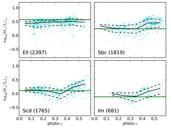
Figure 18: The scatter in the stellar mass-to-light ratio ($M_{*}/L$) with respect to rest-frame $r$-band luminosity in solar units, as a function of photo-$z$, for the different SED types, determined from photo-$z$ fitting. The thick horizontal line shows the theoretical $M_{*}/L$ based on the rest-frame colour, and is constant for a given SED type. The points are the $M_{*}/L$ estimated from the “true” template type (best-fit template given the spec-$z$) $k$-corrected using the true redshift ($z_{\rm spec}$), and the solid/dashed lines show the median and 68 percentile scatter, respectively. The $M_{*}/L$ determined from $z_{\rm phot}$ has intrinsic scatter of $\sim$0.1 dex (not shown). The scatter in $M_{*}/L$ is small compared to the bias in the luminosity $L$.

In this section, we consider errors in the inferred $M_{*}/L$ using photo-$z$, starting from the basic assumption that these are significantly larger than intrinsic uncertainties in the Bell et al. (2003) prescription for estimating stellar mass when using spectroscopic redshifts. This statement ignores underlying uncertainties in the stellar IMF, which plague all stellar mass estimates.

There is very little bias and scatter when we plot the $M_{*}/L$ obtained from the rest-frame ${}^{0.0}(g-r)$ colour by SED template types. This is because for a given SED template, the rest-frame colour is a constant. Instead, we take the “true” template type and $k$-correct using the true redshift. The $k$-corrected colour ${}^{0.0}(g-r)$, and hence the derived $M_{*}/L$, then show some bias and scatter, as seen in Figure 18. The constant (as a function of $z_{\rm phot}$) predicted $M_{*}/L$ for the given template type is shown for comparison. The points show the distribution of the lens catalogue objects, and the solid/dashed lines show the median and 68 percentile scatter, respectively. There is still little variation in the $M_{*}/L$ evident, because the rest-frame colours are identical for a given template type, and the “true” template type deviates little from the estimated one. The magnitude of the scatter shown is similar to the uncertainty in the $M_{*}/L$ relation (Eq. 15) itself, which is $\sim 0.1$ dex (Bell et al., 2003). The true errors in $M_{*}/L$ might be expected to be larger than that shown here, given that the actual galaxy SED is unknown. However, we expect the error in the luminosity to dominate, discussed below.

6.2.3 Bias in stellar mass

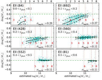
Figure 19: Stellar mass errors $\Delta\log_{10}[M_{*}/M_{\odot}]\equiv\log_{10}[M_{*}/M_{\odot}](z_{\rm phot})-\log_{10}[M_{*}/M_{\odot}](z_{\rm spec})$ in the Ell SED type, as a function of the estimated stellar mass based on $z_{\rm phot}$ (the observable). The distribution of the lens catalogue are plotted as points, where the median and 68 percentile scatter are shown as the thick solid and dashed lines, respectively. Each panel correspond to different $z_{\rm phot}$ bins. The top axis of the top panels show the nominal stellar mass bin of 0.3 dex, or where the bin is twice as massive as the previous one. The vertical dotted lines show the bias-corrected binning.

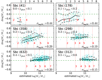
Figure 20: Stellar mass errors in the Sbc SED type.

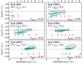
Figure 21: Stellar mass errors in the Scd SED type.

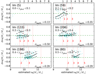
Figure 22: Stellar mass errors in the Im SED type.

While the scatter in $M_{*}/L$ is of order $0.1\sim 0.2$ dex, the scatter in the luminosity is $\sim 0.4$ dex (converted from $\sim$1 mag scatter, see Eq. 16), mostly dominated by the distance modulus (Sec. 6.1). Figures 19–22 show the bias and scatter in stellar mass estimate in the four template types, as a function of estimated stellar mass, for the 6 photo-$z$ bins. The errors (vertical axis) are plotted as a function of estimated stellar magnitudes $\log_{10}[M_{*}/M_{\odot}](z_{\rm phot})$ (the observable), where the nominal stellar mass bins are in widths of 0.3 dex (i.e, each bin is twice as massive as the previous bin). These bins are labeled by the index 1 through 8, as seen on the topmost panels in each Figure. The vertical dotted line, labeled by stellar mass bin numbers, are the corrected stellar masses based on the median values.

We see the general trend in the absolute luminosity bias and scatter repeated in these plots, e.g., the Ell types show small scatter at high stellar mass and high $z_{\rm phot}$, and the lowest $z_{\rm phot}$ bin ($0<z_{\rm phot}<0.1$) is too sparse. The $\log_{10}[M_{*}/M_{\odot}]$ scatter $\sigma_{\log M_{*}}$, which is defined with respect to the median, is shown in each plot, and indicates small scatter for most bins. In fact, most bins show scatter smaller than the nominal 0.3 dex stellar mass bin.

We note that previous studies (e.g., Dutton et al. (2010)) have compared the photometry-based stellar mass estimate employed here with spectra-based estimates. On average, the two agree for higher stellar masses, but deviate systematically at lower stellar mass. Such systematic deviation can be corrected accordingly with a stellar-mass dependent correction.

7 Bias in the gravitational lensing signal

With these photometric redshifts, their scatter and their effects on stellar mass and absolute magnitudes quantified, we can turn to the bias and scatter induced in the gravitational lensing signal due to photo-$z$ use for sources and lenses. As the conversion of lensing shear to mass depends upon the redshifts of the lens and source (see Eq. 1), errors in these redshifts propagate into errors in the weak lensing measurements. We consider three cases, (a) the lens redshift is known and photo-$z$ is only used for the source, (b) the source redshift is known and photo-$z$ is only used for the lens, and (c) photo-$z$’s are used for both lens and source. We deal with these in turn below, focusing on biases in the lensing signal calibration; in principle, there is also a blurring of information in the transverse direction once photo-$z$ are used for lenses; however, a typical 10 per cent photo-$z$ error does not have a significant effect on the shape of the lensing profiles, so we neglect this effect here. We begin by reviewing and then expanding upon the methods by Mandelbaum et al. (2008) to calculate lensing bias.

7.1 Methods

7.1.1 Bias

In the absence of photo-$z$ errors, the observed lensing tangential shear $\gamma_{t}$ can be related to the lens surface density contrast $\Delta\Sigma$ via

$$\Delta\Sigma=\Sigma_{c}\gamma_{t}$$ (18)

where the proportionality constant, the critical surface density, was defined in Eq. (1).

The redshift calibration bias is the misestimation of $\Delta\Sigma$ due to the photo-$z$ scatter. To estimate this bias, we first consider the method of estimating $\Delta\Sigma$, via a weight-average over the tangential component of the measured source galaxy shapes $\tilde{\gamma}_{t}^{(j)}$,

$$\widetilde{\Delta\Sigma}=\frac{\sum_{j}\tilde{w}_{j}\tilde{\gamma}_{t}^{(j)}\widetilde{\Sigma}_{c,j}}{\sum_{j}\tilde{w}_{j}}\;.$$ (19)

Here, the summation is over $j$ lens-source pairs, $\Sigma_{c,j}$ is the critical mass density for the $j$th lens-source pair, and the tilde indicates estimated values (using photo-$z$’s where applicable). The optimal weight is

$$\tilde{w}_{j}=\frac{1}{\widetilde{\Sigma}_{c,j}^{2}\,(e^{2}_{\rm rms}+\sigma_{e,j}^{2})}.$$ (20)

The quantities added in quadrature are $e_{\rm rms}$, the shape noise of the source ensemble, and $\sigma_{e,j}$, the shape measurement error of the $j$th galaxy (per single component of the shear). Assuming that the only calibration bias occurs through the use of photo-$z$ via the quantity $\widetilde{\Sigma}_{c}$, the redshift calibration bias $b_{z}$ is the ratio of $\widetilde{\Delta\Sigma}$ to the true signal $\Delta\Sigma$. By substituting $\tilde{\gamma}_{t}^{(j)}=\Delta\Sigma\Sigma^{-1}_{c,j}$, we find

$$b_{z}(z_{\rm lens})+1\equiv\frac{\widetilde{\Delta\Sigma}}{\Delta\Sigma}=\frac{\sum_{j}\tilde{w}_{j}\Sigma^{-1}_{c,j}\widetilde{\Sigma}_{c,j}}{\sum_{j}\tilde{w}_{j}}\;,$$ (21)

the weighted sum of the ratio of the estimated to true critical surface density.

In the actual bias estimation, each galaxy $j$ is further weighted to “smooth” out the LSS in the calibration sample. To do so, we fit the redshift histogram to the analytic curve Eq. (3), as seen in Figs. 8 and 7; the LSS weight for all galaxies in a particular histogram bin $i$ is then the ratio of the number of galaxies according to the fit distribution, to the real number of galaxies, i.e., $w_{\rm LSS}=N^{\rm(model)}_{i}/N_{i}$ (Mandelbaum et al., 2008). The analytic curve is fit separately for every calibration subsample that is used.

The bias (Eq. 21) is for a single lens redshift. If we want to estimate the average bias from using photo-$z$ for $z_{\rm src}$ over all lenses with known $z_{\rm lens}$, we need to average over the lens redshift distribution, including source weight factors,

$$\langle b_{z}\rangle=\frac{\int\mathrm{d}z_{\rm lens}\,p(z_{\rm lens})\tilde{w}_{l}(z_{\rm lens})b_{z}(z_{\rm lens})}{\int\mathrm{d}z_{\rm lens}\,p(z_{\rm lens})\tilde{w_{l}}(z_{\rm lens})}\;.$$ (22)

The weight for a given lens redshift $\tilde{w}_{l}(z_{\rm lens})$ is

$$\tilde{w}_{l}(z_{\rm lens})=D^{-2}_{L}(1+z_{\rm lens})^{-2}\,\sum_{k}\tilde{w}_{k}\;.$$ (23)

Here the summation is over all source galaxies $k$ estimated to be beyond the lens redshift $z_{\rm lens}$, and $z_{\rm lens}$ may be spectroscopic or photometric. The reason for the prefactors before the summation is that our method of estimating these sums using a calibration sample of fixed area does not really correspond to how lensing signals are actually measured. Typically they are estimated within some fixed physical or comoving aperture, which means that lenses at lower redshift will use sources from an effectively larger area on the sky, and therefore get greater weight according to the square of that angular diameter distance to the lens redshift. The factor of $(1+z_{\rm lens})^{-2}$ assumes the use of a fixed comoving aperture. Note that this effect was incorrectly neglected in the previous analysis (eq. 6 of Mandelbaum et al. 2008). Fortunately, it is only significant when averaging over a broad lens redshift distribution. In subsequent papers relying on the Mandelbaum et al. (2008) lensing signal calibrations, including Mandelbaum et al. (2008); Reyes et al. (2008); Mandelbaum et al. (2009, 2010); Schulz et al. (2010), the change in the lensing signal calibration when including this additional redshift weighting factor is typically $2$ per cent, which is approximately the size of the quoted systematic uncertainty in the redshift calibration, and typically  20 per cent of the statistical error.

7.1.2 Source-lens pair (statistical) incompleteness

The bias as described above does not indicate the statistical loss in the number of valid source-lens pairs, or in the deviation from optimal weighting due to the use of photo-$z$. Such contributions can be described in terms of the purity and completeness of the lens-source pairs, and the change in weights from using photo-$z$ instead of the true redshift. Purity is the fraction of lens-source pairs that are truly lensed with all “valid” pairs based on photo-$z$, where each pair is weighted according to Eq. (20). Completeness is the ratio of the sum of all weights of the lens-source pair ensemble, calculated based on photo-$z$ to that based on the true redshift. The loss of statistics due to low purity and completeness translates to higher uncertainty (variance) in $\Delta\Sigma$. The efficiency is defined as the ratio of the variances, where the smaller, ideal variance is attained when all redshifts are known, and the estimated variance obtained from using photo-$z$’s is always larger than the ideal variance due to the two previous issues (low purity and/or completeness) plus deviation of the weighting from the optimal weighting. This efficiency is given by (Mandelbaum et al., 2008)

$$\frac{{\rm Ideal\ Var}(\Delta\Sigma)}{{\rm Real\ Var}(\Delta\Sigma)}=\frac{\left(\sum\sqrt{\tilde{w}w}\right)^{2}}{\left(\sum{w}\right)\left(\sum{\tilde{w}}\right)}$$ (24)

where the weights are defined in Eq. (20), and the tilde indicates values estimated based on photo-$z$’s. These will be illustrated for the case of both source and lens photo-$z$ (§7.4) below.

7.1.3 Bias uncertainties from LSS

The uncertainty in the calibration bias estimated using Eq. (21) is determined not only by the size of the calibration sample (Poisson statistics) but also by its LSS fluctuations. To estimate the size of this uncertainty, Mandelbaum et al. (2008) used a modified bootstrap resampling method to estimate the uncertainty in the true source redshift distribution, and hence in the bias curve, $b_{z}(z_{\rm lens})$, where $z_{\rm lens}$ is known. In this paper, we take a simpler approach. Since we have several calibration subsamples representing independent realizations of LSS, we obtain a bias curve $b_{z}(z_{\rm lens})$ for each subsample, take their average as the bias, and the standard deviation of the mean as the systematic uncertainty due to LSS (see, e.g. Fig.  23).

Given the formalism described in this section, we now turn to the case of source photo-$z$, lens photo-$z$, and both combined.

7.2 Lensing bias in source photo-$z$

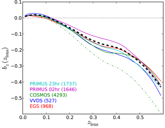
Figure 23: Lensing signal calibration bias from using photo-$z$ for $z_{\rm src}$, given a known lens redshift $z_{\rm lens}$. The thin solid lines show bias in the EGS, VVDS, COSMOS, PRIMUS-02hr and PRIMUS-23hr fields, and the weighted average of the 5 solid curves is shown as the thick dashed line. Of the 5 fields, the COSMOS field bias has been empirically corrected (see text); the pre-correction bias is shown as the thin dot-dashed line.

First, we consider the case where the lens redshifts are known to high accuracy, but the source redshifts rely on much more uncertain photo-$z$. Figure 23 shows the lensing bias $b_{z}(z_{\rm lens})$ for using photo-$z$ in the new SDSS source catalogue as a function of the known lens redshifts $z_{\rm lens}$. Bias for each the 5 source calibration subsamples (EGS, VVDS, COSMOS, PRIMUS-02hr and PRIMUS-23hr) are shown as thin solid lines. Of the 5 fields, the calibration bias in the COSMOS field has been empirically corrected to account for excessive sky noise, as will be described shortly. Prior to calculating the bias, all subsamples have the photo-$z$ quality cuts applied (Sec. 5.1), and the “excess” low-resolution galaxies have been omitted in the VVDS, PRIMUS-02hr and 23hr fields (Sec. 3.2.3). The bias $b_{z}(z_{\rm lens})$ can be as low as $-0.4$ at $z_{\rm lens}=0.5$, but the uncertainty in the bias is less than 0.03; i.e., $-0.40\pm 0.03$. In general, source photo-$z$’s with large scatter tend to pull the bias more negative.

As noted previously, it was impossible to augment the COSMOS sample to correct for the loss of observable galaxies due to excessively high sky noise (Sec. 3.2.1); instead, it is necessary to derive an empirical correction to the bias. The redshift calibration bias curve for the COSMOS calibration sample, before correction, can be seen as the dot-dashed line in Fig. 23; clearly it is quite discrepant compared to the other samples. We have empirically compensated for this effect using the following procedure: We used the fact that our PRIMUS-02hr and 23hr calibration samples are on stripe 82, where there are many SDSS observing runs with different conditions. Thus, we chose runs overlapping those two regions with seeing that is comparable to in the COSMOS region, but with two different values of sky noise: typical, and 20 per cent larger (as in the COSMOS region). We carry out the bias calculations independently for each of the observing runs with different conditions, including matching against the spectroscopic training sample, imposing the lensing quality cuts, and obtaining photo-$z$’s from the photometry. We calculate the resulting lensing signal bias $b_{z}(z_{\rm lens})$ from the photo-$z$’s for the two runs separately, and then use the difference between to two to correct for the COSMOS sample bias. It is reassuring that after applying this correction, the calibration bias for the COSMOS sample is reasonably consistent with that for the other four calibration samples.

7.3 Lensing bias in lens photo-$z$

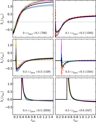
Figure 24: Bias in the gravitational lensing signal due to photo-$z$ usage for lens redshifts, as a function of known source redshift, $b_{z}(z_{\rm src})$. The different panels show $z_{\rm phot}$ bins of lens redshifts; the number in parenthesis indicates the number counts of galaxies in the spectroscopic lens calibration sample in this photo-$z$ bin. The thin lines are the biases in the six individual lens calibration subsamples, and the thick line is the overall bias from the combination of all calibration subsamples. The thin dashed line indicates the EGS sample before the deficient $z\sim 0.3$ bin has been corrected for (Sec. 7.3). We discard the lowest redshift bin, $0<z_{\rm phot}<0.1$, since the different calibration subsamples suggest inconsistent values for the calibration bias.

Next we calculate the bias in the gravitational lensing signal when the source redshift is known, but photo-$z$ is used for the lens redshift. Unlike the case above (Sec. 7.2) where $z_{\rm lens}$ is known but photo-$z$ is used for source redshifts, such a scenario is not relevant for real observations. However, this exercise will allow us to study the general response of the lensing bias $b_{z}$ to errors in lens photo-$z$, and may suggest certain scenarios in which using photo-$z$ for $z_{\rm lens}$ would be inadvisable. As this is just an exercise, we do not consider the purity, completeness and efficiency; only the lensing calibration bias is shown.

Figure 24 shows the bias $b_{z}(z_{\rm src})$ as a function of the known $z_{\rm src}$. We initially found that all calibration subsamples agree well except for EGS; this deviation was due to the lack of objects in the $z\sim 0.3$ bin, as discussed in Sec. 3.4. This discrepancy is easily remedied when the deficient bin in the EGS sample is replaced with, e.g., objects from the VVDS survey of the same redshift bin (both the original and corrected EGS biases are shown in the plot). Note that this correction was not required in Sec. 7.2 when using source photo-$z$. The observing conditions that affect the $r<21.8$ source calibration sample are not relevant to the lens $r<21$ sample because (a) it does not have resolution cuts, and hence is not affected by the variation in the seeing, and (b) it has a brighter flux limit, such that the sky noise has minimal effect on the number counts (Sec. 3.2.2).

For all $z_{\rm lens}$ bins, we see that the lensing bias converges at high $z_{\rm src}$ to a reasonable value for most $z_{\rm phot}$ bins except the lowest lens redshift bin $0<z_{\rm phot}<0.1$. We also see that the bias $b_{z}(z_{\rm src})$ varies rapidly close to the lens redshift, and also shows the largest difference between the calibration subsamples (perhaps reflecting a sensitivity to LSS fluctuations in the lens number density or overall characteristics such as domination by red vs. blue galaxies). The characteristic width of this high-variation region is approximately $\Delta z_{\rm phot}\sim 0.1$, implying that a minimum lens-source separation of 0.1 in redshift can help stabilise the bias and minimize its associated systematic uncertainty. In reality, with only photo-$z$ for both $z_{\rm lens}$ and $z_{\rm src}$, such a clean cut is impossible, and there may not be significant benefit when applying a minimum separation cut. We explore this issue further in the next section.

7.4 Lensing bias, lens and source photo-$z$

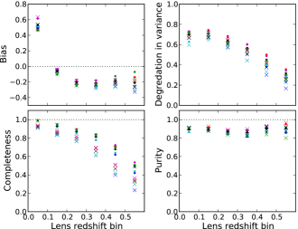
Figure 25: Top left: Bias $b_{z}$ in the galaxy-galaxy lensing signal due to photo-$z$ usage for both the lens and source. The lens galaxies have been binned according to photo-$z$ bin width of $\Delta z_{\rm phot}=0.1$. All 5 calibration subsamples (EGS, VVDS, COSMOS, PRIMUS-02hr and PRIMUS-23hr) have been plotted to show the LSS-induced scatter. Dots: no pair rejection applied. Crosses: Minimum photo-$z$ separation of 0.1 between lens and source required. Top right: Efficiency (degradation in variance), as defined in Sec. 7.1.2. Bottom left and right panels: Completeness and purity, respectively, as defined in Sec. 7.1.2. The weighting scheme keeps the lensing signal relatively pure, while the degradation in the variance (statistical loss) comes mostly from the incompleteness of the valid lens-source pairs due to the use of photo-$z$ errors.

Table 3: Lensing signal bias and its uncertainty, for photo-$z$ lens and source redshifts, from the bias panel in Figure 25.

Lens photo-$z$ bin	Lensing bias	(COSMOS noise bias)
Using all samples
0.05	0.513 $\pm$ 0.055	(-0.027)
0.15	-0.061 $\pm$ 0.025	(-0.035)
0.25	-0.211 $\pm$ 0.027	(-0.048)
0.35	-0.227 $\pm$ 0.029	(-0.068)
0.45	-0.178 $\pm$ 0.034	(-0.105)
0.55	-0.183 $\pm$ 0.069	(-0.167)
With minimum photo-$z$ separation of 0.1
0.05	0.521 $\pm$ 0.058	(-0.027)
0.15	-0.063 $\pm$ 0.019	(-0.041)
0.25	-0.219 $\pm$ 0.025	(-0.049)
0.35	-0.244 $\pm$ 0.031	(-0.074)
0.45	-0.220 $\pm$ 0.033	(-0.115)
0.55	-0.249 $\pm$ 0.062	(-0.167)

One of the main goals of this paper is to lay the groundwork for galaxy-galaxy lensing using photo-$z$ for sources and lenses. As mentioned in the introduction, this will dramatically increase the range of SDSS galaxies accessible for study with galaxy-galaxy lensing, both in the direction of lower luminosity at fixed redshift, and also going to higher redshift samples at fixed luminosity. Figure 25 shows the lensing signal bias, efficiency, completeness and purity when photo-$z$ lens-source pairs are used. The bias values have been tabulated in Table 3. The lens galaxies have been binned by photo-$z$ only. All 5 calibration subsamples (EGS, VVDS, COSMOS, PRIMUS-02hr and 23hr) have been plotted to show the LSS-induced scatter. Each subsample has been modified as follows: (1) the COSMOS sample has been corrected for the skynoise-induced excess bias (Sec. 7.2), where the excess bias is tabulated in Table 3; (2) the modified EGS lens sample has been used (Sec. 7.3) to calculate the bias in EGS; and (3) the low resolution objects in the stripe 82 samples (VVDS, PRIMUS-02hr and PRIMUS-23hr) have been removed from the source sample (Sec. 3.2.3). Although not shown here, further binning of the lens objects (reflecting the stacking scheme, e.g. based on stellar mass or luminosity) would be necessary to estimate the bias for any particular science application.

These panels again show that calibrating the lowest redshift bin for the lens can be unreliable, as demonstrated by the large variance in the bias $b_{z}$ between the different calibration samples. The highest redshift bin have a significant scatter in the bias among the subsamples which comes from the skynoise correction (applied to the COSMOS sample). Otherwise, the bias correction is $\sim$20 per cent, with the subsamples showing agreement to 4 per cent scatter. As we go to higher lens redshift bins, the efficiency and completeness drops, but not too significantly. Purity (at 90 per cent) remains high in all lens redshift bins. Application of lens-source photo-$z$ separation requirement does not have a significant effect on the lensing bias or its scatter, while completeness (and hence efficiency) drops. This indicates that the minimum photo-$z$ separation cut as implemented here is unnecessary. We interpret this to mean that our weighting scheme (Eq. 20) sufficiently down-weights nearby lens-source pairs that their potentially strong calibration biases do not lead to significant uncertainty in the calibration bias.

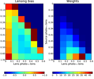
Figure 26: Left: Lensing signal bias, as a function of photo-$z$ bins in both lenses and sources. The lens bins are split into 0.1 redshift intervals, while the source bins are split into 9 equal parts. Right: Lensing signal weights in each of the lens/source bins. The highest source photo-$z$ bins carry the most weight at any lens photo-$z$ bin. The lowest lens photo-$z$ bins, as well as the bins where lens photo-$z$ is near the source photo-$z$, are highly biased, but carry very little weight.

Figure 26 shows the lensing bias as a function of lens and source photo-$z$ bin. The lens photo-$z$ bins are in 0.1 intervals, while the source photo-$z$ calibration sample was split into 9 equal parts of approximately 1000 galaxies each. The photo-$z$ bin edges are given in the vertical axis of the figure. The highly-biased bins generally have low weighting; the lowest lens photo-$z$ bin is highly biased, and carries no weight (hence also rendering the calibration unreliable), and similarly for bins where lens photo-$z$’s are close to source photo-$z$’s. This figure clearly demonstrates that the highest source photo-$z$ bin carries the most weight at any lens photo-$z$ bin, and also has the lowest bias (except for the lowest lens photo-$z$ bin). This is expected, because as the source redshift is well above the lens redshift, the weight $\propto\Sigma_{\rm crit}^{-2}$ increases, while the the lensing strength $\Sigma_{\rm crit}^{-1}$ becomes less sensitive to the source redshift errors.

8 Summary and conclusion

In this paper, we have sought to address technical issues required to use photometric redshifts for both lenses and sources in galaxy-galaxy lensing analyses without incurring significant systematic error.

To this end, we have obtained photometric redshifts for SDSS DR8 5-band photometry, using the template-based photo-$z$ code ZEBRA. Multiple readily available and self-generated photo-$z$ catalogues were perused and compared to optimize the photo-$z$ according to the key science goals of the catalogue, galaxy-galaxy lensing, which led us to choose a method with minimal photo-$z$ scatter for galaxies with $z_{\rm phot}>0.1$ (which dominate such analyses). The underlying assumption is that with a calibration sample of sufficient size to characterize the bias and scatter, any photo-$z$ biases can simply be calibrated out, so they should not figure into the choice of photo-$z$ method (provided that they are not so pathological as to make the problem of calibrating them out with a reasonable size calibration sample intractable).

To measure the photo-$z$ biases and scatter, a calibration set was required. Tests of the calibration set, and corrections for exceptional observing conditions, were required to ensure that its photo-$z$ scatters and biases accurately represent those of the full SDSS DR8 lensing and source samples. The calibration sample was drawn from several effectively flux-limited spectroscopic samples (six for the shallower lens sample, five for the deeper source sample) consisting of $\sim$9k galaxies overlapping the SDSS footprint.

The measured photo-$z$ bias and scatter allowed estimates of their contributions to bias in observed galaxy-galaxy lensing signals. We considered source and lens photo-$z$ separately, with emphasis on the newer application to SDSS, lens photo-$z$. The use of photo-$z$’s for source redshifts (in addition to lens spectroscopic redshifts) allows for gravitational lensing signal calibration that is more precise than using an assumed redshift distribution, and allows for selection of specific source subsamples (e.g., brighter or fainter, or with some lens-source separation). For a known lens redshift, we estimate that the lensing tangential shear can be converted to surface mass density with an accuracy of 2 per cent. Using photo-$z$’s for lenses will make lenses available at higher redshifts (out to $z\sim 0.5$, limited to red galaxies) and dimmer magnitudes (down to $r\sim 21$ or ${}^{0.3}\!M_{r}\sim-19$, limited to blue), an increase of factors of at least ten compared to SDSS spectroscopic samples. Rather than lens samples with several tens of thousands of galaxies per stellar mass or luminosity bin as in Mandelbaum et al. (2006), the sample sizes will be of order a few $\times 10^{5}$, which will allow for very high $S/N$ measurements (for which precise calibration of systematics is, therefore, a high priority). The use of lens photo-$z$ converts to surface mass density with an accuracy of 4 per cent when the lens redshift is $0.1<z_{\rm phot}<0.5$.

Besides the lensing signal bias originating in distance relations, biases in the observable or “stacking quantities” (required for galaxy-galaxy lensing) arise because such quantities (absolute luminosity, rest-frame colours, stellar mass) also depend on redshift. These biases can be studied because of the availability of best-fit galaxy SED types when obtaining photo-$z$ from the template-based method. The SED’s provide $k$-corrections, which in turn allow for a uniform definition of absolute magnitude across a span of redshifts, as well as stellar mass estimates.

Because we only have a small number of heterogeneous, narrow-field spectroscopic survey samples to serve as the calibration sample, specific cautions were required. For each, the full depth of the photometric survey must be covered to accurately represent the whole sample. The wide separation of each of the subsamples compensates for the LSS in the narrow field surveys, such that the LSS can be averaged over to represent the (expected) smooth $\mathrm{d}N/\mathrm{d}z$ of the SDSS photometric sample. We found that the differences in survey conditions (such as seeing and sky noise) of the SDSS photometric sample at the locations of the spectroscopic survey area can bias the magnitude completeness and redshift distributions for objects near the limiting magnitude ($r\sim 21.8$). These then affected the lensing signal bias, where the dim, high redshift source objects have a smaller bias and are highly weighted. Note that our findings in this paper supersede those in Mandelbaum et al. (2008), which (a) had a calibration sample that was a factor of four smaller, and (b) lacked corrections for the atypical observing conditions in SDSS at the position of the COSMOS survey.

While the bias and scatter in photo-$z$ or photo-$z$-derived quantities can be large, we show how calibrating them against the true redshifts allow us to choose a binning width of various lens characteristics appropriate for the uncertainties, and to estimate the correction for the bias. These biases can now be used to push galaxy-galaxy lensing into a new regime for SDSS.

Appendix A Selection procedure for catalogue generation

The following are the cuts imposed on the SDSS Photo pipeline outputs to create the galaxy catalogues used for this work:

• OBJC_TYPE $=3$;

• Require BINNED1 in $r$ and $i$, and overall;

• Reject those with BLENDED but without NODEBLEND set;

• Reject object flags: SATURATED, SATURATED_CENTER, EDGE, LOCAL_EDGE, MAYBE_CR, MAYBE_EGHOST, SUBTRACTED, BRIGHT, TOO_LARGE, BADSKY;

• Reject those with the following set in $r$ and $i$: CR, INTERP, INTERP_CENTER;

• Extinction-corrected $r_{\rm model}<21.8$ (source catalogue) or $22$ (full photometric catalogue; $<21$ for the photometric lens catalogue);

• $r$-band extinction $A_{r}<0.2$;

• Source catalogue only: Resolution factor $R_{2}>1/3$ in both $r$ and $i$ bands (comparing the image adaptive moments with the PSF adaptive moments, and requiring the object to be well-resolved), as in Mandelbaum et al. (2005).

Note that the cuts on the model magnitude and resolution are imposed after eliminating duplicates by choosing the observation with better seeing (i.e., if the object fails the magnitude cut in the observation with better seeing, and passes it in the observation with worse seeing, it will not be in the catalogue).

Appendix B Comparison with other photo-$z$’s

Figure 27: Comparison of the bias and scatter for the “hybrid” and our ZEBRA photo-$z$ methods for the source-matched catalogue. Only 50 per cent of the points are plotted for clarity. The limited training set in the “hybrid” method (the SDSS spectroscopic samples) truncates the available photo-$z$’s to $z_{\rm phot}<0.6$.

There are several other photo-$z$’s available for the SDSS public catalogue. Here we illustrate the issues that made them sub-optimal for our galaxy-galaxy lensing analysis. The publicly available “hybrid” (Abazajian et al., 2009; Csabai et al., 2003), “cc2” and “d1” neural net methods (both Oyaizu et al., 2008), and the $p(z)$ redshift probability distributions (Cunha et al., 2009) are all essentially training-set based methods. There are a few issues related to the suitability of the training set for the photometric sample of interest; specifically, we aim for more high-$z$ galaxies properly classified as high-$z$, and there are simply not enough spectroscopic surveys available at this redshift to both train and test the SDSS photo-$z$’s.

The DR7 hybrid method uses a $\sim$50k training set uniformly selected to match the colour distribution of the photometric sample, taken from the SDSS MAIN ($r<17.7$) and LRG ($r<19$) spectroscopic sample, including an additional $\sim$3k blue, high-$z$ ($0.25<z<0.4$) objects to complement the colour distribution in the training set. This training set is, however, limited to bright objects, and hence to low redshifts ($z_{\rm median}\sim 0.1$), which results in the generated photo-$z$ being similarly limited to this redshift range (see Fig. 27). Our deeper photometric samples are demonstrably at higher redshifts. Their new DR8 photo-$z$ sample is shown to perform better in the high-$z$ regime, based on a test using half the spectroscopic sample to train, and the other to test (Csabai, private communication). We note, however, that their public DR8 sample is trained on the same spectroscopic sample as our calibration set; we require further spectroscopic redshift samples to independently calibrate the biases in their DR8 sample.

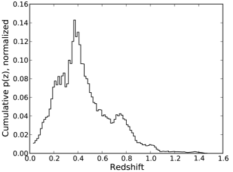
Figure 28: Cumulative $p(z)$ of all SDSS galaxies, based on DR7 $p(z)$ (Cunha et al., 2009). Although in the $p(z)$ method, the calibration samples are weighted to better represent the whole of the SDSS photometric sample, the LSS evident in the calibration set appears in the $p(z)$ photometric redshifts (cf. fig. 17 of Cunha et al. 2009 for the training set distribution). The excess at $z\sim 0.75$ is due to the non-EGS DEEP2 spectroscopic training subsample, which intentionally targets high-$z$ objects. (The split at $z\sim 0.3$ is due to an issue in the training set, and is absent in the DR8 version of the $p(z)$; Sheldon et al. 2011 in prep.)

The cc2 and d1 neural net methods, as well as the $p(z)$ redshift probability distribution, also use the SDSS MAIN (435k) and LRG ($>$80k) spectroscopic samples as the training set, with supplements from other spectroscopic samples with deeper flux limits and broader redshift coverage, but smaller size ($\sim 7$k). For the $p(z)$ method, the training samples are then weighted to reproduce the $r$-magnitude and color distributions of the photometric sample. The limited number of high-$z$ regions contributing to photo-$z$ estimation results in the LSS in those regions being imprinted onto the output photo-$z$ for the full photometric sample (see Fig. 28). The excess at $z\sim 0.75$ is due mostly to the non-EGS DEEP2 spectroscopic training subsample, because they select high-$z$ ($z\gtrsim 0.7$) galaxies to target. Since the DEEP2 targeting were based on non-SDSS bands, the magnitude-based reweighting scheme is not complete, causing the excess structure. Additionally, any LSS present in the training set reflects directly into the $p(z)$ (Sheldon et al. 2011, in prep.). In general, if the sample we use to test our calibration is also in the training set (which is the case here), then we expect excessively optimistic results. There are simply not enough spectroscopic samples at high-$z$ available to split between testing and training.

For the lens sample, in addition to aiming for photo-$z$ accuracy, we require $k$-correction for our galaxy-galaxy lensing analysis, to stack lenses according to $k$-corrected galaxy observables such as luminosity and colour. Such information is not available with the d1 and cc2 methods, despite having the least bias and scatter for the lens sample. Although training-set based method can, in principle, perform spectral classifications (Firth et al., 2003; Collister & Lahav, 2004), the estimated SED it is not available with these photo-$z$’s, and hence $k$-correction is not available. The hybrid method includes an SED estimator which enables a $k$-correction, but their $z_{\rm phot}$ scatter at low photo-$z$ is higher than with the ZEBRA method.

We briefly compare our photo-$z$ to the MegaZ-LRG sample by Collister et al. (2007) with a scatter of $\sigma_{\Delta z/(1+z)}=0.045$. We impose the MegaZ-LRG color and magnitude cuts to our calibration sample, and find that ZEBRA classifies the calibration sample into Ell and Sbc types with 259 and 102 objects, with scatter of $\sigma_{\Delta z/(1+z)}=0.04$ and 0.07, respectively. For the combined sample, the scatter is 0.05. While the scatter in our calibration sample is not quite as small as that from MegaZ-LRG, our cuts do not include the fiber magnitude cut or the magnitude-based star-galaxy separation criteria cuts imposed on the MegaZ-LRG sample, which presumably would decrease the number of outliers we see in our photo-$z$ error. Additionally, we note that our need for $k$-corrections to define luminosities prevents us from using photo-z estimators without any template information, such as the neural net method of Collister et al. (2007).

References

- Abazajian et al. (2009) Abazajian K. N., et al. 2009, Astrophys. J. Supp., 182, 543
- Abdalla et al. (2008) Abdalla F. B., Banerji M., Lahav O., Rashkov V., 2008, preprint (arXiv:0812.3831)
- Albrecht et al. (2006) Albrecht A., et al. 2006, preprint (arXiv:0609591)
- Baldauf et al. (2010) Baldauf T., Smith R. E., Seljak U., Mandelbaum R., 2010, Phys. Rev. D, 81, 063531
- Bartelmann & Schneider (2001) Bartelmann M., Schneider P., 2001, Phys. Rep., 340, 291
- Bell et al. (2003) Bell E. F., McIntosh D. H., Katz N., Weinberg M. D., 2003, Astrophys. J. Supp., 149, 289
- Benítez (2000) Benítez N., 2000, Astrophys. J., 536, 571
- Blanton & Roweis (2007) Blanton M. R., Roweis S., 2007, Astron. J., 133, 734
- Brown et al. (2007) Brown M. J. I., et al. 2007, Astrophys. J., 654, 858
- Bruzual & Charlot (2003) Bruzual G., Charlot S., 2003, Mon. Not. R. Astron. Soc., 344, 1000
- Bruzual & Charlot (1993) Bruzual A. G., Charlot S., 1993, Astrophys. J., 405, 538
- Budavári et al. (2000) Budavári T., Szalay A. S., Connolly A. J., Csabai I., Dickinson M., 2000, Astron. J., 120, 1588
- Cacciato et al. (2009) Cacciato M., van den Bosch F. C., More S., Li R., Mo H. J., Yang X., 2009, Mon. Not. R. Astron. Soc., 394, 929
- Capak et al. (2007) Capak P., et al. 2007, Astrophys. J. Supp., 172, 99
- Coil et al. (2010) Coil A. L., et al. 2010, preprint (arXiv:1011.4307)
- Coil et al. (2004) Coil A. L., et al. 2004, Astrophys. J., 609, 525
- Coleman et al. (1980) Coleman G. D., Wu C., Weedman D. W., 1980, Astrophys. J. Supp., 43, 393
- Collister et al. (2007) Collister A., et al. 2007, Mon. Not. R. Astron. Soc., 375, 68
- Collister & Lahav (2004) Collister A. A., Lahav O., 2004, Pub. Astron. Soc. Pacific, 116, 345
- Csabai et al. (2003) Csabai I., et al. 2003, Astron. J., 125, 580
- Cunha et al. (2009) Cunha C. E., Lima M., Oyaizu H., Frieman J., Lin H., 2009, Mon. Not. R. Astron. Soc., 396, 2379
- Davis et al. (2003) Davis M., et al. 2003, in P. Guhathakurta ed., Proc. SPIE Vol. 4834, Discoveries and Research Prospects from 6- and 10-Meter-Class Telescopes II. SPIE, Bellingham, p. 161
- Davis et al. (2005) Davis M., Gerke B. F., Newman J. A., 2005, in Wolff S. C., Lauer T. R., eds, ASP Conf. Ser. Vol. 339, Observing Dark Energy. Astronom. Soc. Pac., San Francisco, p. 269 p. 128
- Davis et al. (2007) Davis M., et al. 2007, Astrophys. J. Lett., 660, L1
- Dutton et al. (2010) Dutton A. A., et al. 2010, preprint (arXiv:1012.5859)
- Eisenstein et al. (2001) Eisenstein D. J., et al. 2001, Astron. J., 122, 2267
- Eisenstein et al. (2011) Eisenstein D. J., et al. 2011, preprint (arXiv:1101.1529)
- Faber et al. (2003) Faber S. M., et al. 2003, in Iye M., Moorwood A. F. M., eds, Proc. SPIE Vol. 4841, Instrument Design and Performance for Optical/Infrared Ground-based Telescopes. SPIE, Bellingham, p. 1657
- Faber et al. (2007) Faber S. M., et al. 2007, Astrophys. J., 665, 265
- Feldmann et al. (2006) Feldmann R., et al. 2006, Mon. Not. R. Astron. Soc., 372, 565
- Firth et al. (2003) Firth A. E., Lahav O., Somerville R. S., 2003, Mon. Not. R. Astron. Soc., 339, 1195
- Fu et al. (2008) Fu L., et al. 2008, Astron. Astrophys., 479, 9
- Fukugita et al. (1996) Fukugita M., Ichikawa T., Gunn J. E., Doi M., Shimasaku K., Schneider D. P., 1996, Astron. J., 111, 1748
- Giallongo et al. (2005) Giallongo E., et al. 2005, Astrophys. J., 622, 116
- Gunn et al. (1998) Gunn J. E., et al. 1998, Astron. J., 116, 3040
- Heymans et al. (2006) Heymans C., et al. 2006, Mon. Not. R. Astron. Soc., 371, L60
- Hildebrandt et al. (2010) Hildebrandt H., et al. 2010, Astron. Astrophys., 523, A31
- Hirata & Seljak (2003) Hirata C., Seljak U., 2003, Mon. Not. R. Astron. Soc., 343, 459
- Hoekstra et al. (2005) Hoekstra H., Hsieh B. C., Yee H. K. C., Lin H., Gladders M. D., 2005, Astrophys. J., 635, 73
- Hogg et al. (2002) Hogg D. W., Baldry I. K., Blanton M. R., Eisenstein D. J., 2002, preprint (arXiv:0210394)
- Hogg et al. (2001) Hogg D. W., Finkbeiner D. P., Schlegel D. J., Gunn J. E., 2001, Astron. J., 122, 2129
- Ilbert et al. (2006) Ilbert O., et al. 2006, Astron. Astrophys., 457, 841
- Ilbert et al. (2009) Ilbert O., et al. 2009, Astrophys. J., 690, 1236
- Ivezić et al. (2004) Ivezić Ž., et al. 2004, Astronomische Nachrichten, 325, 583
- Kinney et al. (1996) Kinney A. L., et al. 1996, Astrophys. J., 467, 38
- Kleinheinrich et al. (2005) Kleinheinrich M., et al. 2005, Astron. Astrophys., 439, 513
- Kleinheinrich et al. (2006) Kleinheinrich M., et al. 2006, Astron. Astrophys., 455, 441
- Komatsu et al. (2011) Komatsu E., et al. 2011, Astrophys. J. Supp., 192, 18
- Le Fèvre et al. (2005) Le Fèvre O., et al. 2005, Astron. Astrophys., 439, 845
- Leauthaud et al. (2011) Leauthaud A., et al. 2011, preprint (arXiv:1104.0928)
- LeFevre et al. (2003) LeFevre O., et al. 2003, in Iye M., Moorwood A. F. M., eds, Proc. SPIE, Vol. 4841, Instrument Design and Performance for Optical/Infrared Ground-based Telescopes. SPIE, Bellingham, p. 1670
- Lilly et al. (2009) Lilly S. J., et al. 2009, Astrophys. J. Supp., 184, 218
- Lilly et al. (2007) Lilly S. J., et al. 2007, Astrophys. J. Supp., 172, 70
- Lupton et al. (2001) Lupton R., et al. 2001, in F. R. Harnden Jr., F. A. Primini, & H. E. Payne ed., ASP Conf. Ser. Vol. 238, Astronomical Data Analysis Software and Systems X. Astronom. Soc. Pac., San Francisco, p. 269
- Madau (1995) Madau P., 1995, Astrophys. J., 441, 18
- Madgwick et al. (2003) Madgwick D. S., et al. 2003, Astrophys. J., 599, 997
- Mandelbaum et al. (2005) Mandelbaum R., et al. 2005, Mon. Not. R. Astron. Soc., 361, 1287
- Mandelbaum et al. (2009) Mandelbaum R., Li C., Kauffmann G., White S. D. M., 2009, Mon. Not. R. Astron. Soc., 393, 377
- Mandelbaum et al. (2010) Mandelbaum R., Seljak U., Baldauf T., Smith R. E., 2010, Mon. Not. R. Astron. Soc., 405, 2078
- Mandelbaum et al. (2008) Mandelbaum R., Seljak U., Hirata C. M., 2008, JCAP , 8, 6
- Mandelbaum et al. (2008) Mandelbaum R., et al. 2008, Mon. Not. R. Astron. Soc., 386, 781
- Mandelbaum et al. (2006) Mandelbaum R., Seljak U., Kauffmann G., Hirata C. M., Brinkmann J., 2006, Mon. Not. R. Astron. Soc., 368, 715
- Meiksin (2006) Meiksin A., 2006, Mon. Not. R. Astron. Soc., 365, 807
- Oguri & Takada (2011) Oguri M., Takada M., 2011, Phys. Rev. D, 83, 023008
- Oyaizu et al. (2008) Oyaizu H., Lima M., Cunha C. E., Lin H., Frieman J., Sheldon E. S., 2008, Astrophys. J., 674, 768
- Padmanabhan et al. (2008) Padmanabhan N., et al. 2008, Astrophys. J., 674, 1217
- Parker et al. (2007) Parker L. C., Hoekstra H., Hudson M. J., van Waerbeke L., Mellier Y., 2007, Astrophys. J., 669, 21
- Pier et al. (2003) Pier J. R., et al. 2003, Astron. J., 125, 1559
- Refregier (2003) Refregier A., 2003, Annu. Rev. Astron. Astrophys., 41, 645
- Reyes et al. (2008) Reyes R., Mandelbaum R., Hirata C., Bahcall N., Seljak U., 2008, Mon. Not. R. Astron. Soc., 390, 1157
- Reyes et al. (2010) Reyes R., Mandelbaum R., Seljak U., Baldauf T., Gunn J. E., Lombriser L., Smith R. E., 2010, Nature, 464, 256
- Richards et al. (2002) Richards G. T., et al. 2002, Astron. J., 123, 2945
- Schlegel et al. (1998) Schlegel D. J., Finkbeiner D. P., Davis M., 1998, Astrophys. J., 500, 525
- Schrabback et al. (2010) Schrabback T., et al. 2010, Astron. Astrophys., 516, A63
- Schulz et al. (2010) Schulz A. E., Mandelbaum R., Padmanabhan N., 2010, Mon. Not. R. Astron. Soc., 408, 1463
- Scoville et al. (2007a) Scoville N., et al. 2007a, Astrophys. J. Supp., 172, 1
- Scoville et al. (2007b) Scoville N., et al. 2007b, Astrophys. J. Supp., 172, 38
- Sheldon et al. (2004) Sheldon E. S., et al. 2004, Astron. J., 127, 2544
- Sheldon et al. (2009) Sheldon E. S., et al. 2009, Astrophys. J., 703, 2217
- Smith et al. (2002) Smith J. A., et al. 2002, Astron. J., 123, 2121
- Stoughton et al. (2002) Stoughton C., et al. 2002, Astron. J., 123, 485
- Stoughton et al. (2002) Stoughton C., et al. 2002, Astron. J., 123, 485
- Strauss et al. (2002) Strauss M. A., et al. 2002, Astron. J., 124, 1810
- Taniguchi et al. (2007) Taniguchi Y., et al. 2007, Astrophys. J. Supp., 172, 9
- Tucker et al. (2006) Tucker D. L., et al. 2006, Astronomische Nachrichten, 327, 821
- Willmer et al. (2006) Willmer C. N. A., et al. 2006, Astrophys. J., 647, 853
- Wolf et al. (2003) Wolf C., Meisenheimer K., Rix H.-W., Borch A., Dye S., Kleinheinrich M., 2003, Astron. Astrophys., 401, 73
- Yoo et al. (2006) Yoo J., Tinker J. L., Weinberg D. H., Zheng Z., Katz N., Davé R., 2006, Astrophys. J., 652, 26
- York et al. (2000) York D. G., et al. 2000, Astron. J., 120, 1579
- Zhang et al. (2007) Zhang P., Liguori M., Bean R., Dodelson S., 2007, Physical Review Letters, 99, 141302