A fast Monte Carlo algorithm for studying bottle-brush polymers
Abstract
Obtaining reliable estimates of the statistical properties of complex macromolecules by computer simulation is a task that requires high computational effort as well as the development of highly efficient simulation algorithms. We present here an algorithm combining local moves, the pivot algorithm, and an adjustable simulation lattice box for simulating dilute systems of bottle-brush polymers with a flexible backbone and flexible side chains under good solvent conditions. Applying this algorithm to the bond fluctuation model, very precise estimates of the mean square end-to-end distances and gyration radii of the backbone and side chains are obtained, and the conformational properties of such a complex macromolecule are studied. Varying the backbone length (from to ), side chain length (from to or ), the scaling predictions for the backbone behavior as well as the side chain behavior are checked. We are also able to give a direct comparison of the structure factor between experimental data and the simulation results.
I Introduction
The so-called “bottle-brush polymers” consist of a long macromolecule serving as a “backbone” on which many flexible side chains are densely grafted Zhang2005 ; Subbotin2007 ; Sheiko2008 ; Potemkin2009 . In nature, bottle-brush like aggrecans have been found in the cartilage of mammalian including human joints and are indeed held responsible for the excellent lubrication properties in such joints Klein2006 ; Klein2009 . Recently, the chemical synthesis of such complex molecular bottle-brushes has become possible in laboratories with newly developed synthetic techniques Wintermantel1994 ; Wintermantel1996 ; Rathgeber2005 ; Zhang2006 . Theoretical predictions [11-42] of the conformational properties of bottle-brush polymers based on the blob picture, the scaling theory, and the self-consistent field theory have also been worked out. However, in order to check the theoretical predictions and to give a reasonable explanation for the experimental results or to control the functions of bottle-brush polymers computer simulations are needed for a deeper understanding of the structure of these macromolecules.
“Static” Monte Carlo (MC) algorithms (simple sampling of self-avoiding walks (SAWs)), extensions such as dimerization, enrichment techniques, Rosenbluth’s inversely restricted sampling and the pruned enriched Rosenbluth method (PERM) do not converge for very large branched polymers such as bottle-brushes. “Dynamic” MC algorithms also encounter serious problems, since the relaxation times of these polymers are expected to be excessively large, and hence prohibitively long MC simulations would be required. In the early work on bottle-brush polymers in a good solvent, both lattice and off-lattice models were used for MC simulations. Using the bond fluctuation model Carmesin1988 ; Deutsch1991 ; Paul1991 ; Binder1995 on a simple cubic lattice, applying local moves to the bottle-brush polymers, side chain lengths up to , backbone lengths up to , and grafting densities up to were studied in Shiokawa1999 . In combination with the pivot move algorithm, up to , up to , and were studied in Rouault1996 ; Rouault1998 . Using flexible freely jointed chains Saariaho1997 ; Yethiraj2006 and the bead-spring model Elli2004 with hard sphere interactions in a continuous space and using the pivot moves, the largest bottle-brush polymers which were studied were , , and , and using the Metropolis algorithm for the latter model, maximum values of , were studied. However, although all these studies clearly are very interesting and stimulating, the accessible parameter range clearly was not large enough (and the accuracy of the results not precise enough) to allow a straightforward test of the theoretical concepts, and thus a need for further work with different methods clearly did emerge.
In our previous work Hsu2007a ; Hsu2007b , we were able to simulate bottle-brush polymers with rigid linear backbone and flexible side chains under various solvent conditions by applying a variant of the PERM algorithm Grassberger1997 to a simple lattice model with periodic boundary conditions along the backbone. Under good solvent conditions, we have shown that the power laws predicted for the side chain behavior are still difficult to reach although the maximum side chain length in our simulation was . However, a crossover behavior from 3D SAW-like side chains to stretched side chains was presented in Hsu2007a ; Hsu2007b as the side chain length or the grafting density increased. Of course, removing all configurational degrees of freedom of the backbone was a crucial prerequisite to allow the successful use of the PERM algorithm, but it also means that highly interesting questions (such as backbone stiffening due to the side chains) could not be studied.
Recently, we have focused on the comparison of structure factors to experimental data and on the persistence length Hsu2009 ; Hsu2010a ; Hsu2010b of the backbone using the bond fluctuation model on a simple cubic lattice. This communication will discuss in detail the algorithm we developed for these simulations. It is introduced in Sec. II, and results for the conformational properties of bottle-brush polymers only achievable by this very efficient simulation approach are shown in Sec. III. Finally, our conclusions are presented in Sec. IV.

II Model and Simulation methods
For studying bottle-brush polymers with a flexible backbone and with flexible side chains under very good solvent conditions so that only excluded volume effects are considered, we generalize the standard bond fluctuation model for linear polymers Carmesin1988 ; Deutsch1991 ; Paul1991 ; Binder1995 to bottle-brush polymers. In the standard bond fluctuation model, a flexible polymer chain with excluded volume interactions is described by a chain of effective monomers on a simple cubic lattice (the lattice spacing is the unit of length). Each effective monomer blocks all 8 corners of an elementary cube of the lattice from further occupation. Two successive monomers along a chain are connected by a bond vector which is taken from the set , , , , , , including also all permutations. The bond length is in a range between and . There are in total 108 bond vectors serving as candidates for building the conformational structure of bottle-brush polymers.
(a)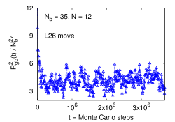 (b)
(b)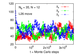
As shown in Fig. 1, the geometry of the bottle-brush polymer is arranged in a way that side chains of length are added to the backbone at a regular spacing ( is the grafting density), and two additional monomers are added to the two ends of the backbone. Thus, the number of monomers of the backbone is related to the number of side chains via
| (1) |
and the total number of monomers of the bottle-brush polymer is . Creating an initial configuration of a bottle-brush polymer that does not violate any excluded volume constraint would be a highly nontrivial matter if we would require that both backbone and side chains are already coiled. Thus one simple way to construct an initial configuration of bottle-brush polymers in the simulation is to assume that the backbone and all side chains are rigid rod-like structures. In order to fit the criteria of the bond fluctuation model without further checking, the backbone is placed in the direction along the -axis with fixed bond length between two successive monomers on the backbone. The bond vectors of each side chain are chosen randomly from one of the allowed bond vectors in the ()-plane, but the bond vectors used to connect the monomers on the same side chain starting from the grafting site on the backbone are the same.
In our algorithm, instead of trying to move a monomer to the nearest neighbor sites in the six directions (“L6” move), , , and for the standard bond fluctuation model, we use the local 26 (“L26”) moves Wittmer2007 . Namely, the chosen monomer is allowed to move to not only the nearest neighbor sites but also the next neighbor sites, and the sites at the 8 corners, which are located , and lattice spacings away from the chosen monomer, respectively. The move is accepted only if the selected new positions are empty and the bond length constraints are satisfied. The key point of this move is that it allows for crossings of bonds during the move; no such simple moves that allow bond crossing for the simple SAW model (where the bond length is fixed to one lattice spacing) are known. Without the possibility of bond crossing, two side chains of the bottle-brush that happen to be entangled with each other would relax this topological constraint only extremely slowly.
(a)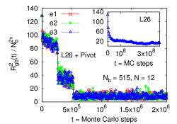 (b)
(b)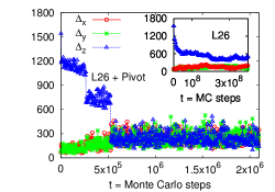
Since neighboring side chains are rigidly grafted to neighboring “anchor points” at the backbone, they can never diffuse away from each other, unlike free chains in a solution or melt; thus topological constraints could relax only via an “arm retraction mechanism” familiar from star polymers, if the algorithm ensures non-crossability of chains. This arm reaction leads to an extremely long relaxation time. This problem is avoided by the “L26” moves. Applying the “L26” move algorithm to a small bottle-brush polymer of 431 monomers (, , and ), results of the time series of the square gyration radius of the backbone scaled with the scaling law for 3D SAWs, (), and the time series of the shape change of bottle-brush polymers, which is described by the space occupation in the Cartesian coordinates shown in Fig. 2 indicate that it needs about MC steps to reach an equilibrium state. Here one MC step is a sequence of “L26” moves (each monomer is attempted to move once). As the number of monomers on the backbone increases to , i.e., the total number of monomers increases to , one would expect for a Rouse scaling of the relaxation time that it might need about times the number of MC steps to reach an equilibrium state. Unfortunately, the simple Rouse behavior does not describe the scaling of the relaxation time for the bottle-brushes and the relaxation time increases even faster as shown in the inset of Fig. 3.
(a)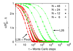 (b)
(b)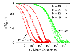
In our simulations, the lattice size is chosen large enough so that no monomer can interact with itself. The th monomer located at the site is denoted by . No periodic boundary condition is considered here but a hashing method is used to map the position of monomers back into the original box. For small bottle-brush polymers it is possible to set the lengths of the simple cubic lattice equal in each dimension, i.e., (the maximum length determined by the initial configuration), while for large bottle-brush polymers one encounters difficulties in the limitation of computer memory. Therefore, in order to be able to simulate large bottle-brush polymers, a new method is introduced which separates the equilibrating process into several stages. The maximum lattice size which we can use on the computer is . Thus, we first choose , , and . As shown in Fig. 3, the time series of , , and as well as configurations in the intermediate state are stored. After MC steps, we reset the size of the lattice by decreasing to but increasing and to . Here is the number of MC steps at the current stage, which can be adopted to the simulation such that the condition and holds. We repeat the same procedure until since the space occupation of the conformations of bottle-brush polymers must be isotropic.
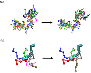
To speed up the equilibrating process and the time for generating independent configurations, in addition to the local “L26” move Wittmer2007 also pivot moves Sokal1995 are used. Two types of moves are attempted (see Fig 4):
-
(i)
a monomer on the backbone is chosen randomly and the short part of the bottle-brush polymer is transformed by randomly applying one of the 48 symmetry operations (no change; rotations by 90o and 180o; reflections and inversions) to the adjacent bond.
-
(ii)
A monomer is chosen randomly from all the side chain monomers, and the part of the side chain from the selected monomer to the free end of the side chain is transformed by one of the 48 symmetry operations.
Again, we apply the “L26 + pivot” algorithm to the bottle-brush polymers with , , and but start the simulations from three different initial configurations named by e1, e2, and e3. From the results shown in Fig. 3, we see that the equilibrium states are reached in less than MC steps. Here one MC step is a sequence of “L26” moves, pivot moves of the backbone and pivot moves of side chains; is chosen such that the acceptance ratio is about or even larger, while . It takes about 1.25 hours CPU time on an Intel 2.80 GHz PC to reach the equilibrium state (after MC steps are performed) for one single simulation of bottle-brush polymers (, , and ) with , , and .
Another important point one has to be aware of is that the monomers on the backbone, labelled as , , , , which can be selected as a pivot point for applying the pivot move are also limited due to the size of the lattice we set up before reaching the equilibrium state. However, once the system is in equilibrium one has to allow all possible moves () with the “L26+pivot” algorithm. For the case shown in Fig. 3, the equilibrating process is divided into four stages:
(a)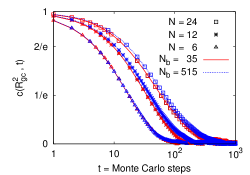 (b)
(b)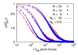
- stage 1:
-
, , , MC steps
- stage 2:
-
, , , MC steps
- stage 3:
-
, , , MC steps
- stage 4:
-
, , MC steps
As a caveat, the number of stages needed for the system reaching the equilibrium is empirical. It varies according to the size of the backbone length and fluctuations from one equilibration path to the other equilibration path. When one simulates an end-grafted bottle-brush polymer adsorbed to an impenetrable flat surface, it also varies depending on the attractive interactions between the monomers and the surface. Due to the fluctuation of the conformations of bottle-brush polymers, the time series of the square gyration radius of the backbone, , and the space occupations in the Cartesian coordinations of the bottle-brush polymers (similar to the functions shown in Fig. 3) are required in order to determine the lengths of the simulation box for the next stage and to check whether the equilibrating process is finished or not.
The efficiency of the algorithm and the number of MC steps needed for getting an independent configuration for the measurement were determined by the autocorrelation function ,
| (2) |
where is an observable. Results of for the mean square gyration radius of the backbone, , and of the side chains, (taking the average of all side chains at the same Monte Carlo time ) plotted against the number of MC steps are shown in Fig. 5 for . We see that the “L26+pivot” algorithm is two orders of magnitude faster than the “L26” algorithm for the four cases of bottle-brush polymers (backbone length , grafting density , and side chain lengths , , , and ) we chose. Also, increasing the side chain length from to , the autocorrelation time for the side chain structural relaxation increases by more than two orders of magnitude for the “L26” case and by less than one order of magnitude for the “L26+pivot” case. When we increase the backbone length to and adjust the number of pivot moves for the side chains tried from to in each Monte Carlo step such that on average about of the side chains is tried for a pivot move in each MC step, we can see in part a) of Fig. 6 that the decay of the autocorrelation function for the side chain structure occurs on the same time scale, i.e., it is only the average number of pivot moves per side chain which determines the autocorrelation time. The same is true for the backbone as we can see in part b) of that figure. Here we plot the autocorrelation function explicitly against the total number of pivot moves tried, , and it is obvious that the structural relaxation for the much longer backbone chain occurs on the same time scale as the one for the short backbone chain. A systematic increase of the relaxation time for both, side chains and backbone, as a function of side chain length remains, however. The stage wise decomposition of the equilibrating process, with the appropriate adjustment of the simulation volume, as described above, is a crucial step of our procedures, and a novel ingredient, not used in other contexts, and was a prerequisite for successful simulations.
(a)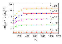 (b)
(b)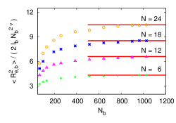
III Results
In order to test our program, we first simulated linear polymer chains of monomers under good solvent conditions, i.e., . According to the scaling law of the mean square end-to-end distance, , one should expect that the curve of becomes horizontal as . Here is the Flory exponent for the 3D SAW. This is indeed seen in Fig. 7. Using the “L26+pivot” algorithm, we can simulate bottle-brush polymers with a number of monomers on the backbone up to , side chain length up to for , and side chain length up to for . The results shown in Fig. 7 are the average of - independent configurations. The error bars are given by the standard deviations of the average, which are smaller than the size of symbols. Increasing the side chain length , but keeping the grafting density fixed to or , one observes an increase in for a fixed value of , which shows that the stretching of the backbone is induced by the chain length as well as the grafting density , whereas one observes that the backbone of the bottle-brush polymers behaves like a SAW with increasing but fixed . In Ref. Hsu2010a ; Hsu2010b , it has been pointed out that the persistence length which describes the intrinsic stiffness of bottle-brush polymers can be determined by the mean square end-to-end distance of the backbone, ,
| (3) |
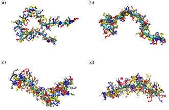
Here is the average bond length of polymer chains for the bond fluctuation model. The snapshots of conformations of bottle-brush polymers which contain monomers on the backbone and monomers on each side chain in a good solvent displayed in Fig. 8 also show that the backbone becomes stiffer as the side chain length increases from to .
(a)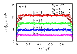 (b)
(b)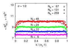
Another quantity which can be used to examine whether the system does reach the equilibrium and the statistics are reliable enough is the mean square end-to-end distance (or radius of gyration ) of the side chains along the backbone in the direction perpendicular to the backbone. For bottle-brush polymers of a flexible backbone, the perpendicular direction is determined by the vector pointing from the grafting site to the center of mass of the corresponding grafted side chain. Plotting against the normalized position for , , , in Fig. 9, a plateau appears with tiny fluctuations for showing that in the interior of bottle-brush polymers the side chains behave the same for fixed side chain lengths as expected after taking the average over sufficiently many independent samples. The side chains stretch away more from the backbone as the side chain length and the grafting density increases. The decreasing behavior of for the side chains near the two ends of the backbone obviously arises from the fact that monomers on these side chains have more freedom to move.
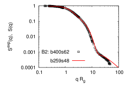
Finally, a comparison of the structure factor between the experimental data Rathgeber2005 and our simulation results Hsu2010a is shown in Fig. 10. The normalized structure factor is defined by
| (4) |
where is an occupation variable, if the site is occupied by a bead, and zero otherwise. Note that an angular average over the direction of the scattering vector has been performed, and the sums run over all monomers (all side chains and the backbone). Adjusting only the number of monomers on the backbone, , and the number of monomers on each side chain, , the results for the bottle-brush polymers of , , and are mapped to the data for the experimental sample of , and when the momentum is scaled by . Here is the gyration radius of the whole bottle-brush polymer. In this case, (lattice spacings) is obtained from our MC simulations and nm is obtained from the experimental data. One can immediately translate nm lattice spacing. Clearly, translating the length units from the large-scale structure (small behavior) and choosing the length of backbone and side chains correctly, one obtains a faithful description of the experimental scattering function over the whole -range studied.
IV Conclusion
We have presented extensive MC simulations for bottle-brush polymers under good solvent conditions using the bond fluctuation model with a newly developed efficient MC algorithm combining the “L26” moves, the pivot moves, and an adjustable simulation lattice box which changes its shape from a very elongated parallelepiped to a cube as the equilibration of the bottle-brush polymer conformation from an initial stretched backbone to a coiled conformation proceeds. Using this fast algorithm to generate a sufficiently large number of independent configurations in equilibrium, we are able to obtain high accuracy estimates of the related characteristic length scales for describing the conformational properties of bottle-brush polymers, such as the end-to-end distance of a side chain and the backbone, the persistence length of the backbone, the effective cross-sectional radius of the whole bottle-brush polymers etc. From the computer simulations, the scattering intensity contributed by any part of the bottle-brush polymers are calculated directly. Therefore, we are also able to compare our simulation result to the experimental data directly and test those models used in the analysis of experimental data.
Recently, this algorithm has also been employed successfully to study the conformational change of bottle-brush polymers as they are absorbed on a flat solid surface by varying the attractive interaction between the monomers and the surface Hsu2010c . In our future work, it will be interesting to see how far this algorithm can be applied for studying bottle-brush polymers under poorer solvent conditions.
V Acknowledgments
H.-P. H. received funding from the Deutsche Forschungsgemeinschaft (DFG), grant No SFB 625/A3. We are grateful for extensive grants of computer time at the JUROPA under the project No HMZ03 and SOFTCOMP computers at the Jülich Supercomputing Centre (JSC). H.-P. H. thanks J. Baschnagel, H. Meyer, and J. P. Wittmer for stimulating discussions during her visit at the Institut Charles Sadron, Strasbourg, France. We also thank K. Binder for very useful discussions and for critically reading the manuscript.
References
- (1) M. Zhang, A.H.E. Müller, Cylindrical Polymr Brushes, J. Polym. Sci, Part A, Polymer Chemistry 43 (2005) 3461-3481.
- (2) A. V. Subbotin, A. N. Semenov, Spatial self-organization of comb macromolecules, Polym. Sci. Ser. A 49 (2007) 1328-1357.
- (3) S. S. Sheiko, B. S. Sumerlin, K. Matyjaszewski, Cylindrical molecular brushes: Synthesis, characterization, and properties, Prog. Polym. Sci. 33 (2008) 759-785.
- (4) I. I. Potemkin, V. V. Palyulin, Comblike macromolecules, Prog. Polym. Sci. 51 (2009) 123-149.
- (5) J. Klein, Molecular mechanisms of synovial joint lubrication Proc. Inst. Mech. Eng. Part J 220 (2006) 691-710.
- (6) J. Klein, Repair or replacement - A joint perspective, Science 323 (2009) 47-48.
- (7) M. Wintermantel, M. Schmidt, Y, Tsukaharam, K. Kajiwara, S. Kohjiya, Rodlike combs, Macromol. Chem. Rapid Commun. 15 (1994) 279-284.
- (8) M. Wintermantel, M. Gerle, K. Fischer, M. Schmidt, I. Wataoka, H. Urakawa, K. Kajiwara, Y. Tsukahara, Molecular Bottlebrushes, Macromolecules 29 (1996) 978-983.
- (9) S. Rathgeber, T. Pakula, K. Matyjaszewski, K. L. Beers, On the shape of bottle-brush macromolecules: Systematic variation of architectural parameters, J. Chem. Phys. 122 (2005) 124904-1-124904-13.
- (10) B. Zhang, F. Gröhn, J. S. Pedersen, K. Fischer, M. Schmidt, Conformation of cylindrical brushes in solution: Effect of side chain length, Macromolecules 39 (2006) 8440.
- (11) T. M. Birshtein, E. B. Zhulina, Conformations of star-branched macromolecules, Polymer 25 (1984) 1453-1461.
- (12) T. A. Witten, P. A. Pincus, Colloid stabilization by long grafted polymers, Macromolecules 19 (1986) 2509-2513.
- (13) T. M. Birshtein, O. V. Borisov, Ye. B. Zhulina, A. R. Khokhlov, T. A. Yurasova, Conformations of comb-like macromolecules, Polym. Sci. USSR 29 (1987) 1293-1300.
- (14) Z.-G. Wang, S. A. Safran, Size distribution for aggregates of associating polymers. II. Linear packing, J. Chem. Phys. 89 (1988) 5323-5328.
- (15) C. Ligoure, L. Leibler, Decoration of rough surfaces by chain grafting, Macromolecules 23 (1990) 5044-5046.
- (16) R. C. Ball, J. F. Marko, S. T., Milner, T. A. Witten, Polymers grafted to a convex surface, Macromolecules 24 (1991) 693-703.
- (17) M. Murat, G. S. Grest, Polymers end-grafted onto a cylindrical surface, Macromolecules 24 (1991) 704-708.
- (18) N. Dan, M. Tirrell, Polymers tethered to curved interfaces. A self-consistent-field analysis, Macromolecules 25 (1992) 2890-2895.
- (19) G. H. Fredrickson, Surfactant-induced lyotropic behavior of flexible polymer solutions, Macromolecules 26 (1993) 2825-2831.
- (20) E. B. Zhulina, T. A. Vilgis, Scaling theory of planar brushes formed by branched polymers, Macromolecules 28 (1995) 1008-1015.
- (21) E. M. Sevick, Shear swelling of polymer brushes grafted onto convex and concave surface, Macromolecules 29 (1996) 6952-6958.
- (22) Y. Rouault, O. V. Borisov, Comb-Branched polymers: Monte Carlo simulation and scaling, Macromolecules 29 (1996) 2605-2611.
- (23) M. Saariaho, O. Ikkala, I. Szleifer, I. Erukhimovich, G. ten Brinke, On lyotropic behavior of molecular bottle-brushes: A Monte Carlo computer simulation study, J. Chem. Phys. 107 (1997) 3267-3276.
- (24) M. Saariaho, I. Szleifer, O. Ikkala, O. G. ten Brinke, Extended conformations of isolated molecular bottle-brushes: Influence of side-chain topology, Macromol. Theory Simul. 7 (1998) 211-216.
- (25) Y. Rouault, From comb polymers to polysoaps: A Monte Carlo attempt, Macromol. Theory Simul. 7 (1998) 359-365.
- (26) K. Shiokawa, K. Itoh, N. Nemoto, Simulations of the shape of a regularly branched polymer as a model of a polymacromonomer, J. Chem. Phys. 111 (1999) 8165-8173.
- (27) M. Saariaho, A. Subbotin, I. Szleifer, O. Ikkala, G. ten Brinke, Effect of side chain rigidity on the elasticity of comb copolymer cylindrical brushes: A Monte Carlo simulation study, Macromolecules 32 (1999) 4439-4443.
- (28) A. Subbotin, M. Saariaho, O. Ikkala, G. ten Brinke, Elasticity of comb copolymer cylindrical brushes, Macromolecules 33 (2000) 3447-3452.
- (29) M. Saariaho, A. Subbotin, O. Ikkala, G. ten Brinke, Comb copolymer cylindrical brushes containing semiflexible side chains: a Monte Carlo study, Macromol.Rapid. Commun. 21 (2000) 110-115.
- (30) P. G. Khalatur, D. G. Shirvanyanz, N. Y. Starovoitova, A. R. Khokhlov, Conformational properties and dynamics of molecular bottle-brushes: A cellular-automaton-based simulation, Macromol. Theory Simul. 9 (2000) 141-155.
- (31) V. V. Vasilevskaya, A. A. Klochkov, P. G. Khalatur, A. R. Khokhlov, G. ten Brinke, Microphase separation within a comb copolymer with attractive side chains: A computer simulation study. Macromol. Theory Simul. 10 (2001) 389-394.
- (32) A. Yethiraj, A Monte Carlo simulation study of branched polymers, J. Chem. Phys. 125 (2006) 204901 10 pages.
- (33) N. A. Denesyuk, Conformational properties of bottle-brush polymers, Phys. Rev. E 67 (2003) 051803 10 pages.
- (34) S. S. Sheiko, O. V. Borisov, S. A. Prokhorova, M. Möller, Cylindrical molecular brushes under poor solvent conditions: microscopic observation and scaling analysis, Eur. Phys. J. E 13 (2004) 125-131.
- (35) S. Elli, F. Ganazzoli, E. G. Timoshenko, Y. A. Kuznetsov, R. Connolly, Size and persistence length of molecular bottle-brushes by Monte Carlo simulations J. Chem. Phys. 120 (2004) 6257-6267.
- (36) R. Connolly, G. Bellesia, E. G. Timoshenko, Y. A. Kuznetsov, S. Elli, F. Ganazzoli, “Intrinsic” and “topological” stiffness in branched polymers, Macromolecules 38 (2005) 5288-5299.
- (37) H.-P. Hsu, W. Paul, K. Binder, One- and two-component bottle-brush polymers: Simulations compared to theoretical predictions, Macromol. Theory Simul. 16 (2007) 660-689.
- (38) H.-P. Hsu, W. Paul, K. Binder, Simulation of copolymer bottle-brushes, Macromol. Symp. 252 (2007) 58-67.
- (39) L.-J. Qu, X. Jin, Q. Liao, Numerical self-consistent field theory of cylindrical polyelectrolyte brushes, Macromol. Theory Simul. 18 (2009) 162-170.
- (40) H.-P. Hsu, K. Binder, W. Paul, How to define variation of physical properties normal to an undulating one-dimensional object, Phy. Rev. Lett. 103 (2009) 198301 4 pages.
- (41) H.-P. Hsu, W. Paul, S. Rathgeber, K. Binder, Characteristic length scales and radial monomer density profiles of molecular bottle-brushes: Simulation and experiment, Macromolecules 43 (2010) 1592-1601.
- (42) H.-P. Hsu, W. Paul, K. Binder, Standard definitions of persistence length do not describe the local ”intrinsic” stiffness of real polymer chains, Macromolecules 43 (2010) 3094-3102.
- (43) I. Carmesin, K. Kremer, The bond fluctuation model: A new effective algorithm for the dynamics of polymers in all spatial dimensions Macromolecules 21 (1988) 2819-2823.
- (44) H. P. Deutsch, K. Binder, Interdiffusion and self-diffusion in polymer mixtures: A Monte Carlo study, J. Chem. Phys. 94 (1991) 2294-2304.
- (45) W. Paul, K. Binder, D. W. Heermann, K. Kremer, Crossover scaling in semidilute polymer solutions: A Monte Carlo test J. Phys. II 1 (1991) 37-60.
- (46) K. Binder, “Monte Carlo and Molecular Dynamics Simulations in Polymer Science”, Ed. K. Binder, Oxford Univ. Press, New York 1995, p. 1.
- (47) P. Grassberger, Pruned-enrich Rosenbluth method: Simulations of polymers of chain length up to , Phy. Rev. E 56 (1997) 3683-3693.
- (48) J. P. Wittmer, P. Beckrich, H. Meyer, A. Cavallo, A. Johner, J. Baschnagel, Intramolecular long-range correlations in polymer melts: The segmental size distribution and its moments, Phys. Rev. E 76 (2007) 011803 18 pages.
- (49) A. D. Sokal, in: Monte Carlo and Molecular Dynamics Simulations in Polymer Science,ed. K. Binder (Oxford Univ. Press, New York, 1995) p.47.
- (50) H.-P. Hsu, W. Paul, K. Binder, Conformational studies of bottle-brush polymers absorbed on a flat solid surface, J. Chem. Phys. 133 (2010) 134902 14 pages.