New Development of Monte Carlo Techniques for Studying Bottle-brush Polymers
Abstract
Due to the complex characteristics of bottle-brush polymers, it became a challenge to develop an efficient algorithm for studying such macromolecules under various solvent conditions or some constraints in the space by using computer simulations. In the limit of a bottle-brush polymer with a rather stiff backbone (straight rigid backbone), we generalize the variant of the biased chain growth algorithm, the pruned-enriched Rosenbluth method, for simulating polymers with complex architecture, from star polymers to bottle-brush polymers, on the simple cubic lattice. With the high statistics of our Monte Carlo results, we check the theoretical predictions of side chain behavior and radial monomer density profile. For the comparison of the experimental data for bottle-brush polymers with a flexible backbone and flexible side chains, based on the bond fluctuation model we propose another fast Monte Carlo algorithm combining the local moves, the pivot move, and an adjustable simulation lattice box. By monitoring the autocorrelation functions of gyration radii for the side chains and for the backbone, we see that for fixed side chain length there is no change in the behavior of these two functions as the backbone length increases. Our extensive results cover the range which is accessible for the comparison to experimental data and for the checking of the theoretically predicted scaling laws.
I Introduction
The so-called “Bottle-Brush” polymers consist of a long molecule serving as a “backbone” on which many side chains are densely grafted. The conformational change of bottle-brush polymers is mainly caused by the following factors: backbone length, side chain length, grafting density, type of monomers (chemical compound), and solvent quality which can be adjusted by changing the temperature, pH value, etc. In the previous Monte Carlo studies of bottle-brush polymers, both coarse-grained models on lattice Rouault1996 ; Rouault1998 ; Shiokawa1999 and on off-lattice Saariaho1997 ; Elli2004 ; Yethiraj2006 , show that it is difficult to obtain high accuracy results for simulating large bottle-brush polymers with high grafting densities.
On a coarse-grained scale, the bottle-brush polymer with densely grafted side chains may resemble a flexible long sphero-cylinder Hsu2010a ; Hsu2010b . The complicated structure of bottle-brush polymers is therefore described in terms of multi-length scales such as the contour length , the end-to-end distance of the backbone, , and of the side chain, , the cross sectional radius , and also the persistence length which describes the intrinsic stiffness of the backbone, i.e., within the distance , the cylinder is approximately straight. With computer simulations, one can estimate not only all these length scales but also those physical quantities measured by experiments such as the structure factors which describe the scattering function from any part of the bottle-brush polymers, and the radial monomer density profile . Therefore, it is necessary to develop an efficient algorithm for a deeper understanding of the complicated structures of bottle-brush polymers with larger size and higher grafting densities in order to control their functions for the applications in industry.
In this article, we first explain the models and the algorithms for simulating bottle-brush polymers with a straight rigid backbone, and with a flexible backbone in Sec. II. For simplicity, here we only focus on the case that the bottle-brush polymers are under good solvent conditions. In Sec. III we present our results and explain the connections between these estimates obtained by computer simulations, the theoretical predictions, and the experimental data, respectively. Finally we give some conclusions in Sec. IV.
II Models and algorithms
For studying bottle-brush polymers under a good solvent condition, we first consider that bottle-brush polymers consist of a rigid backbone and flexible side chains. A simple coarse-grained model on a simple cubic lattice is used, where the backbone is simply a rigid rod and flexible side chains are described by self-avoiding walks (SAWs) so that no multi-occupation of monomers on the same site is allowed. We apply a biased chain growth algorithm with resampling which is a variant of the pruned-enriched Rosenbluth method (PERM) g97 ; Hsu2004 ; Hsu2007 for the simulations. For the comparison between experimental data and Monte Carlo simulations of bottle-brush polymers, we need to consider a more complicated case that the backbone is also flexible. The bond fluctuation model Carmesin1988 ; Deutsch1991 ; Paul1991 ; Binder1995 is used, where the backbone and all side chains are described by SAWs on a simple cubic lattice but with some constraints (see sec. II.2). We propose an algorithm which combines the local 26 moves, the pivot moves and an adjustable simulation lattice box (LPB) for the simulations Hsu2010a ; Hsu2010b ; HsuPRL
II.1 Simple coarse-grained lattice model with PERM
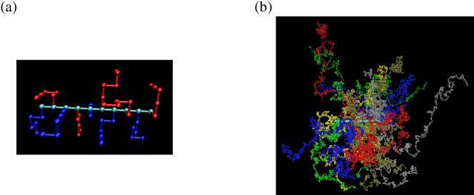
In the simple coarse-grained model, the backbone is fixed on the simple cubic lattice in the direction along the -axis. monomers of the backbone are located on the lattice sites as shown in Fig. 1. side chains consisting of monomers each are grafted to the backbone monomers with equal distance between two successive grafting sites on the backbone, where is the grafting density defined by . Since mainly we want to check the scaling laws for very long side chains, the periodic boundary condition is introduced in the direction along the backbone to avoid the end-effects associated with a finite backbone length. Differently from the conventional MC method where an initial configuration is set up as a starter for the simulation, the conformation of a bottle-brush polymer is built by growing all side chains simultaneously with PERM. The partition sum of bottle-brush polymers of side chains of length each,
| (1) |
is therefore the total number of all possible configurations of interactive self-avoiding random walks of steps . Only the excluded volume effect is considered here.
It is straight forward to apply the similar method for growing a star polymer Hsu2004 to the simulations for growing a bottle-brush polymer Hsu2007 . Only in the latter case, side chains can either be attached to the same site or the different sites on the backbone depending on the grafting densities. In the process of growing a bottle-brush polymer, one has to be aware that both the interactions between monomers in the same side chain, and the interactions between monomers on different side chains have to be taken into account. If one side chain is grown entirely before the next side chain is started, it will lead to a completely “wrong” direction of generating the configurations of a bottle-brush. Therefore, one has to use the strategy that all side chains are grown simultaneously. Namely, a monomer is added to each side chain step by step until all side chains having the same length, then that the next round of monomers is added. After we labelled all monomers by numbers, it goes back to the problem of growing a linear chains from the first monomer to the th monomer g97 . Using PERM, the configurations of bottle-brush polymers are built by adding one monomer at each step, and each configuration carries its own weight. A wide range of probability distributions can be used for selecting one of the nearest neighbor free sites of each side chain end at the next step, but the efficiency of the algorithm depends on the choice of the distribution. For the current problem, the bias of growing side chains is used by giving higher probabilities in the direction where there are more free next neighbor sites and in the outward directions perpendicular to the backbone, where the second part of bias decreases with the length of side chains and increases with the grafting density. The total weight for a bottle-brush polymer of all side chains having the length with an unbiased sampling is determined recursively by . As the weight is gained at the -step with a probability , one has to use instead of . By taking the average of all possible configurations, the partition sum
| (2) |
can be estimated directly, where is the total number of configurations . This is the main advantage of using PERM. For any observable , the mean value is therefore,
| (3) |
.

In order to suppress the huge fluctuation of the probability distribution and enrich those configurations with high weight the population control is made in the way of pruning low weight configurations and cloning those configurations with high weight. Two thresholds and are introduced,
| (4) |
where is the current estimate of the partition sum {Eq. (2)}, and and are constants of order unity. The optimal ratio between and is found to be in general. For our simulations, we use and for the first configuration hitting all side chains of length . For the following configurations, we use and , here , and is the total number of configurations of all side chains having length . If the current weight for the configuration , one produces two identical copies of this configuration, replaces their weight by . If , one calls a random number where . If , the configuration is kept but the weight is replaced by , while the configuration is killed if . Otherwise, the configuration is kept with the weight .
A typical configuration of bottle-brush polymers under a good solvent condition generated by PERM is shown in Fig. 1(b). It consists of backbone monomers, side chain monomers in each side chain, and the grafting density is . The total number of monomers is . So far, it is the largest bottle-brush polymers in the equilibrium state, generated by MC simulations Hsu2007 .
II.2 Bond fluctuation model with LPB
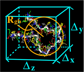
For studying bottle-brush polymers with a flexible backbone and flexible side chains, we generalize the bond fluctuation model for a linear polymer chain to that for a bottle-brush polymer. In the standard bond fluctuation model Carmesin1988 ; Deutsch1991 ; Paul1991 ; Binder1995 , a flexible polymer chain is described by a SAW on a simple cubic lattice with bond constraints. Each effective monomer blocks all 8 corners of an elementary cube of the lattice from further occupation. Two successive monomers along a chain are connected by a bond vector chosen from the set , , , , , , including also all permutations. The geometry of a bottle-brush polymer with backbone monomers, and with side chains of length is arranged in the way that side chains are added to the backbone chain at regular spacing , and two additional monomers are added to each chain end of the backbone. Thus, the total number of monomers is . For our simulations, one of the simplest ways to set up the initial configuration is to assume that the backbone and side chains all have rod-like structures. Placing the backbone along the -direction and fixing the bond length between two successive backbone monomers to be , and randomly choosing the bond vector of each side chain from one of the allowed bond vectors including all permutation in the xy-plane but keeping the bond vectors within each side chain fixed, the required condition of bond constraints is satisfied and no further check is needed. In our algorithm, instead of trying to move a chosen monomer to the nearest neighbor sites named by the local 6 (“L6”) moves for the standard bond fluctuation model, we use the local 26 (“L26”) moves Wittmer where it is tried to move to the neighbor sites as shown in Fig. 2(a). The local move is only accepted if the selected site is empty and the bond length constraints are satisfied. In addition, two types of pivot moves are attempted. One is that a monomer is chosen randomly on the backbone and the short part of the bottle-brush polymer is transformed by randomly applying one of the 48 symmetry operations (no change; rotations by and ; reflections and inversions). The other is that a monomer is chosen randomly from all side chain monomers, and the part of side chain from the selected monomer to the free end of the side chain is transformed by one of the 48 symmetry operations.
We first make some test runs for a small bottle-brush polymers with , , , , and , and in order to compare the efficiency between the “L26” moves and the “L26” moves + pivot moves. For any observable , the performance of the algorithm is determined by the autocorrelation function ,
| (5) |
Results of for the mean square gyration radius of the backbone, , and of the side chains, (taking the average of all side chains at the same MC step ) plotted against the number of MC steps show that the “L26” + pivot algorithm is two orders of magnitude faster than the “L26” algorithm for fixed side chain length (figures are not shown here). In the “L26” algorithm, one MC step consists of “L26” moves, i.e., each monomer is selected once for the local move. In the “L26” + pivot algorithm, one MC step consists of “L26” moves, times pivot moves of the backbone and times pivot moves of side chains. is chosen such that the acceptance ratio is about 40% or even larger, while is .
(a)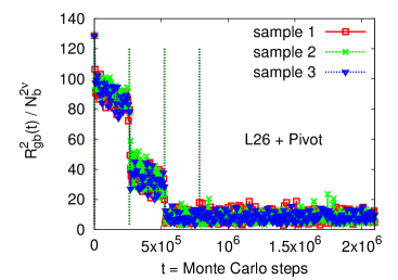 (b)
(b)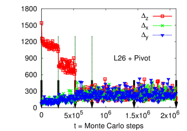
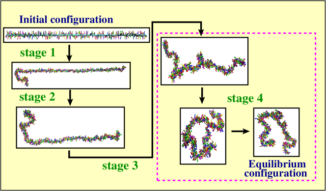
Two observables chosen for monitoring the equilibrating process as shown in Fig. 3 are the radius of gyration of the backbone monomers, , and the space occupation of the bottle-brush polymer in the Cartesian coordinates, , since the average conformations of bottle-brush polymers in equilibrium must be isotropic. For simulating small bottle-brush polymers, we can simply set the three orthogonal length scales in the Cartesian coordinates having equal length, e.g. in the equilibrating process. As the size of bottle-brush polymer increases, we will meet the problem of setting the simulation lattice box in our simulations due to the limitation of the computer memory. The maximum volume of the box is for those computers we can access. The solution for it is to adjust the simulation lattice box during the equilibrating process and separate the process into several stages. Let’s take a bottle-brush polymer with , , and as an example. The equilibrating process is separated into four stages as follows,
- stage 1:
-
, , , MC steps
- stage 2:
-
, , , MC steps
- stage 3:
-
, , , MC steps
- stage 4:
-
, , MC steps
Here is the pivot point selected from the backbone monomers. One has to be aware that the pivot points which can be selected for applying the pivot moves are also limited due to the current set up of the simulation lattice box. However, once the system is in equilibrium one has to allow all possible moves, i.e. . At every new stage , the initial configuration is taken from the last stage, and the size of the simulation lattice box is decided by the final space occupation of the bottle-brush polymers at the last stage, i.e. , , with , and . Time series of and are shown in Fig. 4. The four stages are separated by the vertical green curves. Taking some snapshots of the conformations of the bottle-brush polymers at the Monte Carlo steps indicated by the arrows in Fig. 4(b) one can see how the conformations of bottle-brush polymers change during the equilibrating process as shown in Fig. 5. At the beginning, backbone and side chains are in rod-like structures. At the end of the first stage, only a small part of the backbone is flexible. As more backbone monomers are relaxed, we see that the backbone and the side chains become more and more flexible step by step. Finally an equilibrium state is reached. It takes about hours CPU time on an Intel 2.8 GHZ PC for such a bottle-brush polymer to reach the equilibrium state by choosing and .
(a)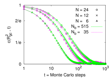 (b)
(b)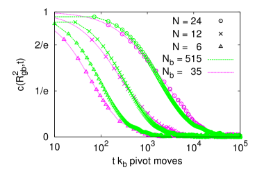
It is more time consuming when pivot moves are applied to the simulations for larger bottle-brush polymers. In order to know how much the efficiency is slowing down as the backbone length increases, we compare the autocorrelation functions and for bottle-brush polymers with and for three different side chain lengths , , and . For both cases in Fig. 6(a), we see that the decay of the autocorrelation function for the side chain structure occurs on the same time scale. It is also true for the backbone as shown in Fig. 6(b) that the autocorrelation functions are plotted against the number of pivot moves . Clearly, the structural relaxation time is longer as the side chain length increases Hsu2011 .
III Results
According to the cylindrical geometry of bottle-brush polymers with a rigid backbone, we extend the Daoud-Cotton blob picture for a star polymer to that for a bottle-brush polymer. The space is partitioned into blobs of non-uniform size and shape. The blobs are not spheres but rather ellipsoids. Based on this theory, the scaling law for side chains in the radial direction (height of the bottle-brush) is given by,
| (6) |
where is the Flory exponent for 3D SAWs (). With the first part of simulations by using PERM, results of the mean square height of bottle-brush polymers for three choices of backbone length , , and , and several choices of the grafting density from to are shown in Fig. 7(a). We see that those curves of the same grafting density coincide with each other. Increasing the grafting density enhances the stretching of side chains. Considering that in the mushroom regime , the height of bottle-brush polymers should behavior as 3D SAWs, i.e. , one can write down the scaling ansatz in the thermodynamic limit as Hsu2007 ,
| (7) |
with
| (8) |
For checking this cross-over scaling ansatz, we plot the same data as shown in Fig. 7(a), but rescale the x-axis from to . We see the nice data collapse. As increases, a cross-over from a 3D SAWs to a stretched side chain regime is indeed seen, but only rather weak stretching of side chains is realized, which is different from the scaling prediction {Eq. (6)}. In this log-log plot, the straight line gives the asymptotic behavior of the scaling prediction for very large . However, this is the first time we can see the cross-over behavior by computer simulations. This cross-over regime is far from reachable by experiments. On the other hand, it requires a lot of effort to reach the regime where the theoretical prediction would apply, either the grafting density has to be much higher or the side chain length has to be much longer.
(a)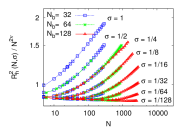 (b)
(b)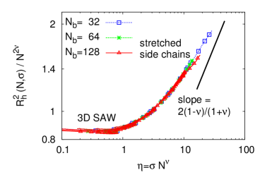
(a)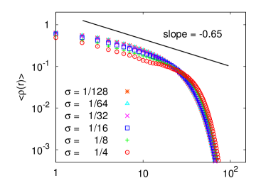 (b)
(b)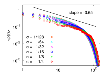

The same situation is also observed as we check the scaling prediction for the radial distribution function Hsu2007
| (9) |
Results are shown in Fig. 8 for bottle-brush polymers with side chain length and . As we keep all the grafting densities fixed but increase the side chain length , one can see only in a rather tiny regime, the data seem to follow the same slope as predicted by the theory. Therefore, one might expect that finally the radial distribution function would follow the predicted scaling law as both and are very large.
For the second part of the simulations, let’s first look at the snapshots of bottle-brush polymers under a good solvent condition, which contain backbone monomers, (linear polymer), , , and monomers on each side chain, and the grafting density . As increases, one sees that the corresponding conformations of bottle-brush polymers are rather different. The backbone becomes stiffer as the side chain length increases. This local intrinsic stiffness of the backbone is quantitatively described by the persistence length . According to the scaling law of the mean square end-to-end distance of the backbone Hsu2010a ; Hsu2010b ,
| (10) |
where is the average bond lengths for the bond fluctuation model. Results of the rescaled mean square end-to-end distance of the backbone for , , , , and and for various numbers of backbone monomers are shown in Fig. 10(a). The persistence length for fixed side chain length is determined by the plateau for large since finally those curves of all show a smooth cross-over from a rod-like chain to a 3D SAW. increases as increases.
The most common quantity to describe the structure of macromolecules is the structure factor for the whole bottle-brush polymer, which is estimated by taking the average of all independent configurations obtained from MC simulations, i.e.
| (11) |
where if is occupied, otherwise . In experiments, can be measured by using static light scattering, small angle neutron scattering, and x-ray scattering, e.g. Ref. Rath . By choosing the accessible size of bottle-brush polymers for experiments, we have found the connections between our MC simulation results and the experimental data Hsu2010a . One example is shown in Fig. 10(b). As we normalize the structure factor as , and rescale the wave factor to where is the radius of gyration of the whole bottle-brush polymer, we see that the backbone length in the experiment corresponds to the backbone length in the simulation, and side chain length in the experiment corresponds to the side chain length in the simulation. The grafting density for both cases. Immediately, we can translate that nm lattice spacings.
(a)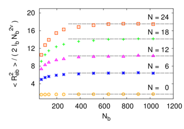 (b)
(b)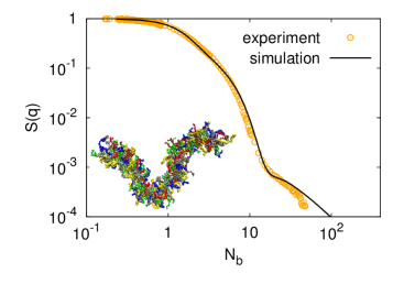
IV Conclusions
In this paper, we study the bottle-brush polymers under good solvent conditions by using two kinds of lattice models, a simple coarse-grained model on the simple cubic lattice and the bond fluctuation model. Due to the complex characteristics of bottle-brush polymers, we have proposed two algorithms, a variant of PERM and LPB depending on the interesting regime of length scales. With our extensive MC simulations, we show that the stretching of side chains in the interior of the bottle-brush polymer is weaker than the theoretical prediction. A convincing estimate of the persistence length which describes the intrinsic stiffness of bottle-brush polymers depending on the side chain length is given. We also give a direct comparison of the structure factors between our simulation results and the experimental data. The newly developed algorithm LPB has also been employed successfully to study the conformational change of bottle-brush polymers as they are adsorbed on a flat solid surface by varying the attractive interaction between the monomers and the surface Hsu2010c .
Acknowledgement
H.-P. H. received funding from the
Deutsche Forschungsgemeinschaft (DFG), grant No SFB 625/A3.
We are grateful for extensive grants of computer time at the JUROPA
under the project No HMZ03 and
SOFTCOMP computers at the Jülich Supercomputing Centre (JSC),
and PC clusters at ZDV, university of Mainz.
H.-P. H. thanks K. Binder and W. Paul for their kind support and
collaboration.
References
References
- (1) Y. Rouault, O. V. Borisov: Macromolecules 29, 2605 (1996).
- (2) Y. Rouault: Macromol. Theory Simul. 7, 35 (1998).
- (3) K. Shiokawa, K. Itoh, N. Nemoto: J. Chem. Phys. 111, 8165 (1999).
- (4) M. Saariaho, O. Ikkala, I. Szleifer, I. Erukhimovich, G. ten Brinke: J. Chem. Phys. 107, 3267 (1997).
- (5) S. Elli, F. Ganazzoli, E. G. Timoshenko, Y. A. Kuznetsov, R. Connolly: J. Chem. Phys. 120, 6257 (2004).
- (6) A. Yethiraj: J. Chem. Phys. 125, 204901 (2006).
- (7) H.-P. Hsu, W. Paul, S. Rathgeber, K. Binder: Macromolecules 43, 1592 (2010).
- (8) H.-P. Hsu, W. Paul, K. Binder: Macromolecules 43, 3094 (2010).
- (9) P. Grassberger: Phys. Rev. E 56, 3682 (1997).
- (10) H.-P. Hsu, W. Nadler, P. Grassberger: Macromolecules 37, 4658 (2004).
- (11) H.-P. Hsu, W. Paul, K. Binder: Macromol. Theotry & Simul. 16, 660 (2007).
- (12) I. Carmesin, K. Kremer: Macromolecules 21, 2819 (1988).
- (13) H. P. Deutsch, K. Binder: J. Chem. Phys. 94, 2294 (1991).
- (14) W. Paul, K. Binder, D. W. Heermann, K. Kremer: J. Phys. II 1, 37 (1991).
- (15) K. Binder (editor): Monte Carlo and Molecular Dynamics Simulations in Polymer Science”, p1 (Oxford Univ. Press, New York, 1995).
- (16) H.-P. Hsu, K. Binder, W. Paul: Phys. Rev. Lett. 103, 198301 (2009).
- (17) J. P. Wittmer, P. Beckrich, H. Meyer, A. Cavallo, A. Johner, J. Baschnagel: Phys. Rev. E 76, 011803 (2007).
- (18) H.-P. Hsu, W. Paul: preprint (2011).
- (19) S. Rathgeber, T. Pakula, K. Matyjaszewski, K. L. Beers: J. Chem. Phys. 122, 124904 (2005).
- (20) H.-P. Hsu, W. Paul, K. Binder: J. Chem. Phys. 133, 134902 (2010).