A review of Monte Carlo simulations of polymers with PERM

Abstract

In this review, we describe applications of the pruned-enriched Rosenbluth method (PERM), a sequential Monte Carlo algorithm with resampling, to various problems in polymer physics. PERM produces samples according to any given prescribed weight distribution, by growing configurations step by step with controlled bias, and correcting “bad” configurations by “population control”. The latter is implemented, in contrast to other population based algorithms like e.g. genetic algorithms, by depth-first recursion which avoids storing all members of the population at the same time in computer memory. The problems we discuss all concern single polymers (with one exception), but under various conditions: Homopolymers in good solvents and at the $\Theta$ point, semi-stiff polymers, polymers in confining geometries, stretched polymers undergoing a forced globule-linear transition, star polymers, bottle brushes, lattice animals as a model for randomly branched polymers, DNA melting, and finally – as the only system at low temperatures, lattice heteropolymers as simple models for protein folding. PERM is for some of these problems the method of choice, but it can also fail. We discuss how to recognize when a result is reliable, and we discuss also some types of bias that can be crucial in guiding the growth into the right directions.

I Introduction

Research in the field of polymer physics has grown vigorously since the 1950s Flory ; Lifshitz ; deGennes ; Grosberg . Recent developments in the techniques for the tools of atomic force microscopy (AFM) Roiter , in fabrication of nanoscale devices and in single-chain manipulation techniques Salman ; Meller ; Kasianowicz open possibilities for a broad range of applications in physical chemistry, biotechnology and material science. During this time, much effort has also been put into studying the statistical properties of polymers by computer simulations Binder ; Binder08 . Indeed, due to the richness of the observed phenomena and the non-triviality of the problems involved, polymer physics has from the very beginning served as a playground for developing novel Monte Carlo strategies RR ; Wall-Erpenbeck ; Madras-Sokal . These strategies depend strongly on the problems one is interested in: Linear versus branched polymers, dilute versus dense systems, scaling laws versus detailed material properties, classical versus quantum mechanical problems, implicit versus explicit treatment of solvent, etc.

In this review we shall only deal with one class of algorithms, the pruned-enriched Rosenbluth method (PERM) Grassberger97 . So far it has been used for classical physics only, although closely related methods have also been used since long ago for quantum mechanical simulations Anderson . Although it is not a panacea and fails miserably in many problems, it still found applications to several of the above dichotoma, and in some cases it beats the (presently known) competitors by huge margins.

In the following we shall mostly be concerned with single unbranched molecules moving freely in a dilute solvent. Later we will also consider branched polymers and polymers attached to surfaces. The basic characteristics of linear polymer chains depend on the solvent conditions. At high temperatures or in good solvents repulsive interactions (the excluded volume effect) and entropic effects dominate the conformation, and the polymer chain tends to swell to a random coil. At low temperatures or in poor solvents, however, attractive interactions between monomers dominate the conformation and the polymer chain tends to collapse and form a compact dense globule. The coil-globule transition point is called the $\Theta$-point. Based on field theory deGennes , the behavior of polymer chains in good solvents is well understood. In the thermodynamic limit (as the chain length $N\rightarrow\infty$), the partition function scales as

$$Z\sim\mu_{\infty}^{-N}N^{\gamma-1}\enspace{\rm at}\enspace T>T_{\Theta}$$ (1)

where $\mu_{\infty}$ is the critical fugacity and $\gamma$ is the entropic exponent related to the topology. Below the $\Theta$-point, a collapsed polymer can essentially be viewed as a liquid droplet. According to the Lifshitz mean field theory Lifshitz ; Grosberg , a surface term should be included in the partition sum as

$$Z\sim a^{N}b^{N^{s}}N^{\gamma-1}\enspace{\rm at}\enspace T<T_{\Theta}$$ (2)

with $s=(d-1)/d$ and $b>1$.

Generally speaking, the thermodynamic limit of a polymer system coincides with the limit when the chain length $N$ tends to infinity. For conventional Monte Carlo (MC) methods such as the Metropolis algorithm, one can only simulate moderately large systems, the maximal feasible values of $N$ depending on the temperature and on the degree of reality of the model. Going from simple lattice-based models at high temperatures to models with realistic interactions and further to folded proteins with explicitly included solvent, $N_{\rm max}$ might decrease from $10^{4}$ to $\ll 100$. If one is interested mostly in scaling laws (as we shall be), one simulates at several values of $N$ and uses finite-size scaling (FSS) to extrapolate the behavior of the considered thermodynamic quantities to $N\rightarrow\infty$. Rather often, either very large finite-size effects have to be considered or it is too difficult to reach equilibrium states or to produce sufficiently many independent configurations. For some problems (not for all!), it was a big breakthrough when (PERM) Grassberger97 ; Grassberger98 ; GN00 ; Grassberger02 was proposed in 1997. It is particularly efficient for temperatures near the $\Theta$ collapse, where chains of length up to $N=1,000,000$ could be sampled with high statistics, and it was confirmed unambiguously that the $\Theta$ collapse is a tricritical phenomenon with upper critical dimension $d_{c}=3$ deGennes . Since then, many other applications have also been made. Many other applications have also been made successfully by PERM Grassberger02 , which provide in some cases a deep understanding on the scaling behavior of polymer chains under different solvent conditions, geometrical confinements, on the phase transition behavior of polymer chains adsorbed onto a wall, on polymers stretched by a force, etc.

In the next section we give a detailed description of the basic algorithm. This algorithm can be made substantially more efficient by a suitable bias in the growth direction, and two biases (including ‘Markovian anticipation’) are discussed in Sect. 3. Applications are treated in Sects. 4 ($\Theta$-polymers), 5 (stretched polymers in poor solvents), 6 (semiflexible polymers), 7 (polymers in confining geometries), 8 (branched polymers with fixed tree topologies), 9 (lattice animals), 10 (protein folding), and 11 (DNA melting). Finally the paper concludes with a summary in Sect. 12.

Figure 1: Schematic drawings of building a SAW from the $0^{\rm th}$ step to the $4^{\rm th}$ step and the associated weight at each step. At the $0^{\rm th}$ step, we set the weight $W_{0}=w_{0}=1$, and the probability $p_{0}=1$. The Rosenbluth bias is used here such that $p_{n}=1/n_{\rm free}$ at each step, so the total weight $W_{n}=\Pi_{n=0}^{n=4}n_{\rm free}$.

II Algorithm: Pruned-enriched Rosenbluth Method (PERM)

In statistical thermodynamics, the partition function for a canonical ensemble in thermal equilibrium is defined by

$$Z(\beta)=\sum_{\alpha}Q(\alpha)=\sum_{\alpha}\exp(-\beta E(\alpha))$$ (3)

here $\beta=1/k_{B}T$, $E(\alpha)$ is the corresponding energy for the $\alpha^{\bf th}$ configuration, $Q(\alpha)/Z$ is the Gibbs-Boltzmann distribution, and $Q(\alpha)=\exp(-\beta E(\alpha))$ is normally called the Boltzmann weight. If each configuration is repeatedly and independently chosen according to a randomly chosen probability $p(\alpha)$ (a bias), the partition sum is rewritten as

$$Z=\lim_{M\to\infty}\hat{Z}$$ (4)

where $M$ is the number of trials and

$$\hat{Z}=\frac{1}{M}\sum_{\alpha=1}^{M}Q(\alpha)/p(\alpha)=\frac{1}{M}\sum_{\alpha=1}^{M}W(\alpha)\;,$$ (5)

with modified weights

$$W(\alpha)=Q(\alpha)/p(\alpha).$$ (6)

If we use $p(\alpha)\propto\exp(-\beta E(\alpha))$ {Gibbs sampling}, each contribution to $\hat{Z}_{M}$ has the same weight, which is an example of the so called ‘importance sampling’. The estimate for any observable $A$ is given by

$$\langle A\rangle=\lim_{M\to\infty}\langle A\rangle_{M}=\lim_{M\to\infty}\frac{\sum_{\alpha=1}^{M}A(\alpha)W(\alpha)}{\sum_{\alpha=1}^{M}W(\alpha)}\;.$$ (7)

In general, we expect that statistical fluctuations of $\langle A\rangle_{M}$ are minimal, at given $M$, if we use importance sampling and if all trials are independent. In general this is infeasible. The Metropolis method achieves perfect importance sampling at the cost of highly correlated trials. PERM tries, with a completely different strategy, at a compromise between importance sampling and independence.

Things are best illustrated by a linear chain of $N+1$ monomers in an implicit solvent, modeled by an interacting self-avoiding walk (ISAW) of $N$ steps on a simple (hyper-)cubic lattice of dimension $d$. The interactions in this model are (i) the chain connectivity which enforces that adjacent monomers sit on adjacent lattice sites; (ii) self-avoidance that excludes configurations in which the same lattice site is occupied by two or more monomers; and attractive interactions (energies $\epsilon<0$) between non-bonded monomers occupying neighboring lattice sites. Writing $q=\exp(-\beta\epsilon)$ for the Boltzmann factor, the partition sum is

$$Z_{N}(q)=\sum_{\rm walks}q^{m}$$ (8)

where $m$ denotes the total number of non-bonded nearest neighbor pairs. The solvent quality is varied by changing the temperature $T$.

In the original Rosenbluth-Rosenbluth (RR) method RR , polymer chains are built like random walks by adding one monomer at each step. At the $0^{\rm th}$ step, the first monomer is placed at an arbitrary lattice site. For this “chain” of length $N=0$, the weight is trivially $W_{0}=1$. For the first step one has $2d$ possibilities and no interactions yet, giving $W_{1}=2d$. For subsequent steps one has to take self-avoidance into account. When a monomer is added to a chain of length $N-1$, one scans the neighborhood of the chain end to identify the free sites on which a monomer could be added. If there are $n_{\rm free}\geq 1$ free neighbors, the next step is chosen uniformly among them, while the walk is killed if $n_{\rm free}=0$ (“attrition”). After this step the weight $W_{N}$ is updated by multiplying $W_{N-1}$ by

$$w_{n}=q^{m_{n}}/p_{n},$$ (9)

where $p_{n}=1/n_{\rm free}$ and $m_{n}$ is the number of neighbors of the new site already occupied by non-bonded monomers (notice that $m=\sum_{n=0}^{N}m_{n}$). Therefore, after $N$ steps the total weight is

$$W_{N}=w_{N}W_{N-1}=\ldots=w_{N}w_{N-1}\dots w_{0}=\prod_{n=0}^{N}w_{n}\;.$$ (10)

When the chain length $N$ becomes very large, the method fails for two reasons: First of all, attrition implies that only an exponentially small fraction of trials survive and give any contribution at all. Secondly, as the weight factors $w_{n}$ are weakly correlated random variables, the full weight $W_{N}$ will show huge fluctuations. Thus the surviving configurations will finally be dominated by a single configuration, demonstrating a dramatic lack of importance sampling.

PERM Grassberger97 was invented to overcome this shortcoming of the RR method. The main spirit of PERM is as follows,

• Polymer chains are built like random walks by adding one monomer at each step.

• A Rosenbluth-like bias is used for choosing one of the nearest neighbor free sites for the next step of the walk, but a wide range of probability distributions can be used depending on the specific problem at hand, which will be discussed in detail in the following sections.

• In order to overcome attrition and to reduce the fluctuations of $W_{n}$, one uses “population control”. This is achieved by pruning some low-weight configurations and cloning (“enriching” Wall-Erpenbeck ) all those with high weight, as the chain grows. To define ‘low’ and ‘high’ weights, one uses two thresholds $W_{n}^{+}$ and $W_{n}^{-}$. If at any step $n$ the current weight $W_{n}$ according to (10) would be $>W_{n}^{+}$, we make $k$ additional copies (typically $k=1$) of the current configuration and give each copy a weight $W_{n}=w_{n}W_{n-1}/(k+1)$. On the other hand, if (10) would give $W_{n}<W_{n}^{-}$, we call a random number $r\in\left[0,1\right]$. If $r<1/2$ we kill the configuration. Otherwise, we keep it and double its weight, $W_{n}=2w_{n}W_{n-1}$. It is easy to see that pruning and cloning leave all averages unchanged. It improves importance sampling enormously, but it also leads to correlated trials.

  For most problems the choice of the thresholds $W_{n}^{+}$ and $W_{n}^{-}$ is unproblematic, and they can be chosen simply as constant multiples of the the current estimate of the partition sum given by (5),

  $$W_{n}^{+}=C_{+}\hat{Z}_{n}\qquad{\rm and}\qquad W_{n}^{-}=C_{-}\hat{Z_{n}}\;,$$ (11)

  were $C_{+}$ and $C_{-}$ are constants of order unity. A good choice for the ratio between $C_{+}$ and $C_{-}$ is found to be $C_{+}/C_{-}\sim 10$ in most cases. If (11) does not lead to good results, chances are that the method would not work with any other choice either. If the method works well, (11) gives samples where the total number of length $n$ configurations is independent of $n$, i.e. attrition is completely eliminated and pruning & cloning compensate each other exactly (up to statistical fluctuations), for large $n$. For the first trials (when there is not yet any estimate $\hat{Z}_{n}$), we choose normally $W_{n}^{-}=0$ and $W_{n}^{+}=\infty$ (a very large number like $10^{100}$), which gives the original RR method.

• The copies made in the enrichments are placed on a stack, and a depth-first implementation is used for the chain growth: At each time one deals with only a single configuration until a chain has either grown to the maximum length $N$ or has been killed due to attrition. If the first happens or if the stack is empty, a new trial is started. Otherwise, the configuration on top of the stack is popped and the simulation continues. This is most easily implemented by recursive function calls. Since only a single configuration has to be remembered during the run, this requires much less memory than a breadth-first implementation that uses an explicit “population” of many configurations, as it is traditionally used e.g. in genetic algorithms.

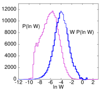
  (a)               (b)

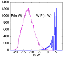
  Figure 2: Histograms of logarithms of tour weights $P(\ln W)$ normalized as tours per bin, and weighted histograms $WP(\ln W)$ are shown as indicated. Weights $W$ are only fixed up to a $\beta$-dependent multiplicative constant. The simulation shown in panel (a) is reliable, while that in panel (b) is not. Adapted from Ref. PW-G99 .

• As we said, configurations obtained from different clones of the same ancestor will not be uncorrelated. The set of all such configurations is called a “tour”. Different tours are uncorrelated. Depending on the amount of cloning/pruning, however, the correlations within a tour could be so strong as to render the method obsolete. In that case the distributions $P(\ln({\cal W}))$ of logarithms of tour weights ${\cal W}$ is very broad, so that we are basically back to the problem of the RR method (with single trials replaced by tours): Averages might be dominated, in extreme cases, by a single tour. For checking against this, we simply look at $P(\ln({\cal W}))$ (see Fig. 2), and compare it with the weighted distribution ${\cal W}P(\ln{\cal W})$. If ${\cal W}P(\ln{\cal W})$ has its maximum at a value of $\ln{\cal W}$ where the distribution $P(\ln{\cal W})$ is well sampled, we are on the safe side. If not, then the results can still be correct, but we have no guarantee for it. An illustration of these two cases is shown in Fig. 2 PW-G99 . Fig 2(a) shows that the sampling is sufficient and the statistical weight distribution is reliable, but Fig. 2(b) shows the opposite situation where the result might be completely wrong.

III Biased Growth

An important aspect of the method is that in general, for high efficiency, one should choose judiciously a bias in the growth, in order to reduce as much as possible the fluctuations of the weight factors $w_{n}$. The optimal choice of bias is often a result of trial and error, as there exists no general theory for it. The two choices discussed in the following subsections are often useful, but by no means in all cases – and other choices may be useful in other applications.

One aspect of PERM that often decides the success or failure is that any bias that improves the growth at an intermediate stage should also be helpful later, i.e. it should not lead the growth into a dead end. One application where this is violated dramatically is e.g. the problem of random walkers in a medium with randomly placed traps (the “Wiener sausage” problem, leading to the famous Donsker-Varadhan stretched exponential survival probability Donsker ). In this problem walkers should, to maximize their survival chance at very long times, stay very close to their starting point. On the other hand, for short times the path integral (partition sum) is dominated by walkers who venture out to explore a larger area, even if that might mean they get killed by a trap. Since this system can be mapped onto a polymer problem, one can apply PERM to it Mehra . These PERM simulations gave indeed the first unambiguous numerical verification of the Donsker-Varadhan law, nevertheless they completely failed for very long times, because both bias and population control conspired to “mislead” the walkers Mehra to venture too far out.

III.1 Global Directional Bias

Assume you want to simulate a polymer whose one end is held fixed at ${\bf x}=0$, and the other end is pulled away by a constant force ${\bf F}$. In Sect. V we shall discuss in detail the case of a poor solvent where the stretching might unfold the dense globule into which the unstretched polymer would collapse. Here we just discuss qualitatively a polymer in a good solvent, i.e. a stretched SAW.

This system could of course be simulated by an unbiased SAW, and the stretching could be taken into account by reweighing each obtained configurations with a Boltzmann weight $\propto\exp(-\beta{\bf x\cdot F})$. But this would be extremely inefficient for large $F$, since weights would be very uneven, and “correct” configurations would be very rare and would have very high weight.

A much better strategy is to use a bias in the direction of the next step of the walk in the direction of ${\bf F}$. The amount of the optimal bias cannot be determined a priori, but depends also on the excluded volume effect which helps to push the end further away in the direction of the bias. We do not show any data here, but we just mention that the simulations get easier with increasing $F$, since the walk resembles more and more an ordinary biased walk in this limit, and pruning/cloning events get more and more rare.

III.2 PERM with $k$-step Markovian anticipation

A less trivial bias is suggested by the fact that a growing polymer will predominantly grow away from the already existing part of the chain. This could be modeled crudely by determining the center of mass of that part, and biasing the growth away from it. A better strategy is to learn on the fly how a typical short existing chain (of $k$ monomers, say) would bias the further growth in detail, and to remember at any time the previous $k$ steps. This is called Markovian anticipation Grassberger98 ; Frauenkron99 ; Strip ; Slab .

The crucial point of the $k$-step Markovian anticipation is that the $(k+1)^{\rm th}$ step of walk is biased by the history of the previous $k$ steps, i.e., the bias depends on the last $k$ steps. Let’s consider the general case of a walk on a $d$-dimensional hypercubic lattice. At each step $i$, a walk can move towards to one of the $2d$ directions denoted by $s_{i}=0$, $\ldots$, $2d-1$. All possible configurations of $(k+1)$ steps ($i=-k$, $-k+1$, $\ldots$, $-1$, and $0$), which are in total $(2d)^{k+1}$ configurations, are labelled by

$$\bf S=(s_{-k},\;\ldots,\;s_{-1},\;s_{0})=({\bf s},\;s_{0})$$ (12)

here ${\bf s}$ and $s_{0}$ denote the configurations of the previous $k$ steps and the $(k+1)^{\rm th}$ step, Either during a separate auxiliary run or during the first part of a long run we build a histogram $H_{m}({\bf S})$ with $(2d)^{k+1}$ entries. For any ${\bf S}$, the value of $H_{m}({\bf S})$ is the sum of all contributions to ${\hat{Z}}_{n+m}$ of configurations that had coincided with ${\bf S}$ during the steps $n-k$, $n-k+1$, $\ldots$, and $n$, summed over all $n$ in some suitable range excluding transients. Typical values for 3-d SAWs might be $k=10,m=100,n>300$. Then $H_{m}({\bf S})/H_{0}({\bf S})$ measures how successful configurations ending with ${\bf S}$ were in contributing to the partition sum $m$ steps later. The bias in $k$-step Markovian anticipation for the next step is thus defined by

$$P(s_{0}|{\bf s})=\frac{H_{m}({\bf s},s_{0})/H_{0}({\bf s},s_{0})}{\sum_{s_{0}^{\prime}=0}^{2d-1}H_{m}({\bf s},s_{0}^{\prime})/H_{0}({\bf s},s_{0}^{\prime})}\;.$$ (13)

IV $\Theta$-Polymers

The first application of PERM was to $\Theta$-polymers in three dimensions Grassberger97 . As we said, the upper critical dimension for the $\Theta$ collapse is $d=3$, whence we expect ordinary random walk behavior with logarithmic corrections. These corrections have been calculated to leading Duplantier-Theta and next-to-leading Hager orders. The experimental verification of these corrections is highly non-trivial, because one has to use extremely diluted solutions in order to avoid coagulation of different chains, and thus the signals are very weak. Nevertheless, they have been observed in small-angle neutron scattering Boothroyd .

IV.1 A Single $\Theta$-Polymer

It is for this problem that PERM shows the biggest improvement over all other Monte Carlo methods. The reason is that at the $\Theta$ point entropic and energetic (Boltzmann-) effects cancel exactly in the limit $N\to\infty$. For finite $N$ they do not cancel exactly (this gives rise to the logarithmic corrections), but it is still true that the weight factors $w_{n}$ are very close to 1. Thus hardly any pruning/cloning is needed, and to a first approximation the simulation reduces simply to a straightforward simulation of random walks with small weight corrections. Full PERM simulations for very long chains (the longest chains in Grassberger97 had $N=10^{6}$) do require in average one pruning/cloning step for every 2000 ordinary random walk steps. Therefore, in chain length $n$ the algorithm effectively performs a random walk with diffusion coefficient $D\approx 2000$. Asymptotically for $N\to\infty$ the algorithm still needs ${\cal O}(N^{2})$ steps to create one independent configuration of full length, but the coefficient is tiny.

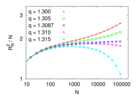
(a)     (b)

Figure 3: The mean square end-to-end distance $R_{N}^{2}$ plotted against $N$ in a log-log scale (a) and against $1/\ln N$ in the normal scale (b) Grassberger97 . $R^{2}/N\propto 1-37/(363\ln N)$ is indicated by the straight line. Adapted from Ref. Grassberger97 .

Indeed, since a growing polymer with endpoint in a locally denser region might feel an elevated Boltzmann factor at step $n$, but feels the compensating entropic disadvantage only one step later, the optimal algorithm that produced these results was a slight modification of the algorithm described in the previous section, where the population control was based on a modified weight with incremental weight factors

$$w^{\prime}_{n}=q^{m_{n}}/p_{n+1}.$$ (14)

instead of (9). Results are shown in Fig. 3. Theory Duplantier-Theta predicts leading logarithmic corrections to be $R_{N}^{2}/N\propto 1-37/(363\ln N)$, which would be a straight line in Fig. 3(b) with very small negative slope. Compared to that, the corrections to random walk behavior seen in Fig. 3(b) are much larger, although they are clearly smaller than one would expect for, say, a power law correction. It was indeed shown in Hager that the next-to-leading term increases the deviation from mean field behavior and improves thus the agreement between theory and simulation, but a fully quantitative verification remains elusive.

Far below the $T_{\Theta}$, PERM becomes inefficient, and it is instructive to see why: In strongly collapsed globules, polymer configurations are locally similar to those in a dense melt, and are well approximated by simple random walks without any correlations deGennes . But this implies that a collapsed chain with $N=1000$ has a configuration that is completely different from the first $1000$ monomers of, say, a collapsed chain of 8000 monomers. The former would form a compact globule, while the latter would form a rather dilute structure. Thus, similar to the problem discussed at the end of the last section, bias and population control during the early stages of growth would be completely misleading as far as late stages of growth are concerned. Otherwise said, by effectively disallowing configurations that are initially dilute and fill the interior only during the later growth, the entropy is severely underestimated.

IV.2 Unmixing Transition of Semidilute Solutions of very long Polymers

Let us now consider a semidilute solution of polymers of common length $N$ slightly below the $T_{\Theta}$ temperature. The “unmixing” transition at which these polymers coagulate and phase separate from the solute is, for any finite chain length $N$, in the Ising universality class Widom . As $N\to\infty$, the transition temperature $T_{c}$ should approach $T_{\Theta}$ from below. Since the Ising model has upper critical dimension $d_{c}=4$, but the $\Theta$-point has upper critical $d_{c}=3$, all critical exponents referring to collective properties (correlation length, specific heat) should be that of the Ising model, while properties characterizing the $N$-dependence (e.g. radii of gyration, critical concentration, $T_{\Theta}-T_{c}$) should be mean field like with logarithmic corrections. In particular, the monomer density at the critical point should scale as

$$\Phi_{c}\sim N^{-1/2},$$ (15)

up to logarithms of $N$.

A long standing problem in the 1990’s was that all experiments showed $\Phi_{c}\sim N^{-x_{c}}$ with $x_{c}=0.38\pm 0.01$ Widom , which was considered as incompatible with theory – in particular, since experimenters viewed any prediction of logarithmic corrections with great skepticism.

PERM can be easily modified for multi-chain systems, simply by placing the first monomer of a new chain not near the end of the last chain, and by applying the correct combinatorial factors that take into account the identities of different chains Frauenkron-unmix . Such simulations are very inefficient for short chains, since then $T_{c}\ll T_{\Theta}$, but they become more and more efficient as $N\to\infty$. They showed clearly that the deviations from (15) are not due to a different critical exponent, as was believed at this time, but due to logarithmic corrections Frauenkron-unmix . These are much larger than predicted by theory Duplantier92 , but this was to be expected in view of the results for single isolated chains.

V Stretching Collapsed Polymers in a Poor Solvent

As a collapsed polymer chain of chain length $N$ is stretched by an external force under poor solvent conditions, one observes from a collapsed globule phase to a stretched phase, as the stretching force is increased beyond a critical value Stretch . This phase transition is first order in $d=3$ dimensions, as is also suggested by the analogy of the Rayleigh instability of a falling stream of fluid, but it seems to be second order in $d=2$ Stretch . Here we shall only discuss the 3-d case.

This is modeled as a biased interacting self-avoiding random walk (BISAW) on a simple cubic lattice in three dimensions. Assuming that a chain is stretched in the x-direction by the stretching force ${\bf F}=F\hat{e}_{x}$ ($\hat{e}_{x}$ is the unit vector in the x-direction), an additional bias term $b^{x}$ is incorporated into the partition sum given by (8), where $b=\exp(\beta aF)$ is the stretching factor ($a$ is the lattice constant) and $x$ is the distance (in units of lattice constants) between the two end points of the chain in the direction of ${\bf F}$. The partition sum is therefore

$$Z_{N}(q,b)=\sum_{walks}q^{m}b^{x}\;.$$ (16)

The poor solvent condition is indicated by $q>q_{\Theta}$ where $q_{\Theta}=e^{-\epsilon/kT_{\Theta}}\approx 1.3087(3)$ Grassberger97 . According to the scaling law (2), in the thermodynamic limit $N\rightarrow\infty$, the partition sum for polymers in a poor solvent scales as

$$-\ln Z_{N}(q,b=1)\approx\mu_{\infty}(q)N+\tilde{\sigma}(q)N^{2/3}-(\gamma-1)\ln N$$ (17)

with $\mu_{\infty}$ being the chemical potential per monomer in an infinite chain, and $\tilde{\sigma}$ is related to the surface tension $\sigma$.

Choosing $q=1.5$ which is deep in the collapsed region, we performed simulations of BISAW with PERM. In order to improve the efficiency, each step of a walk is guided to the stretching direction with a higher probability. The $n^{th}$ step of walk (adding the $(n+1)^{\rm th}$ monomer) is toward one of the free nearest neighbor sites of the $n^{\rm th}$ monomer in the parallel, antiparallel, and transverse direction to ${\bf F}$ with probability: $p_{+}:p_{-}:p_{\perp}=\sqrt{b}:\sqrt{1/b}:1$. Thus we have

$$p_{i}=\left\{\begin{array}[]{ll}0&{\rm if\;the\;step\;of\;the\;walk\;toward\;to}\\ &{\rm the\;{\it i}-direction\;is\;forbidden}\\ \frac{p_{i}^{(0)}}{\sum_{{\rm allowed}\,j}p_{j}^{(0)}}&{\rm otherwise}\end{array}\right.$$ (18)

The corresponding weight factor at the $n^{th}$ step is then

$$w_{i_{n}}=\frac{q^{m_{n}}b^{\Delta x_{i}}}{p_{i}}\;,$$ (19)

where $m_{n}$ is the number of non-bonded nearest neighboring pairs of the $(n+1)^{\rm th}$ monomer. $\Delta x_{i}=0$, $1$ or $-1$ if the displacement $({\bf r}_{n+1}-{\bf r}_{n})$ between the $(n+1)^{\rm th}$ and $n^{\rm th}$ monomers is in the direction perpendicular, parallel, and antiparallel to ${\bf F}$, respectively. The total weight of a chain of length $n$ is then

$$W_{n}=\prod_{n^{\prime}=0}^{n}w_{i_{n^{\prime}}}\;.$$ (20)

Using (5) and (11), chains are cloned and pruned if their weight is above $3\hat{Z}_{n}$ and below $\hat{Z}_{n}/3$, respectively.

(a)     (b)

Figure 4: (a) $\ln Z_{N}(q,b)+\mu_{\infty}N$ for $d=3,q=1.5$, and for various values of $b$. The value $\mu_{\infty}=-1.7530\pm 0.0003$ used in this plot was obtained from dense limit simulations on finite lattices Stretch . (b) Histograms of the end point distance $P(x)$ versus $x/N$ for $q=1.5$. Biases were adjusted so that both peaks have equal height: $b=1.4040\;(N=500)$, $1.4925\;(N=1000)$, $1.5386\;(N=1500)$, $1.5658\;(N=2000)$, $1.5855\;(N=2500)$. Normalization is arbitrary. The peak at $x/N\approx 0$ corresponds to the collapsed phase, the other one to the stretched phase. Adapted from Ref. Stretch .

Results of $\ln Z_{N}(q,b)+\mu_{\infty}N$ plotted against $N$ are shown in Fig. 4(a) for various values of $b$. For small $b$ the curves are close to the curve for $b=1$. As $b$ increases, the initial (small-$N$) parts of these curves are straight lines with less and less negative slopes. In this regime the polymer is stretched. As long as these slopes are negative, the straight lines will intersect the curve for $b=1$ at some finite value of $N$, say $N_{c}(b)$, i.e. for the finite system of chain length $N_{c}(b)$ the corresponding effective transition point is $b$. For $N>N_{c}(b)$, the values of $\ln Z_{N}(q,b)+\mu_{\infty}N$ must deviate from the straight lines { see Refs. Mehra and Stretch } for the detailed explanations. Since the curve for $b=1$ becomes horizontal for $N\to\infty$, the true phase transition occurs at that value of $b$ for which the straight line in Fig. 4(a) is also horizontal. This can be estimated very easily and with high precision, giving for $q=1.5$ our final estimate $b_{c}\approx 1.856(1)$.

To clarify that the transition is indeed a first-order phase transition, one can study the histograms of $x$ and $m$ since PERM gives direct estimates of the partition sum and of the properly normalized histograms. The general formula of the histogram is

$$P_{q,b}(m,x)=\sum_{walks}q^{m^{\prime}}\,b^{x^{\prime}}\,\delta_{m,m^{\prime}}\delta_{x,x^{\prime}}\;.$$ (21)

Reweighting histograms obtained with runs performed nominally at $q^{\prime}$ and $b^{\prime}$ is trivially done by

$$P_{q,b}(m,x)=P_{q^{\prime},b^{\prime}}(m,x)(q/q^{\prime})^{m}(b/b^{\prime})^{x}\;.$$ (22)

Combining results from different runs can then be either done by selecting for each $(m,x)$ just the run which produced the least noisy data (which was done here in most cases), or by assuming that the statistical weights of different runs are proportional to the number of “tours” Grassberger97 which contributed to $P_{q,b}(m,x)$. Note that for conventional Metropolis-type Monte Carlo algorithms, it is not trivial to combine MC results from different temperatures since the absolute normalization is unknown ferrenberg .

An example of histograms $P(x)$ for fixed $q=1.5$ and $b$, plotted against $x/N$ are shown in Fig. 4(b) for $N=500$, $1000$, $1500$, $2000$, and $2500$. The value of $b$ is determined such that the two peaks have the same height for each $N$, i.e., $b_{c}(N)=b$ is the effective transition point for the finite system of size $N$. In addition the normalization factor is chosen arbitrarily to make all peaks having similar height for convenience. Using (22), each curve in Fig. 4(b) contributed by the properly reweighting data from different runs for various values of $b$. Obviously, with increasing $N$, we see that the distance between two peaks increases and the minimum between the peaks shrinks to zero. This gives a strong evidence for the first-order transition. Notice that a double peak structure with decreasing minimum alone would not be a conclusive proof, as shown e.g. by the $\Theta$-point in dimensions $d\geq 4$ Prellberg00 and by some non-standard percolation models achliopt .

VI Semiflexible Polymer Chains

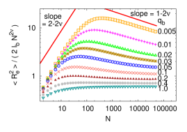
Figure 5: Rescaled mean square end-to-end distance $\langle R_{e}^{2}\rangle/(2\ell_{b}N^{2\nu})$ plotted against the chain length $N$ for semiflexible chains with $\ell_{b}=1$ and various values of $q_{b}$ on a log-log scale. Here $\nu\approx 0.588$ is the Flory exponent for SAWs in $d=3$. Adapted from Ref. WLC3d .

Based on a Flory-like treatment Flory ; Netz , for a chain with $n$ units of the Kuhn length $\ell_{K}$, and diameter $d$ randomly linked together such that the contour length $L=N\ell_{b}=n\ell_{K}$ (there are $(N+1)$ monomers in the chain and connected by the bond length $\ell_{b}$), the effective free energy of such a semiflexible chain contains two terms as follows,

$$\Delta F\approx R_{e}^{2}/(\ell_{K}L)+v_{2}R_{e}^{3}\left[(L/\ell_{K})/R_{e}^{3}\right]^{2}\;.$$ (23)

The first term is the elastic energy which is obtained by treating the chain as a free Gaussian chain, hence one can immediately write down the probability of the end-to-end distance $R_{e}$ which agrees with the Gaussian distribution. Therefore, the elastic energy is simply the logarithm of this distribution. The second term is the repulsive energy due to pairwise contacts where the second virial coefficient $v_{2}=\ell_{K}^{2}d$, the density of monomers $\rho=n/R_{e}^{3}=LR_{e}^{3}/\ell_{K}$ and the volume $V=R_{e}^{3}$. Minimizing $\Delta F$ with respect to $R_{e}$, one obtains the Flory-type result for self-avoiding walks as $L\rightarrow\infty$ $(N\rightarrow\infty)$

$$R_{e}\approx(v_{2}/\ell_{K})^{1/5}L^{3/5}=(\ell_{K}d)^{1/5}(N\ell_{b})^{3/5}\;.$$ (24)

The minimum contour length $L$ where the exclusive volume is effective, i.e. the second term in (23) is negligible in comparison with the first one if $N<N^{*}$, and using the scaling law of the square for the end-to-end distance of a Gaussian chain, $R_{e}^{2}=\ell_{K}L=\ell_{K}\ell_{b}N$, the upper bound of the chain length for describing the Gaussian chain is obtained with

$$N^{*}=\ell_{K}^{3}/(\ell_{b}d^{2})\;.$$ (25)

As $L\leq\ell_{K}$, the chain shows a rod-like behavior, the lower bound of the chain length for the Gaussian chain is given by $\ell_{k}/\ell_{b}$. Therefore, the intermediate Gaussian behavior should only exist for

$$\ell_{k}/\ell_{b}\leq N\leq N^{*}\;.$$ (26)

For a linear semiflexible polymer chain ($d=\ell_{b}$) under good solvent conditions, one would expect to observe both a crossover from rigid rod-like behavior to almost Gaussian random coils, then a crossover to self-avoiding walks when the chain stiffness varies.

In order to verify the prediction, it requires an efficient algorithm to generate sufficient samples for very long semiflexible chains since the results should cover the linear length scales in the three different regimes. PERM was first applied to this in WLC3d . The model described below had indeed been studied by means of PERM already in Theta-WLC , where however most emphasis was put on the question whether the collapse transition changes from second to first order as the stiffness is increased. This was predicted by mean field theories Doniach . The simulations in Theta-WLC supported the prediction, but were dangerously close to the significance limit discussed in Sect. 2.

The above scaling relations for chains without self attraction were studied in WLC3d . Semiflexible polymers were there modelled by SAWs on the simple cubic lattice, with a bending energy $\epsilon_{b}(1-\cos\theta)$. Here $\theta$ is the angle between the new and the previous bonds (only $\theta=0$ and $\theta=\pm\pi/2$ are possible on a simple cubic lattice). The partition function of the SAWs of $N$ steps with $N_{\rm bend}$ local bends (where $\theta=\pm\pi/2$) is

$$Z_{N,N_{\rm bend}}(q_{b})=\sum_{\rm config.}C(N,N_{\rm bend})q_{b}^{N_{\rm bend}}$$ (27)

where $q_{b}=\exp(−\beta\epsilon_{b})$ is the appropriate Boltzmann factor ($q_{b}=1$ for ordinary SAW’s), and $C(N,N_{\rm bend})$ is the total number of chain configurations containing $(N+1)$ monomers and $N_{\rm bend}$ local bends.

In the simulation, the walk of length $n-1$ at the $n^{\rm th}$ step can be guided to either walk straight ahead in any direction, or make an $L$-turn. Of course, it is only allowed to walk to the free nearest neighbor sites of the $n^{\rm th}$ monomer. The ratio of probabilities between the former case and the latter case is chosen as $1/q_{b}$. Since the stiffness of the chain is controlled by $q_{b}$, we give less probability to make an $L$-turn as $q_{b}$ becomes smaller which corresponds to the case that the chain is stiffer. Results of the rescaled mean square end-to-end distance $\langle R_{e}^{2}\rangle/(2\ell_{b}N^{2\nu})$ plotted against the chain length $N$ up to $N=50000$ for $0.005\leq q_{b}\leq 1.0$ are shown in Fig. 5. For stiffer chains, namely for smaller values of $q_{b}$, we do see a rod-like regime at the beginning for not very long chains then a cross-over to a Gaussian regime, and then finally the excluded volume effect becomes more important for very long chains, and a horizontal plateau is developed. For very small $q_{b}$, although the maximum chain length is up to 50000, it does still not yet reach the SAW regime. However, this is the first time that one can give evidence for the existence of the intermediate Gaussian coil regime (26) by using computer simulations.

VII Polymers in Confining Geometries

VII.1 Polymers Confined between Two Parallel Hard Walls

It is a challenge to verify the theoretical scaling predictions for single polymer chains of length $N$ confined between two parallel hard walls with distance $D$ away from each other (Fig. 6) due to the difficulty of producing long polymer chains by MC simulations and the existence of very large finite-size corrections. For unconstrained SAWs, it is well know that the asymptotic scaling behavior is reached rather slowly with correction terms decreasing only as $N^{-0.5}$ LiMadrasSokal ; Belohorec ; GJPA97 . Therefore, in addition to SAWs, we studied also the Domb-Joyce (DJ) model DJmodel with $v=0.6$ (where convergence to asymptotia is much faster Belohorec ; GJPA97 ).

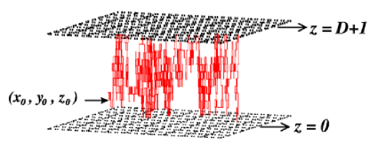
Figure 6: Schematic drawing of a polymer chain confined between two walls located at $z=0$ and $z=D+1$. For our simulations, chains are grown from the starting point $(x_{0},y_{0},z_{0})$. Here $x_{0}$ and $y_{0}$ are fixed but $z_{0}=1,2,\ldots,D$.

In the DJ model, polymers are described by lattice walks where monomers sit at sites, connected by bonds of length one, and multiple visits to the same site are allowed, (i.e. the polymer chain is allowed to cross itself), but the weight is punished by a repulsive energy $\epsilon>0$ for any pair of monomers occupying the same site. Each pair contributes a Boltzmann factor $v=\exp(-\beta\epsilon)$ to the partition sum. Thus, the partition sum of a linear chain consisting of $N+1$ monomers is given by

$$Z_{N}(v)=\sum_{\rm configs.}v^{m}\;,$$ (28)

where the sum extends over all random walk (RW) configurations with $N$ steps, $0\leq v\leq 1$, and $m$ is the total number of monomer pairs occupying a common site, $m=\sum_{i<j}\delta_{{\bf x}_{i}{\bf x}_{j}}$ (${\bf x}_{i}$ denotes the position of the monomer $i$). For $v=1$, it corresponds to the ordinary RW. For $v=0$ it is just the SAW model. In the thermodynamic limit where $N\rightarrow\infty$, the DJ model is in the same universality class of SAW for all $v<1$. There is a “magic” value of the interaction strength $v=v^{*}\cong 0.6$ where corrections to scaling are minimal and asymptotic scaling is reached fastest Belohorec ; GJPA97 . In the renormalization group language, the flow speed of the effective Hamiltonian approaching its fixed point depends on $v$. Moreover, it is approached from opposite sides when $v<v^{*}$ and when $v>v^{*}$, with $v^{*}\cong 0.6$.

There exist important theoretical predictions for the monomer density profile $\rho(z)$ and the end monomer density profile $\rho_{e}(z)$ near the wall given by Eisenriegler et al. Eisenriegler ; Eisenriegler2 as follows:

$$\rho(z)\sim z^{1/\nu_{3}}$$ (29)

and

$$\rho_{\rm end}(z)\sim z^{(\gamma-\gamma^{(1)})/\nu}\sim z^{0.814(6)}$$ (30)

where $z$ is the distance from the wall and $\gamma^{(1)}$ is the entropic exponent for 3D SAW with one end grafted on an impenetrable wall. One should also expect that the density near the walls is proportional to the force per monomer $f$. Indeed it was shown by Eisenriegler Eisenriegler that

$$\lim_{z\rightarrow 0}k\frac{\rho(z)}{z^{1/\nu_{3}}}=B\frac{f}{k_{B}T}=B{a\over\nu_{3}\mu_{\infty}}\;D^{-1-1/\nu_{3}}$$ (31)

with $B$ being a universal amplitude ratio. For ideal chains one has $B=2$, while for chains with excluded volume in $4-\epsilon$ dimensions one has $B\approx 2(1-b_{1}\epsilon)$ with $b_{1}=0.075$ Eisenriegler3 . In three dimensions this gives the prediction $B\approx 1.85$.

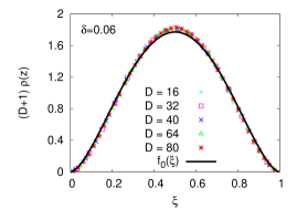
(a)     (b)

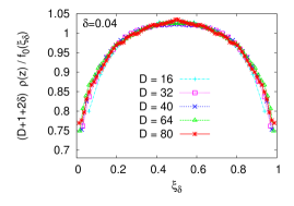
Figure 7: Results of the monomer density profiles $\rho(z)$ obtained for the DJ model. (a) Rescaled values of monomer density $(D+1)\rho(z)$ plotted against $\xi=z/(D+1)$. The function $f_{0}(\xi)=18.74(\xi(1-\xi))^{1/\nu_{3}}$. (b) The same data as in (a), divided by $f_{0}(\xi)$, plotted against a modified scaling variable, $\xi_{\delta}=(z+\delta)/(D+1+2\delta)$ with $\delta=0.04$. The prefactor in (31) for $z=0$ and $z=(D+1)\rightarrow\infty$ is 0.71(3). Adapted from Ref. Slab .

In order to check the above mentioned theoretical predictions, we simulate the SAW model and the DJ model on the simple cubic lattice with the confinement of a slab with width $D$ by using PERM with $6$-step Markovian anticipation. For estimating the monomer density profiles $\rho(z)$ we only count those monomers in the central part of the chain, excluding $10\%$ on either side to avoid errors from the fact that (29) should hold only far away from the chain ends, for monomer indices $n$ satisfying $D^{2}\ll n\ll N-D^{2}$ (we should mention that $N/D^{2}>10$ for all data sets). Results of $\rho(z)$ obtained from the simulations are normalized such that $\sum_{z=1}^{D}\rho(z)=1$. Since we simulate single polymer chains between two walls at $z=0$ and $z=D+1$, we can assume that

$$\rho(z)\approx\frac{1}{D+1}f_{0}\left(\frac{z}{D+1}\right)\enspace{\rm with}\enspace f_{0}(\xi)=A\left[\xi(1-\xi)\right]^{1/\nu_{3}}\;,$$ (32)

where the constant $A=18.74$ is determined by normalization. We plot the rescaled values of the monomer density $(D+1)\rho(z)$ against $\xi$ in Fig. 7(a) for the DJ model. It looks like that the scaling law (29) is satisfied and our data are described by the function $f_{0}(\xi)$ quite well for $z\in[0,D+1]$. But, we actually miss the important information near the two walls in such a plot. A prefactor on the right hand side of (32) is probably not a constant. In order to give a precise estimate of the amplitude $B$ (31) we introduce here an “extrapolation length” $\delta$ as suggested in Milchev so that the scaling variable $\xi$ is replaced by

$$\xi_{\delta}=\frac{z+\delta}{D+1+2\delta}\;.$$ (33)

Using the same data of $\rho(z)$ but divided by $f_{0}(\xi_{\delta})$, the best data collapse shown in Fig. 7(b) is obtained by taking $\delta=0.04$. It leads to $\lim_{z\rightarrow 0,D\rightarrow\infty}D^{1+1/\nu_{3}}z^{-1/\nu_{3}}\rho(z)/A=0.71(3)$. Since the extrapolation length $\delta=0.04$ for the DJ model is much smaller than $\delta=0.15$ for SAWs {see Fig. 7 in Ref. Slab }, it gives a first indication that corrections to scaling are indeed smaller in the DJ model. Using (31), it gives $B=1.70\pm 0.08$. This is only $2$ standard deviations away from the renormalization group expansion prediction or $\epsilon_{c}=4-d$ expansion prediction $B=1.85$ of Eisenriegler Eisenriegler , which we consider as good agreement.

VII.2 Escape Transition of a Polymer Chain from a Nanotube

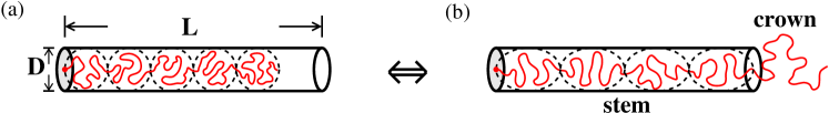
Figure 8: Schematic drawings of a flexible polymer chain of length $N$ grafted to the inner wall of a tube of length $L$ and diameter $D$ at the transition point. (a) As the chain is fully confined in the tube (in an imprisoned state), it forms a sequence of $n_{b}=ND^{-1/\nu}$ blobs in a cigar-like shape, here $\nu=\nu_{3}$ is the Flory exponent in $d=3$. (b) As one part of the chain escapes from the tube (in an escaped state), it forms a flower-like configuration which consists of a “stem” containing $N_{\rm tr}$ monomers and a “crown” containing $N-N_{\rm tr}$ monomers.

The confinement or escape problem of polymer chains in cylindrical tubes of finite length has the merit that it is potentially very relevant to experiments and applications such as the problem of polymer translocation through pores in membranes and the study of DNA confined in artificial nanochannels Salman ; Meller ; Kasianowicz . The following treatment is based on Esc2d ; Esc3d-MAC ; Esc3d-PRE .

Considering a polymer chain of length $N$ with one end grafted to the inner wall of a cylindrical nanotube with finite length $L$ and diameter $D$ under good solvent conditions, the chain configuration is compressed uniformly as $D$ decreases or $N$ increases, but $L$ is fixed. Beyond a certain compression force, the chain configuration changes abruptly from a homogeneously stretched and confined state (imprisoned state) to an inhomogeneous state (escaped state) where polymer chains form a flower-like configuration with one stem confined in the tube and a coiled crown outside the tube (see Fig, 8). This abrupt change implies a first order transition. Since the theory based on the blob picture failed to predict the transition from a homogeneous state to an inhomogeneous state, the Landau theory approach is used for describing such a first order transition including the metastable states. In the Landau theory approach, all configurations are subdivided into subsets associated with a given value of an appropriately chosen order parameter $s$ that allows to distinguish between different states or phases. The full partition function of the system is therefore obtained by integrating over the order parameter:

$$Z=\exp(-F)=\int ds\exp[-\Phi(s)]\;,$$ (34)

where $\Phi(s)$ is the free energy of a given set, and is therefore a function of the order parameter. Here the order parameter $s$ is defined by the stretching degree, i.e. the ratio between the end-to-end distance of monomer segments which are still confined in the tube, $R_{\rm imp}$, and the number of monomers confined in the tube, $N_{\rm imp}$. As shown in Fig. 9, we see that near the transition point the Landau free energy function has two minima, the lower minimum is associated with the thermodynamically stable state, which corresponds to the equilibrium free energy (either $F_{\rm imp}$ or $F_{\rm esc}$) of the system, while the other minimum corresponds to the metastable state Esc3d-MAC ; Esc3d-PRE . At the transition point, both minima are of equal depth.

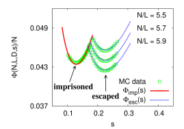
Figure 9: The Landau free energy per monomer, $\Phi(N,L,D,s)/N$ plotted against the order parameter $s$ near the transition point for the tube of length $L=1600$ and diameter $D=17$.

In our simulations, we describe the grafted single polymer chain confined in a tube by SAWs of $N$ steps on a simple cubic lattice with cylindrical confinement $\{0\leq x\leq L,\,y^{2}+z^{2}=D^{2}/4\}$, and the first monomer is attached to the center of the inner wall of the tube. Taking the advantage of PERM that the associated weight of each generated configuration is exactly known, we introduce a new strategy in order to obtain sufficient samplings of the flower-like configurations in the phase space as follows: We first apply a constant force along the tube to pull the free end of a grafted chain outward to the open end of the tube as long as the chain is still confined in a tube, and release the chain once one part of monomer segments of it is outside the tube. Varying the strength of the force, we obtain flower-like configurations containing stems with various stretching degree of monomer segments which are still confined in a tube if the length $N$ is long enough. The contributions for the escaped states are therefore given by properly reweighting these configurations to the situation where no extra force is applied. This is done by using biased SAWs (BSAWs) on a simple cubic lattice with finite cylindrical geometry confinement, similar to the model in (16), but we use here $q=1$ to describe the good solvent condition.

With PERM, the total weight of a BSAW of $N$ steps ($N+1$ monomers) is $W_{b}(N,L,D)=\Pi_{n=0}^{N}w_{n}$ with $w_{n}=b^{(x_{n+1}-x_{n})}/p_{n}$ for $n\geq 1$ and $w_{0}(N,L,D)=1$. $p_{n}$ is chosen as in (18). The estimate of the partition sum is given by

$$\hat{Z}_{b}(N,L,D)=\frac{1}{M_{b}}\sum_{{\rm configs.}\in{\cal C}_{b}}W_{b}({\cal C}_{b})\,$$ (35)

where a set of configurations is denoted by ${\cal C}_{b}$. Thus, each configuration of BSAWs with the stretching factor $b_{k}$ contributes a weight $W^{(k)}(N,L,D)$ for a BSAW of $N$ steps with $b=1$ confined in a finite tube of length $L$ and diameter $D$:

$$W^{(k)}(N,L,D)=\left\{\begin{array}[]{ll}W_{b_{k}}(N,L,D)/b_{k}^{x_{N+1}-x_{1}}\;,&x_{N}\leq L\\ W_{b_{k}}(N,L,D)/b_{k}^{L}\;,&x_{N}>L\end{array}\right.\;,$$ (36)

where index $k$ labels runs with different values of the stretching factor $b$. Combining data runs with different values of $b$, the final estimate of the partition sum is

$$Z(N,L,D)=\frac{1}{M}\sum_{k}\sum_{configs.\in{\cal C}_{b_{k}}}W^{(k)}(N,L,D)$$ (37)

here $M$ is the total number of trial configurations.

The distribution of the order parameter, $P(N,L,D,s)\propto H(N,L,D,s)$, is obtained by accumulating the histograms $H(N,L,D,s)$ of $s$, where $H(N,L,D,s)$ is given by,

$$\begin{array}[]{lll}H(N,L,D,s)&=&\frac{1}{M}\sum_{k}H^{(k)}(N,L,D,s)\\ &=&\frac{1}{M}\sum_{k}\sum_{configs.}\in{\cal C}_{b_{k}}W^{(k)}(N,L,D,s^{\prime})\delta_{s,s^{\prime}}\end{array}$$

and the partition sum of polymer chains confined in a finite tube can be written as

$$Z(N,L,D)=\sum_{s}H(N,L,D,s)$$ (38)

in accordance with (37). Thus, one can also double check the results of the partition sum.

The Landau free energy $\Phi(N,L,D,s)$ here is the excess free energy related to the polymer chains with one end tethered to an impenetrable flat surface, i.e. $\phi(N,L,D,s)=-\ln\left[P(N,L,D,s)/Z_{1}(N)\right]$ ($Z_{1}(N)\sim\mu^{N}N^{\gamma_{1}-1}$ Graf-G05 ). Results shown in Fig. 9 are for $L=1600$, $D=17$, and for $N/L=5.5$, $5.7$, $5.9$. This shows that the information about metastable states can also be extracted from the simulations with PERM.

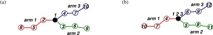
Figure 10: Schematic drawings of a star polymer consisting of three arms $(f=3)$ of length $N=3$ each. The center is singly occupied in (a) and $f$-folded occupied in (b). Those numbers show the order of monomers which is added into the star polymer by using a chain growth algorithm.

VIII PERM for Branched Polymers with Fixed Tree Topologies

In this section we shall discuss two types of branched tree-like polymers: Star polymers (where all branches emanate from one single point) and “bottle brushes” where side chains of common lengths are attached to a backbone at regularly spaced points.

To be concrete, let us consider the simplest case of a branched polymer, a star polymer where $f$ arms are grafted to a single branch point, and all arms have the same length $N$.

As a linear chain is built by using PERM, at each step one monomer is added to the built chain until the chain has reached its maximum length $N$ or it has been killed in between. For growing a star polymer we have to be aware that not only the interactions between monomers in the same arm have to be considered but also the interactions between monomers on different arms have to be taken into account. If one arm is grown entirely before the next arm is started, it will lead to a completely “wrong” direction of generating the configurations of a star. However, it is straightforward to modify the basic PERM algorithm such that all $f$ arms of a star polymer are grown simultaneously Star1 ; Star2 . The multi-arm method is explained as follows:

• A star polymer is grown from its branching point (center).

• $f$ growth sites $\{{\bf x}_{1},\ldots{\bf x}_{f}\}$ are considered at the same time. A monomer is added to each arm step by step until all arms have the same length, then the next round of monomers is added. As all the monomers in a star are numbered, it is similar as growing one linear chain from the $1^{\rm st}$ monomer to the $N_{\rm max}^{\rm th}$ monomer (see Fig. 10). $N_{\rm max}=Nf+1$ if the center is singly occupied or $N_{\rm max}=Nf+f$ if the center is $f$-folded occupied.

• A bias is given to guide the growth of arms into outward direction with higher probability. The strength of this bias is adjusted in the way that it increases with $f$ but decreases as the length of arms becomes longer since there is more space in a dilute solvent for adding the next monomer. For example, we can choose the bias as a function of $n$, $g(n)$, for $n\geq 0$,

  $$g(n)=\left\{\begin{array}[]{ll}(n+4.0)/(n+1.3)\;,&\enspace{\rm outward\,direction}\\ (n+0.6)/(n+3.9)\;,&\enspace{\rm otherwise}\end{array}\right.\;.$$ (39)

  However, the strength of this bias can be adjusted by trial and error.

• The population control (pruning/cloning) is done in the same way as explained in Sect. II that at the step $n$, two thresholds $W_{n}^{+}$ and $W_{n}^{-}$ are proportional to the current estimate weight $\hat{Z}_{n}$, e.g., $W_{n}^{+}=3\hat{Z}_{n}$ and $W_{n}^{-}=0.5\hat{Z}_{n}$.

VIII.1 Star Polymers

For single star polymers composed of $f$ arms of length $N$ each in a good solvent, the partition sum and the rms center-to-end distance scale as follows:

$$Z^{(1)}_{N,f}\sim\mu_{\infty}^{-fN}N^{\gamma_{f}-1}$$ (40)

and

$$R^{2}_{N,f}\approx A_{f}N^{2\nu}$$ (41)

where the critical fugacity $\mu_{\infty}$ and the Flory exponent $\nu$ are the same for all topologies but the entropic exponent $\gamma_{f}$ depends on each topology Duplantier . In two dimensions, $\gamma_{f}$ can be calculated exactly by using conformal invariance Duplantier , but there are no exact results for the $f$-dependent power law for $\gamma_{f}$, and also not for the swelling factor $A_{f}$. Therefore, computer simulations are needed for a deep understanding of star polymers. Due to the difficulty of simulating the star polymers with many arms $f$ and of long arm length $N$ by both MC simulations Barrett ; Batoulis ; Shida ; Dicecca ; Ohno ; Zifferer and molecular dynamics Grest ; Grest94 , and because of the lack of precise estimates of the exponents given in (40) and (41), PERM with multi-arm growth method as explained above was developed Star1 . With this algorithm, high statistics simulations are obtained for star polymer with arm number up to $f=80$ and arm length up to $N=4000$ for small values of $f$.

For our simulations of single star polymers in a good solvent, we use the Domb-Joyce model with the interaction strength $v^{*}=0.6$ on the simple cubic lattice (see Sect. VII.1). It allows us to attach a larger number of arms to a point-like center of stars, and thus additional considerations of the corrections to scaling terms when a finite size core is used are avoided. Two variants for studying star polymers are used in our simulations. In one variant the center is occupied by one monomer, and in the other variant the center is occupied by $f$ monomers as shown in Fig. 10. Since the partition sum is estimated directly by PERM, the exponents $\gamma_{f}$ can also be determined easily according to (40).

In Fig. 11, we present results of $\gamma_{f}$ from our simulations and from previous studies Batoulis ; Shida ; Schaefer92 for comparison. The theoretical prediction for the scaling law of $\gamma_{f}$ for large $f$ by the cone approximation Ohno ; Witten is

$$\gamma_{f}-1\sim f^{-3/2}$$ (42)

For small $f$, our results are in good agreement with the previous studies. For large $f$ the best fit with a power law $\gamma_{f}-1\sim-(f-1.5)^{z}$ would be obtained with $z\approx 1.68$, which is not too far off the theoretical prediction (42) but the prediction is also not exact.

(a)

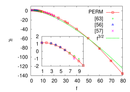
Figure 11: Exponents $\gamma_{f}$ plotted against $f$. The full line is just a polygon connecting the points, and the dashed line is a fit with the large-$f$ behavior as predicted by the cone approximation (42). Results obtained in Ref. Batoulis ; Shida ; Schaefer92 are shown for comparison. In the inset, we show those results for small $f$. Adapted from Ref. Star1 .

After we have obtained quite reliable estimates of $\mu_{\infty}$, $\nu$, and $\gamma_{f}$ for single star polymer in a good solvent, we extend our study to a more complicated system where two star polymers interact with each other Star2 by using the same model and the same algorithm. It is well understood that interactions between both linear and branched polymers are soft in the sense that they can penetrate each other and the effective potential is a rather smooth function of their distance. For star polymers, there are some contradictions between results in the literatures. Is the potential between two central monomers at large distance a Gaussian potential or has it a Yukawa tail? Since we were able to simulate star polymers up to $f=80$ arms, we expected that we would give a clear answer. This was the main motivation to study the effective potential between two star polymers Star2 .

Witten and Pincus Witten point out that the scaling of the partition sum of a star with $f$ arms and arm length $N$ each (40), together with the assumption that $Z^{(2)}_{N,f}(r)/\left[Z_{N,f}^{(1)}\right]^{2}$ is a function of $x\equiv r/R_{g}$ only for any fixed $f$, i.e.

$$\frac{Z^{(2)}_{N,f}(r)}{\left[Z_{N,f}^{(1)}\right]^{2}}=\psi_{f}(r/R_{g})\;,$$ (43)

implies that

$$V(r)\approx V_{\rm WP}(r)\equiv b_{f}\ln(a_{f}R_{g}/r)$$ (44)

where $r$ is the distance between the two central monomers, and

$$b_{f}=(2\gamma_{f}-\gamma_{2f}-1)/\nu\qquad{\rm for}\enspace 1\ll r\ll R_{g}\;.$$ (45)

According to our results shown in Fig. 11, instead of the scaling $b_{f}\sim f^{3/2}$, a power law gives $b_{f}\approx 0.27f^{1.58}$. However, both $a_{f}$ and $b_{f}$ should be universal and should not depend on the specific microscopic realization.

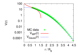
(a)     (b)

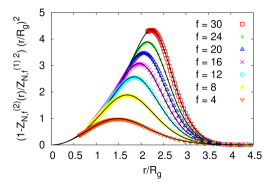
Figure 12: (a) The effective potential $V(r)$ for $f=18$, plotted against $R_{g}$ in a semi-log scale. The solid curve shows (44), and the dotted curve is a Gaussian. (b) Rescaled radial Mayer functions against $r/R_{g}$ for several values of $f$. Curves are obtained from (48), with fitted parameters $a_{f}$, $c_{f}$, $d_{f}$ and $\tau_{f}$. Adapted from Ref. Star2

There are two methods for estimating $Z^{(2)}(r)$ in our simulations:

• Two independent star polymers are grown simultaneously, and $Z^{(2)}(r)$ is computed by counting their overlaps at different distance $r$. Here $Z^{(2)}(r)$ and $Z^{(1)}(r)$ are estimated in the same run, which gives rather accurate results for the potential $V(r)$ for very large distances $r$ and large $N$. For small distances $r$, the ratio $Z^{(2)}(r)/\left[Z^{(1)}(r)\right]^{2}$ would be indistinguishable from zero.

• Two star polymers are grown at fixed distance $r$ with the mutual interactions taken into account during the growth. This allows us to measure $Z^{(2)}(r)$ down to very small distances $r$ and large $N$. For large distances $r$, it gives very bad results of the potential $V(r)$ since it is obtained by subtracting the (nearly equal) free energies obtained in two different runs.

For the data analysis, we use the data either from the first method or the second method, or use the combination from both.

We present the effective potential $V(r)$ between two star polymers of $f=18$ arms in Fig. 12(a). For $r\ll R_{g}$, $V(r)$ follows the prediction given in (44), which is shown by the solid curve. For $r\gg R_{g}$ the MC data can be approximated by a parabola, i.e. $V(r)$ is roughly Gaussian

$$V(r)\approx V_{\rm Gauss}(r)\equiv c_{f}e^{d_{f}r^{2}/R_{g}^{2}}\;.$$ (46)

Here we conjecture that $c_{f}$ and $d_{f}$ are universal. In order to describe the effective potential $V(r)$ for the whole region of $r$, we propose that

$$V(r)=\frac{1}{\tau_{f}}\ln\left[e^{\tau_{f}V_{\rm WP}(r)-d_{f}r^{2}/R_{g}^{2}}+e^{\tau_{f}V_{\rm Gauss}(r)}\right]\;,$$ (47)

where $\tau_{f}$ is an additional parameter for every $f$, and $V(r)>0$ for all $r$. As $r\rightarrow\infty$, $V(r)=V_{\rm Gauss}(r)[1+O(r^{-b_{f}})]$ (46), while $V(r)=V_{\rm WP}(r)[1+O(r^{2})]$ (44) as $r\rightarrow 0$. In fig 12(b), we plotted the rescaled radial Mayer function,

$$(r/R_{g}^{2})^{2}f_{M}(r)=(r/R_{g})^{2}(a-\exp[-V(r)])\;,$$ (48)

against the rescaled distance $r/R_{g}$. Our results are in good agreement with the simulations of Rubio but do not agree with the results in Likos .

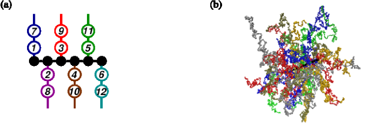
Figure 13: (a) A schematic drawing of growing a bottle-brush polymer step by step. (b) A snapshot of the configurations of bottle-brush polymers consisting of $N_{b}=128$ backbone monomers, $N=2000$ monomers in each side chain, and the grafting density $\sigma=1/4$ under a very good solvent condition generated by PERM.

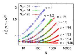
(a)     (b)

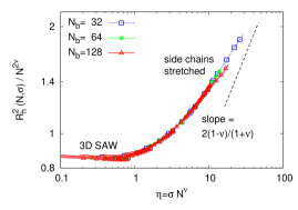
Figure 14: (a) Log-log plot of rescaled mean square height $R^{2}_{h}(N,\sigma)/N^{2\nu}$ versus $N$ (a) and $\eta=\sigma N^{\nu}$ (b) with $\nu\approx 0.588$. Results are obtained for three choices of $N_{b}$ and several choices of the grafting density $\sigma$ as indicated. Those unphysical data ($R_{h}>0.5N_{b}$) due to the artifact of using periodic boundary condition are removed. The slope of the straight line corresponds to the scaling prediction. Adapted from Ref. Brush2 .

VIII.2 Bottle-brush Polymers

The so-called bottle-brush polymer consists of one long molecule serving as a backbone on which many side chains are densely grafted. As the grafting density $\sigma$ increases, the persistence length of the backbone increases. The bottle-brush polymer has the form of a rather stiff cylindrical-like object. If the backbone is very short but side chains are very long, it should behave like a star polymer. If the backbone is very long, the structure becomes more complicated. One would expect that those side chains in the interior of the bottle-brush are all stretched and show the same behavior, but those at the two ends behave as a star. In order to understand the structure of bottle-brush polymers and check the scaling behavior of long side chains in comparison with theoretical predictions Brush2 , we focus here the bottle-brush polymers of a rigid backbone and flexible side chains.

For our simulations, we use a simple coarse-grained model. The backbone is treated as a completely rigid rod, and side chains are described by SAWs with nearest neighbor non-bonded attractive interactions between the same type of monomers and repulsive interactions between the different type of monomers. A general formula for the partition function for bottle-brush polymers consisting of one or two chemically different monomers is therefore given by

$$Z=\sum_{\rm config.}q^{m_{AA}+m_{BB}}q_{AB}^{m_{AB}}$$ (49)

where $q=\exp(-\beta\epsilon)$ (we assume that the attractive interaction $\epsilon_{AA}=\epsilon_{BB}=\epsilon$), $q_{AB}=\exp(-\beta\epsilon_{AB})$ ($\epsilon_{AB}$ is the repulsive interaction between monomer $A$ and monomer $B$), and $m_{AA}$, $m_{BB}$, $m_{AB}$ are the numbers of non-bonded occupied nearest neighbor monomer pairs $AA$, $BB$ and $AB$, respectively. For $q=1$, all side chains behave as SAWs. For $q<q_{\Theta}$ it corresponds to the good solvent condition, where $q_{\Theta}=\exp(-\epsilon/k_{B}T_{\Theta})\approx 1.3087$ at the $\Theta$ point Grassberger97 . For $q>q_{\Theta}$, it corresponds to the poor solvent condition. As $q_{AB}=0$, it corresponds to a very strong repulsion between $A$ and $B$, while for $q_{AB}=q$ the chemical incompatibility vanishes {recall that deGennes $\chi_{AB}\propto\epsilon_{AB}-(\epsilon_{AA}+\epsilon_{BB})/2\}$. The grafting density $\sigma$ is defined by $\sigma=n_{c}/N_{b}$ where $n_{c}$ is the number of side chains and $N_{b}$ is the number of monomers in a backbone. Here only the results of bottle-brush polymers consisting of one kind of monomers under a very good solvent condition are presented in order to show the performance of the algorithm. Other applications can be found in Brush2 ; Brush1 ; Brush3 ; Brush4 .

We extend the algorithm for simulating star polymers to bottle-brush polymers. As shown in Fig. 13(a), a bottle-brush polymer is built by adding one monomer to each side chain at each step until all side chains have the same number of monomers. Then we start to add the second run of monomers, i.e, all side chains are grown simultaneously. The bias of growing side chains was used by giving higher probabilities in the direction where there are more free next neighbor sites and in the outward directions perpendicular to the backbone, where the second part of bias decreases with the length of side chains and increases with the grafting density. A typical configuration of bottle-brush polymers consisting of $N_{b}=128$ backbone monomers, $N=2000$ side chain monomers, and with grafting density $\sigma=1/4$ under a good solvent condition is shown in Fig. 13(b) where the total number of monomers is $N_{\rm tot}=128+2000\times 32=64128$ monomers.

For checking the scaling law of side chains, we introduce the periodic boundary condition along the direction of the backbone ($+z$-direction) to avoid end effects associated with a finite backbone length. The square of the average height of a bottle-brush polymer, $R_{h}^{2}(N,\sigma)=\langle R_{ex}^{2}(N,\sigma)+R_{ey}^{2}(N,\sigma)\rangle$ is estimated by taking the average of the mean square backbone-to-end distance in the radial direction for all side chains. In Fig. 14(a) we plot $R_{h}^{2}(N,\sigma)$ divided by $N^{2\nu}$ versus $N$ for $N_{b}=32$, $64$, and $128$, for various values of grafting densities $\sigma$. The value of $\nu$ is given by the best estimate for 3d SAW by PERM Star1 . We see that those curves of the same grafting density $\sigma$ coincide with each other. Increasing the grafting density $\sigma$, it enhances the stretching of side chains. As $\sigma\rightarrow 0$, we should expect a mushroom regime where no interaction between side chains appears. As $\sigma$ is very high, the scaling prediction obtained by extending the Daoud-Cotton Daoud “blob picture” Wang ; Ligoure ; Sevick ; Grest95 from star polymers to bottle-brush polymers is $R_{h}^{2}(N,\sigma)\propto\sigma^{2(1-\nu)/(1+\nu)}N^{4\nu/(1+\nu)}$. Thus, we can give the cross-over scaling ansatz as follows for $N\rightarrow\infty$,

$$R^{2}_{h}(N,\sigma)=N^{2\nu}\tilde{R}^{2}(\eta)$$ (50)

with

$$\tilde{R}^{2}(\eta)=\left\{\begin{array}[]{ll}1\enspace\;,&\eta\rightarrow 0\\ \eta^{2(1-\nu)/(1+\nu)}\enspace\;,&\eta\rightarrow\infty\end{array}\right.$$ (51)

where $\eta=\sigma N^{\nu}$.

After removing those unphysical data due to the artifact of using periodic boundary condition in the regime where $R_{h}(N,\sigma)>N_{b}/2$, we plot the same data of $R_{h}^{2}(N,\sigma)/N^{2\nu}$ but rescaled the x-axis from $N$ to $\eta=\sigma N^{\nu}$ according to the scaling law (50). We see the nice data collapse in Fig. 14(b). In this log-log plot, the straight line gives the asymptotic behaviors of the scaling prediction (50) for very large $\eta$. As $\eta$ increases, we see a cross-over from a 3D SAWs to a stretched side chain regime but only rather weak stretching of side chains is realized, which is different from the scaling prediction. However, this is the first time one can see the cross-over behavior by computer simulations. This cross-over regime is far from reachable by experiments.

IX PERM with Cluster Growth Method

It is generally believed that lattice animals, lattice trees, and subcritical percolation are good models for studying randomly branched polymers and they are in the same universality class. There exist several efficient algorithms, e.g., Leath algorithm Leath , Swendsen-Wang algorithm Swendsen , etc. for studying the growth of percolation clusters near the critical point, but they all become inefficient far below it, because the chance for growing a large subcritical cluster by a straightforward algorithm decreases rapidly with $N$. Obviously we need some sort of cloning, and since this will probably lead also to fluctuating weights, one might need some pruning.

Cloning and pruning needs first some estimate for the weight of a cluster that is still growing. Moreover, it will turn out that growing clusters can have, depending on their detailed configurations, very different probabilities to grow further. Thus, in addition to a weight we might to need also a “fitness” that should depend on the weight but is not entirely determined by it.

In the following discussion the algorithm is explained by considering the relationship between the site percolation and site lattice animals Anim1 .

In any cluster growth algorithm Leath , a finished cluster with $N$ sites and $b$ boundary sites on a lattice is generated with probability

$$P_{Nb}=p^{N}(1-p)^{b}\;,$$ (52)

if each lattice site is occupied with the probability $p$. By definition of lattice animals all the clusters of same size $N$ carry the same weight. Since the obtained percolation cluster is biased by the probability $P_{Nb}$, its contribution to the animal ensemble is corrected by a factor $1/P_{Nb}$. Taking an average over the percolation ensemble, the partition sum of lattice animals consisting of $N$ sites is given by

$$Z_{N}=\langle\frac{1}{P_{Nb}}\rangle=p^{-N}\langle(1-p)^{-b}\rangle$$ (53)

As shown in Fig. 15, now we consider a cluster with $N$ sites, $g$ growth sites and $b$ boundary sites. At each of the growth sites the cluster can either grow further, or it can stop growing with the probability $1-p$. Thus, this still growing cluster gives a weight to a percolation cluster with $N$ sites and $(b+g)$ boundary sites as $p^{N}(1-p)^{b+g}/\left[p^{N}(1-p)^{b}\right]=(1-p)^{g}$. Taking an average over all clusters, we have

$$Z_{N}=\langle\frac{(1-p)^{g}}{p^{N}(1-p)^{b+g}}\rangle=p^{-N}\langle(1-p)^{-b}\rangle\;.$$ (54)

This is the same formula as given by (53), but note that now we have included also those clusters which are still growing.

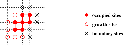
Figure 15: A still growing cluster with $N=7$ sites, $b=6$ boundary sites and $g=6$ growth sites on a square lattice.

Figure 16: Growing clusters generated in the (a) depth-first and (b) breadth-first implementations. In both cases, $p=p_{c}=0.5927$ and $N=4000$. Occupied sites and growth sites are depicted by small red points and big black points, respectively. Adapted from Ref. Anim1 .

Let us first point out this new variant of PERM:

• The percolation cluster growth algorithm with storing the growth sites into a queue in a first-in first-out list (the scheme of breadth-first) is used.

• The population control is done by introducing a fitness function

  $$f_{n}=W_{n}/(1-p)^{\alpha g}=p^{-n}(1-p)^{-b-\alpha g}$$ (55)

  with a parameter $\alpha$ to be determined empirically, and used

  $$f_{n}>c_{+}\langle f_{n}\rangle,\qquad f_{n}<c_{-}\langle f_{n}\rangle$$ (56)

  as criteria for cloning and pruning.

• The depth-first implementation in PERM is still used here. Namely, at each time one deals with only a single configuration of a cluster until a cluster has been grown either to the end of the maximum size $N$ or has been killed in between, and handles the copies by recursion.

• The optimal value of the probability $p$ is $p<p_{c}$, and $p\rightarrow p_{c}$ as $N\rightarrow\infty$.

This algorithm was developed more or less by trial and error, guided by the following considerations:

We first test the two common ways for growing the percolation clusters. (a) Depth-first: growth sites are written into a first-in last out list (a stack). (b) Breadth-first: growth sites are written into a first-in first-out list (a queue). In order to avoid the mix up with the depth implementation in PERM, we use stack and queue to distinguish these two methods. Two typical 2-$d$ clusters of size $N=4000$ and at the critical point of percolation $p=p_{c}=0.5925$, growing according to these two methods are shown in Fig. 16. At first glance, one would expect that the cluster growing by storing growth sites in a stack might be more efficient than that the growth sites stored in a queue, because the number of growing sites was about 3 times larger than that for the latter case. But the truth is, after a few generations the descendents generated from the former case will die. On the other hand, the fluctuations in the number of growth sites are much bigger in the former case, the weights in (54) will also fluctuate much more, and we expect much worse behavior. This is indeed what we found numerically: Results obtained when using a stack for the growth sites were dramatically worse than results obtained with a queue.

Second, we check whether the efficiency is affected by the chosen order of writing the neighbors of a growth site into the list. Studying the percolation cluster in two dimensions, one can use the preferences east-south-west-north, or east-west-north-south, or a different random sequence at every point. We found no big differences in efficiency.

Third, it would be far from optimal to do the population control as explained in Sect. II, i.e. by using two thresholds $W^{\pm}$ on the current weights $W_{n}\equiv p^{-n}(1-p)^{-b}$. This would strongly favor clusters with few growth sites, since they tend to have larger values of $b$, for the same $n$, and have thus large weights. But such clusters would die soon, and would thus contribute little to the growth of much larger clusters. Therefore a proper fitness function $f_{n}$ is needed.

Finally, we have to decide the optimal values of $p$ empirically. It is clear that we should not use $p>p_{c}$, because it is subcritical percolation that is in the same universality class of lattice animal. One might expect $p\ll p_{c}$ to be optimal because only minimal reweighting is needed for small $p$. This is indeed true for small $N$, but not for large $N$. In order to reach large $N$, it is more important that clusters grown with $p\ll p_{c}$ have to be cloned excessively. otherwise, they would die rapidly in view of their few growth sites. In Fig. 17 we present the errors of free energies $F_{N}=-\ln Z_{N}$ for various values of $p$ in $d=2$ and $d=8$. The statistical errors always eventually decrease as $1/\left[{\rm CPU\,time}\right]^{1/2}$, hence we show there one standard deviation multiplied by $\left[{\rm CPU\,time}\right]^{1/2}$ (measured in seconds), for different values of $p$. Thus, we can compare the accuracy between those runs on different computers. For $d=2$ (Fig. 17(a)), each simulation was done for $N_{\rm max}=4000$ (although we plotted some curves only up to smaller $N$, omitting data which might not have been converged). We see clearly that small values of $p$ are good only for small $N$. As $N$ increases, the best results were obtained for $p\to p_{c}$. The same behavior was observed also in all other dimensions, and also for animals on the bcc and fcc lattices in 3 dimensions (data not shown). In Fig. 17(b), we see the analogous results for $d=8$ and for $N_{\rm max}=8000$, showing the errors are much smaller than those in Fig. 17(a). Indeed, the errors decreased monotonically with $d$, being largest for $d=2$. Using $p$ slightly smaller than $p_{c}$ we can obtain easily very high statistics samples of animals with several thousand sites for dimensions $\geq 2$. Another quantity which can help to check the reliability of our data is the tour weight distribution (see Sect. II). In Fig. 18, we show the two tour weight distributions for two-dimensional animals with 4000 sites, for $p=0.57$ and for $p=0.47$. We see that the simulation with $p=0.57$ is distinctly on the safe side, while that for $p=0.47$ is marginal. In the log-log plot, it is seen that the tail of the distribution $P(\ln{\cal W})$ for $p=0.57$ decays faster than $1/{\cal W}$, thus the product ${\cal W}P(\ln{\cal W})$ has its maximum where the distribution is well sampled.

Error bars quoted in the following on raw data (partition sums, gyration radii, and average numbers of perimeter sites or bonds) are straightforwardly obtained single standard deviations. Their estimate is easy since clusters generated in different tours are independent, and therefore errors can be obtained from the fluctuations of the contributions of entire tours (notice that clusters within one tour are not independent, and estimating errors from their individual values would be wrong).

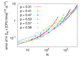
(a)     (b)

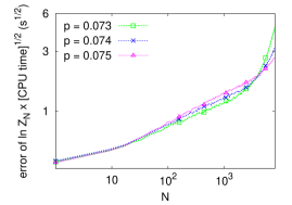
Figure 17: Statistical errors of $\ln Z_{N}$ for lattice animals in $d=2$ (a) and $d=8$ (b) for various values of $p$. To make the different runs comparable, errors are multiplied by the square root of the CPU time measured in seconds. The cluster size $N$ is up to $4000$ in (a) and up to $8000$ in (b). The percolation thresholds are $p_{c}=0.5927$ in $d=2$, and $p_{c}=0.0752$ in $d=8$. Adapted from Ref. Anim1 .

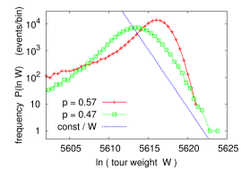
Figure 18: Log-log plot of distributions of tour weights $P(\ln W)$ of $2d$ animals with $N=4000$, for $p=0.57$ and $p=0.47$, together with a straight line representing the function $y=const/W$. Adapted from Ref. Anim1 .

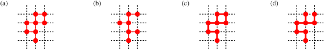
Figure 19: (a) A site animal with $8$ sites. (b) A site tree (“strongly embeddable tree”). (c) A bond animal which is not a tree. (d) A bond tree (“weakly embeddable tree”).

Figure 20: Typical site lattice animals with $N=12000$ on the square lattice in $d=2$ (a), with $N=16000$ on the bcc lattice in $d=3$ (b).

In addition to site animals, this algorithm can also be applied to bond animals and lattice trees for studying randomly branched polymers. A bond animal is a cluster where bonds can be established between neighboring sites (just as in SAWs), and connectivity is defined via these bonds: if there is no path between any two sites consisting entirely of established bonds, these sites are considered as not connected, even if they are nearest neighbors. Different configurations of bonds are considered as different clusters, and clusters with the same number of bonds (irrespective of their number of sites) have the same weight Janse . Weakly embeddable trees are bond animals with tree topology, i.e. the set of weakly embeddable trees is a subset of bond animals, each with the same statistical weight. Strongly embeddable trees are, in contrast, the subset of site animals with tree-like structure. All these definitions are illustrated in Fig. 19.

IX.1 Non-interacting Lattice Animals in the Bulk

The basic problem of lattice animals (site animals) is how to count the number of different animals of $N$ sites precisely, i.e. the estimate of the corresponding partition sum. Two animals are considered as identical if they differ just by a translation, but they considered as different if a rotation or reflection is needed to make them coincide. Two typical site animals consisting of $N=12000$ sites on the square lattice in $d=2$ and with $N=16000$ sites on the body centered cubic (bcc) lattice in $d=3$ are shown in Fig. 20.

In the thermodynamic limit as $N\rightarrow\infty$, the number of animals (i.e. the microcanonical partition sum) should scale as Lubensky

$$Z_{N}\sim\mu^{N}N^{-\theta}(1+b_{z}N^{-\Delta}+\cdots)\;,$$ (57)

and the gyration radius as

$$R_{N}\sim N^{\nu}(a+b_{R}N^{-\Delta}+\cdots)$$ (58)

Here $\mu$ is the growth constant (or inverse critical fugacity), and is not universal, while the Flory exponent $\nu$, the entropic exponent $\theta$, and the correction exponent $\Delta$ Adler should be universal. $b_{z}$ and $b_{R}$ are non-universal amplitudes, and the dots stand for higher order terms in $1/N$.

Results of the partition sum $Z_{N}$ and the mean square end-to-end distance $R^{2}_{N}$ for site lattice animals in $d=2$ are shown in Fig. 21. By taking the predicted value of $\theta=1$ and plotting $\ln Z_{N}-aN+\ln N$ against $N$, we should expect a curve which becomes horizontal for large $N$ by adjusting values of $a=\ln\mu$ suitably. This is indeed seen for the central curve with error bar in the inset of Fig. 21(a), but a precise estimate of $\mu$ is difficult because of corrections to scaling. Considering the first correction term in (57) and (58), the correction exponent $\Delta$, and the estimate of the growth constant $\mu$ and their error bars are all determined by the best straight line as $N^{-\Delta}\rightarrow 0$ in Fig. 21. Our estimate of $a=\ln\mu=1.4018155(30)$ with $\Delta=0.9(1)$ is in perfect agreement with the exact enumeration result Jensen . The Flory exponent $\nu$ is determined by the same way and our estimate $\nu=0.6412(5)$ is also in good agreement with the previous estimate by Monte Carlo simulations You .

(a)     (b)

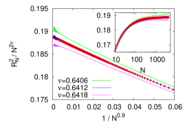
Figure 21: (a) Results of $\ln Z_{N}-aN+\theta\ln N$ plotted against $N^{-\Delta}$, and against $N$ (in the inset), and (b) results of $R^{2}_{N}/N^{2\nu}$ plotted against $N^{-\Delta}$, and against $N$ (in the inset). The best estimates of $a=\ln\mu=1.4018155(30)$, $\nu=0.6412(5)$ and $\Delta=0.9(1)$ are given by the best straight lines. All data are for site lattice animals in $d=2$. Adapted from Ref. Anim1 .

It is trivial to generalize the algorithm PERM with cluster growth method to lattice animals in higher dimensions $2<d\leq 9$. Using the similar method of data analyses as shown in Fig. 21 for those results obtained in $d=3$ to $d=7$ ($d_{c}=8$ is the upper critical dimension of lattice animals, where large corrections have to be taken into account). The relationship between the entropic exponent $\theta$ and the Flory exponent $\nu$ for the animal problem in $d$ dimensions is predicted by using supersymmetry Parisi ,

$$\theta=(d-2)\nu+1$$ (59)

By plotting our data of the exponent $\nu$ and $(\theta-1)/(d-2)$ against $d$ in Fig. 22, we see that these two curves coincide with each other. It shows that the Parisi-Sourlas prediction (59) is verified.

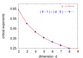
Figure 22: The critical exponents $\nu$ and $(\theta-1)/(d-2)$ against $d$. Adapted from Ref. Anim1 .

IX.2 Lattice Animals Grafted to Surfaces

For a-thermal walls (which represent only a geometric barrier, without any other interactions) the leading behavior for $N\to\infty$ does not involve any new critical exponent Anim1 . This is no longer true, however, if the wall is attractive. In that case we expect a phase transition at a critical attractive energy beyond which the animal gets adsorbed to the surface, similar to the adsorption transition observed also for linear polymers Graf-G05 .

As in that problem, at the transition point there are new critical exponents. More precisely, the Flory exponent $\nu$ is the same as for non-grafted animals, but the entropic exponent $\theta$ is changed Anim1 . Since this exponent could not be measured by any previous simulation algorithm and since there exits no field-theoretic predictions for it, there exist no literature values to compare to our measurements. This is different for a second new exponent specific for the transition point, the cross-over exponent $\phi$. If $q$ is the Boltzmann factor for the monomer-wall interaction and $q_{c}$ is its critical value, then the scaling ansatz for the partition sum of a grafted animal near the adsorption transition is

$$Z^{(1)}_{N}(q)\sim\mu(q)^{N}N^{-\theta_{s}}\Psi[(q-q_{c})N^{\phi}].$$ (60)

The most interesting prediction for $\phi$ was that is superuniversal, i.e. its value is independent of the dimension and $\phi=1/2$ for all dimensions Lyssy . While this was verified by the simulations for $d=3,4$ and 5, it was slightly violated (by 5 standard deviations) in $d=2$ Anim1 . Obviously further investigations would be needed to settle this problem.

IX.3 Conformal Invariance and Animals Grafted to Wedges

The critical exponents for animals in $d=2$ dimensions can be calculated exactly, as for many other critical phenomena in $d=2$ dimensions. But while this is due to conformal invariance in these other cases, 2-d animals are not conformally invariant Miller .

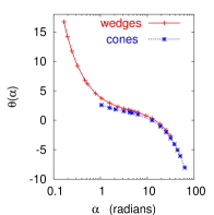
Figure 23: Entropic critical exponents $\theta(\alpha)$ for 2-d lattice animals grafted to the tips of wedges resp. cones with angles $\alpha$. Adapted from Ref. Anim3 .

For conformally invariant problems of cluster growth, the entropic critical exponents of clusters grafted to the tips of wedges and cones (wedges with identified edges) can be calculated exactly for any wedge angle, by mapping the wedge onto the half plane. Due to lack of conformal invariance, this is no longer true for 2-d lattice animals. In Anim3 , the exponents $\theta(\alpha)$ were measured carefully not only for wedges and cones with angles up to $\alpha=2\pi$. By grafting them to branch points of Riemann sheets, angles up to $10\pi$ were studied. Results are shown in Fig. 23. The simulations were made with the hope that someone might produce a fit to these data that could suggest an alternative to conformal invariance. So far this hope has not materialized, in contrast to what happened 111 years ago to some obscure black body radiation data Lummer .

IX.4 Collapsing Lattice Animals and Lattice Trees in $d=2$

A coil-globule transition similar to that for linear polymers is also expected to occur for randomly branched polymers as the solvent quality becomes worse, but the situation is much more complicated. To describe the possible collapse transitions for self-interacting lattice animals, we need two different types of interactions between nearest-neighbor monomer-monomer pairs: (covalent) bonds that are needed for the connectedness of the cluster but that can also form loops when present in excess, and weak interactions between non-bonded pairs (“contacts”). Associated to these are two different control parameters Flesia . The partition sum is therefore written as follows Anim2

$$Z_{N}(y,\tau)=\sum_{b,k}C_{Nbk}y^{b-N+1}\tau^{k}$$ (61)

where $C_{Nbk}$ is just the number of configurations (up to translations and rotations) of connected clusters with $N$ sites, $b$ bonds, and $k$ contacts. $y$ and $\tau$ are fugacities for monomer-monomer bonds and for non-bonded monomer-monomer contacts, respectively. As for unbranched polymers, there is no need to introduce a separate monomer-solvent interaction, since the number $s$ of monomer-solvent contacts is not independent, but is given by

$${\cal N}N=2b+2k+s\;,$$ (62)

where ${\cal N}$ is the lattice coordination number (${\cal N}=2d$ on a simple hypercubic lattice in $d=2$ dimensions). A schematic drawing of an interacting lattice animal is shown in Fig. 24. This model includes the following special cases:

• Unweighted animals: $y=\tau=1$

• Bond percolation: $y=p/(1-p)^{2}$ and $\tau=1/(1-p)$ where $0\leq p\leq 1$. The critical percolation point is at $y=2$ and $\tau=2$ as $p=p_{c}=1/2$.

• Collapsing trees: $y=0$ where $b=N-1$.

• ‘Strongly embeddable’ animals with $\tau=0$, which have no contacts ($k=0$) This model was first studied by Derrida and Herrmann by transfer matrix methods Derrida .

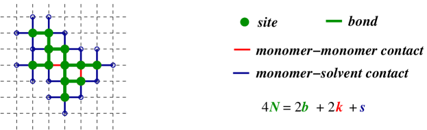
Figure 24: A schematic drawing of an interacting lattice animals which contain a cluster with $b=11$ bonds and $N=12$ sites, and $k=2$ non-bonded monomer-monomer contacts, and $s=22$. It leads to $4N=2b+2k+s$.

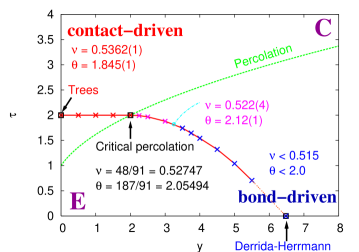
Figure 25: Phase diagram for interacting animals in $d=2$. The full curve separates an extended phase (below) from a collapsed phase (above). At $y=0$ the clusters are trees (minimal number of bonds), while at $\tau=0$ they have no contacts but only bonds. The dashed line corresponds to bond percolation, with the critical point being at $y=\tau=2$. The short dashed-dotted line is a rough estimate for a possible transition between a contact-rich and a bond-rich collapsed phase. The critical exponents $\nu$ and $\theta$ are also shown for different universality classes. Adapted from Ref. Anim2 .

The transition points are determined by the scaling laws of the partition sum:

$$Z_{N}(y,\tau=\tau_{c})\sim\mu(y)^{N}N^{-\theta}$$ (63)

and the gyration radius

$$R_{N}\sim N^{\nu}$$ (64)

where $\mu(y)$ should depend continuously on $y$, but $\theta$ should take discrete values depending on the respective universality. $\nu$ is the Flory exponent. A phase diagram for interacting animals in $d=2$ is shown in Fig. 25. Lattice animals are in the extended phase below the full line, but they are in the collapsed phase above the full line. The bond percolation is described by the dashed curve. The percolation critical point at $y=2$ and $\tau=2$ divides the transition line into two different universality classes. On the left-hand side, the collapse transitions are dominated by non-bonded contacts. In this region PERM simulations are very easy and yield very precise values for the transition curve (which seems to be exactly horizontal) and for the critical exponents. These results have been fully confirmed by field theoretic methods Janssen-anim . For the Derrida-Herrmann model at the far right end of the transition curve, PERM simulations are least efficient, and they could not improve on the results of Derrida . It is not entirely clear whether there exists a further (multi-)critical point between this end point and the percolation point. Such a point, together with an additional phase separation line emanating from it, was suggested by earlier exact enumeration studies (cited in Anim2 ). PERM simulations also weakly suggested such an addition phase separation line, indicated by the short dashed-dotted line in Fig. 25, but these simulations were not easy and interpreting their results was not unambiguous. Indeed, a completely different scenario for the behavior along the transition line between the percolation and Derrida-Herrmann points is suggested in Janssen-anim .

X Protein Folding

In this section we shall only describe applications of a variant of PERM NPERM1 ; NPERM2 to simple lattice models, where it seems one of the most efficient algorithms for finding low energy states. PERM was also applied to continuum models NPERM-AB and was there more efficient than previous Monte Carlo algorithms Stillinger , but has been rendered later obsolete in this application Bachmann-Arkin .

X.1 New Version of PERM (nPERM)

The main improvement of nPERM is that we no longer make identical clones as implemented in old PERM, in order to avoid the loss of diversity which limited the success of old PERM.

When we have a configuration of polymer chains with $n-1$ monomers, we first estimate a predicted weight $W_{n}^{\rm pred}$ for the next step (the $n^{\rm th}$ step), and we count the number $k_{\rm free}$ of free sites where the $n^{\rm th}$ monomer can be placed. If $W_{n}^{\rm pred}>W_{n}^{+}$ and $k_{\rm free}>1$, we make $k$ ($2\leq k\leq k_{\rm free}$) clones with the request that $k$ different sites are chosen for the $n^{\rm th}$ step. Therefore, $k$ configurations with $n$ monomers are forced to be different. If $W_{n}^{\rm pred}<W_{n}^{-}$, a random number $r$ is chosen uniformly in $[0,1]$. If $r<1/2$, the chain is discarded, otherwise it is kept and its weight is doubled. We tried several strategies for selecting $k$ which all gave similar results. Typically, we used $k={\rm min}\left\{k_{\rm free},\left[W_{n}^{\rm pred}/W_{n}^{+}\right]\right\}$.

It is still important to keep the right weight of each configuration with $n$ monomers. When selecting a $k$-tuple $A=\left\{\alpha_{1},\ldots,\alpha_{k}\right\}$ of mutually different continuations $\alpha_{j}$ with probability $p_{A}$, the corresponding weights $W_{n,\alpha 1}$, $\ldots$, $W_{n,\alpha_{k}}$ are

$$W_{n,\alpha_{j}}=\frac{W_{n-1}q_{\alpha_{j}}k_{\rm free}}{k{k_{\rm free}\choose k}p_{A}}\;,\enspace\enspace j=1,2,\ldots,k\;.$$ (65)

Here, the importance

$$q_{\alpha_{j}}=\exp(-\beta E_{n,\alpha_{j}})$$ (66)

of choice $\alpha_{j}$ is the Boltzmann-Gibbs factor associated with the energy $E_{n,\alpha_{j}}$ of the $n^{\rm th}$ placed monomer in the potential created by all previous monomers. The other terms arise from correcting bias and normalization.

Two strategies for the choice of $k$ continuations among $k_{\rm free}$ are described as follows:

1. New PERM with simple sampling (nPERMss):
   $k$ different free sites are chosen randomly and uniformly. The predicted weight is given by,

   $$W_{n}^{\rm pred}=W_{n-1}k_{\rm free}\;,$$ (67)

   and the corresponding weight for each continuation $\alpha_{j}$ is

   $$W_{n,\alpha_{j}}=W_{n-1}q_{\alpha_{j}}k_{\rm free}/k\;$$ (68)

   since there are ${k_{\rm free}\choose k}$ different ways to select a $k$-tuple with equal probability, the probability $p_{A}$ is therefore

   $$p_{A}={k_{\rm free}\choose k}^{-1}\;.$$ (69)

   Here the tuples related by permutations are considered as identical.

2. New PERM with importance sampling (nPERMis):
   $k$ different free sites are chosen according to the modified Boltzmann weight $\tilde{q}_{\alpha_{j}}$ defined by

   $$\tilde{q}_{\alpha_{j}}=(k_{\rm free}^{(\alpha_{j})}+1/2)\exp(-\beta E_{n,\alpha_{j}})$$ (70)

   where $k_{\rm free}^{(\alpha_{j})}$ is the number of free neighbors when the $n^{\rm th}$ monomer is placed at $\alpha_{j}$, and $E_{n,\alpha_{j}}$ is its energy gain. The idea of replacing $q_{\alpha_{j}}$ by $\tilde{q}_{\alpha_{j}}$ is that we anticipate continuations with fewer free neighbors which will contribute less on the long run than continuations with more free neighbors. This is similar to “Markovian anticipation” within the framework of old PERM, described in section Sect. III.2, where the bias for placing a monomer at the next step different from the short-sighted optimal importance sampling was found to be preferable. The predicted weight is now

   $$W_{n}^{\rm pred}=W_{n-1}\sum_{j=1}^{k_{\rm free}}\tilde{q}_{\alpha_{j}}\;.$$ (71)

   Using the requirement that the variance of the weights $W_{n}$ is minimal, the proper choice of the probability $p_{A}$ to select a tuple $A=\left\{\alpha_{i},\ldots,\alpha_{k}\right\}$ is found to be

   $$p_{A}=\frac{\sum_{\alpha_{j}\in A}\tilde{q}_{\alpha_{j}}}{\sum_{A^{\prime}}\sum_{\alpha^{\prime}_{j}\in A^{\prime}}\tilde{q}_{\alpha^{\prime}_{j}}}\;,\enspace\enspace j=1,2,\dots,k_{\rm free}\;.$$ (72)

   If $q_{\alpha_{j}}$ had not been replaced by $\tilde{q}_{\alpha_{j}}$, the variance of $W_{n}$ for fixed $W_{n-1}$ would be zero. For $k=1$, it corresponds to the standard importance sampling, i.e. $p_{A}=p_{\alpha_{j}}=\tilde{q}_{\alpha_{j}}/\sum_{i=1}^{k_{\rm free}}\tilde{q}_{\alpha_{i}}$. The weight at the $n^{\rm th}$ step is thus $W_{n,{\alpha_{j}}}=W_{n-1}q_{\alpha_{j}}/p_{\alpha_{j}}$. For $k>1$, $W_{n,{\alpha_{j}}}$ is given by (65).

A noteworthy feature of both nPERMss and nPERMis is that they cross over to complete enumeration when $W_{n}^{+}$ and $W_{n}^{-}$ tend to zero. In this limit, all possible branches are followed and none is pruned as long as its weight is not strictly zero. In contrast to this, with the use of the original PERM as explained in Sect. II, exponentially many copies of the same configuration would be made. It suggests that one can be more lenient in choosing $W_{n}^{+}$ and $W_{n}^{-}$ when applying nPERM.

X.2 HP Model

For testing the efficiency of the new PERM, we applied it to the HP model Dill since this model is well simulated for bench-marking. In this model, a protein is simplified by replacing amino acids by only two types of monomers, $H$ (hydrophobic) and $P$ (polar) monomers. Therefore a protein (a polymer) of length $n$ is modeled as a self-avoiding chain of $n$ steps on a regular (square or simple cubic) lattice with repulsive or attractive interactions between neighboring non-bonded monomers such that $\epsilon_{HH}=-1$, $\epsilon_{HP}=\epsilon_{PP}=0$. The partition sum is

$$Z_{n}=\sum_{walks}q^{m}$$ (73)

where $q=\exp(-\beta\epsilon_{HH})$ and $m$ is the total number of non-bonded $H-H$ pairs.

In our simulations, we chose the two thresholds $W_{n}-=0$ and $W_{n}^{+}\leq\infty$, i.e. we neither pruned nor branched, for the first configuration hitting length $n$. For the following configurations we used $W_{n}^{+}=C\hat{Z}_{n}/\hat{Z}_{0}(c_{n}/c_{0})^{2}$ and $W_{n}^{-}=0.2\,W_{n}^{+}$. Here, $c_{n}$ is the total number of configurations of length $n$ already created during the run, $\hat{Z}_{n}$ is the partition sum estimated from these configurations, and $C$ is some positive number $\leq 1$. The idea of incorporating the term $(c_{n}/c_{0})^{2}$ is that we can reduce the upper threshold $W_{n}^{+}$ in order to make more cloning in possible branches as a lower energy state is hit but only few configurations of length $n$ have been obtained. The following results were all obtained with $C=1$, though substantial speed-ups (up to a factor 2) could be obtained by choosing $C$ much smaller, typically as small as $10^{-15}$ to $10^{-24}$. The latter is easily understandable: with such small $C$, the algorithm performs essentially exact enumeration for short chains, giving thus maximal diversity, and becomes stochastic only later when following all possible configurations would become unfeasible.

For presenting the efficiency of nPERMss and nPERMis, we applied them to find the ground state of the HP model with blind search. Special comparison is made with the core-directed growth method (CG) of Beutler and Dill bd96 . This is the only method we found to be still competitive with nPERM but it works only for the HP model and relies heavily on heuristics. Two examples are shown here.

(a) Ten sequences of 48-mers in $d=3$ from Ref. yue95 are tested. In Table 1, we list the required CPU time (measured in minutes) per independent ground state hit on a 167 MHz Sun ULTRA I workstation. As with the original PERM Grassberger97 , we could also reach lowest energy states by using nPERM, but the required CPU time is within one order of magnitude shorter than that needed for PERM. For all ten sequences we use the same temperature, $\exp(1/T)=18$, although we could have optimized CPU times by using different temperatures for each chain. Results obtained in Ref. NPERM1 ; NPERM2 are carried out on a SPARC 1 machine which is slower by a factor $\approx 10$ than the Sun workstation. Therefore, in Table 1 we multiplied their results by 10 for comparison. We see that nPERM gave comparable speeds as CG. But, one has to note that the lowest energy of the sequence No.9 was not hit by CG bd96 .

Table 1: Performances for the 3-d binary (HP)- sequences of 48-mers from  yue95 , presented by the CPU time (minutes) per independent ground state hit. The ground state energy is denoted by $E_{\min}$. Results obtained by using PERM PS321998 , nPERMss and nPERMis NPERM1 ; NPERM2 are carried out on a 167 MHz Sun Ultra I workstation. Results quoted from Ref. bd96 obtained by CG are multiplied by 10 for the comparison.

sequence nr.	$-E_{\rm min}$	PERM	nPERMss	nPERMis	CG
1	32	6.9	0.66	0.63	0.94
2	34	40.5	4.79	3.89	3.50
3	34	100.2	3.94	1.99	6.20
4	33	284.0	19.51	13.45	2.90
5	32	74.7	6.88	5.08	1.20
6	32	59.2	9.48	6.60	46.00
7	32	144.7	7.65	5.37	6.40
8	31	26.6	2.92	2.17	3.80
9	34	1420.0	378.64	41.41	-
10	33	18.3	0.89	0.47	0.11

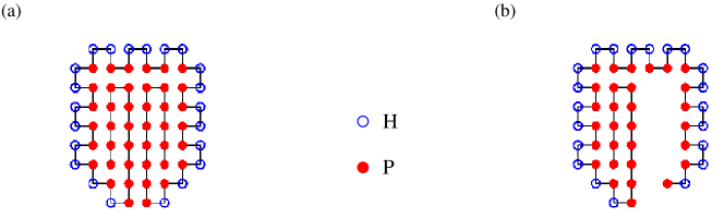
Figure 26: (a) One of the ground state configurations for a $N=64$ chain in 2D from Unger . Other states with the same energy differ in the detailed folding of the tails in the interior, but have identical outer shapes. (b) When about 3/4 of the chain is grown, one has to pass through a very unstable configuration which is stabilized only later, when the hydrophobic core is filled. Adapted from Ref. NPERM1 ; NPERM2

(b) There exists one HP sequence of 64-mers introduced in Ref. Unger , for which it is particularly difficult to find its ground state energy $E_{\rm min}=-42$ by any chain growth algorithm. One of the ground state configuration is shown in Fig. 26(a). Its degeneracies of $E_{\rm min}=-42$ differ in the detailed folding of the tails in the interior. As one uses a chain growth algorithm, it seems very unnatural that the chain has to grow first along an arc (Fig. 26)(b), only until much later that the structure of the chain will be stabilized. It shows the difficulty of folding this HP sequence into its ground state. With nPERM, the ground state was reached with blind search. The average CPU time per ground state hit was about $30$h on the DEC21264, which seems to be roughly comparable to the CPU time needed in Refs. Irback ; PRL831886 , but slower than Ref. bd96 where CG was used. In a previous application of (old) PERM PS321998 , the configuration wirh $E_{\rm min}=-42$ was found only by means of some special tricks (non-blind search) together with the original PERM.

XI DNA Melting

At physiological temperatures, DNA forms the famous double helix. When the temperature is elevated, a point $T_{m}$ is reached where the covalent bonds along the backbone are still strong enough to keep the two strands intact, but the hydrogen bonds between the strands no longer can keep them together. The ensuing separation at temperatures $>T_{m}$ is known as DNA denaturation or DNA melting.

Since the strengths of the hydrogen bonds between pairs A-T and C-G are different, also the melting temperatures $T_{m}$ are different for homogeneous DNA, with $T_{m}(A-T)<T_{m}(C-G)$. For natural DNA, the effective melting temperature depends on the A/C composition, and precise measurements of melting curves for short pieces of DNA can give detailed information about the base composition. This has been used for a long time as one of the easiest and fastest methods to obtain genetic information, and modern developments have made high resolution DNA melting one of the most simple, cheap and fast techniques for genotyping, sequence matching, and mutation scanning Reed .

The sharpness of the transition in case of long homogeneous DNA has suggested since long ago that DNA melting is a first order phase transition Wartell . But the earliest models Poland by Poland and Scheraga could only give rise to a second order transition, which was seen as a severe problem. These models of course lacked many aspects of the real DNA melting problem, such as the helical structure of DNA. This was done in view of the universality of second order phase transitions, and later models that did include the helix structure indeed did not do better.

On the other hand, it was already speculated early on that the excluded volume effect – that was neglected in Poland – could be responsible for the change into a first order transition. The first model that treated the excluded volume effect correctly was published by Coluzzi et al. coluzzi and simulated by means of PERM. The model treated each DNA strand as a SAW on the simple cubic lattice. But the two strands were mutually self avoiding only to the extent that bases that were not supposed to be bound by hydrogen bonds were not allowed to occupy the same lattice site. Base pairs that were bound in the native (non-molten) configuration were not only allowed to occupy the same site, but would also gain an energy $\epsilon$ if they did, mimicking thereby the binding between the two strands. In addition, variants were studied where either the excluded volume effect within each strand and/or between the strands was neglected.

The results were as expected: While all variants that did not incorporate the full excluded volume effect showed second order transitions, the version with full excluded volume interactions showed a first order transition. Later studies, both by simulations (using PERM and other methods) and by analytic arguments confirmed these results (see Richard for references).

XII Summary

In this review we have concentrated on applications of PERM to problems in polymer physics. But PERM can also be applied to other problems where it is important not only to find rare events, but also to estimate the probabilities with which they occur. This includes various reaction-diffusion problems such as the long time tails in the Donsker-Varadhan problem (see Sect. 3) and in the annihilation reaction $A+A\to 0$ Mehra2 , but also to more exotic problems like that of multiple spanning clusters in percolation Grassberger02 . These are all problems where theory makes clear predictions that were very hard to verify numerically with other algorithms. But there are also some other applications of PERM to polymer problems that we have not discussed here, such as polymers grafted to porous Membranes and non-porous Graf-G05 membranes, adsorption of copolymers to surfaces Ads-block , scaling corrections for SAWs on Manhattan lattices Manhattan , and 2-d ISAWs with orientation dependent interactions Barkema .

PERM belongs to a class of Monte Carlo algorithms called sometimes “sequential algorithms with resampling” Liu . In contrast to most other algorithms in this class, it is implemented depth-first which leads to very compact codes and minimal memory requirements. In principle, it can be applied to any problem where instances are built sequentially by repeating small steps. Its main ideas are that these steps can be biased in order to shear the evolution towards the wanted (in general rare but highly weighted) configurations. If this is not deemed successful, the further evolution can be pruned, while very successful trials can be cloned, with each clone evolving further independently. Notice that pruning and cloning are done on partially constructed configurations, with the hope that configurations that are successful at an early stage will also continue to be successful later. When this is true, efficiency can be spectacular (such as for $\Theta$ polymers, Sect. 4). But when it is not true, the method simply fails. Examples of the latter were also discussed in Sects. 3, 4 and 11.

In most applications, the criterion for success is simply the weight of the configuration, based on a combination of Boltzmann, entropic, and bias compensating factors. But in some cases – illustrated in Sect. 9 for lattice animals – the weight itself would be a very poor “fitness” indicator. For lattice animals, a much better fitness function was found empirically.

In addition to the versions of PERM that we have discussed in this review, there exist also “flat” flatPERM and “multicanonical” multiPERM versions of it. Their main advantage is that data over a wide range of energies can be obtained in one single run, while ordinary PERM would need several runs, each covering the energy range that dominates at one particular temperature. This is certainly an attractive feature, but it is not as important as in Markov Chain Monte Carlo algorithms. While it is there highly non-trivial to combine results obtained at different temperatures ferrenberg , this is much easier for PERM where the algorithm provides very precise estimates of the partition sum.

- (1) Flory, P.J.: Principles of polymer chemistry. Cornell University Press, Ithaca, NY (1953)
- (2) Lifshitz, I.M.: JETP 28, 1280- (1968)
- (3) de Gennes, P.G.: Scaling concepts in polymer physics. Cornell University Press, Ithaca, NY (1969)
- (4) Grosberg, A.Yu., Kuznetsov, D.V.: Quantitative theory of the globule-to-coil transition. 1. Link density distribution in a globule and its radius of gyration. Macromolecules 25, 1970-1979 (1992)
- (5) Roiter, Y., Minko, S.: AFM single molecule experiments at the solid-liquid interface: in situ conformation of adsorbed flexible polyelectrolytes chains. J. Am. Chem. Soc. 127, 15688-15689 (2005)
- (6) Salman, H., Zbaida, D. Rabin, Y., Chatenay, D., Elbaum, M.: Kinetics and mechanism of DNA uptake into the cell nucleus. Proc. Natl. Acad. Sci. U. S. A. 98, 7247-7252 (2001)
- (7) Meller, A.: Dynamics of polynucleotide transport through nanometre-scale pores. J. Phys.: Condens. Matter. 15, R581-R607 (2003)
- (8) Kasianowicz, J.J., Brandin, E., Branton, D., Deamer, D.W.: Characterization of individual polynucleotide molecules using a membrane channel. Proc. Nacl. Acad. Sci. U. S. A. 93, 13770-13773 (1996)
- (9) Binder, K. (eds.): Monte Carlo and molecular dynamics simulations in polymer science. Oxford university press, NY (1995)
- (10) Binder, K., Paul, W.: Recent developments in Monte Carlo simulations of lattice models for polymer systems. Macromolecules 41, 4337-4550 (2008)
- (11) Rosenbluth, M.N., Rosenbluth, A.W.: Monte Carlo calculation of the average extension of molecular chains. J. Chem. 23, 356-359 (1955)
- (12) Wall, F.T., Erpenbeck, J.J.: New method for the statistical computation of polymer dimensions. J. Chem. Phys. 30, 634-637 (1959)
- (13) Madras, N., Sokal, A.D.: The pivot algorithm: A highly efficient Monte Carlo method for the self-avoiding walk. J. Stat. Phys. 50, 109-186 (1988)
- (14) Grassberger, P.: Pruned-enriched Rosenbluth method: simulations of polymers of chain length up to . Phys. Rev. E 56, 3682-3693 (1997)
- (15) Anderson, J.B.: A random walk simulation of the Schrödinger equation: H. J. Chem. Phys. 63, 1499-1503 (1975)
- (16) Grassberger, P., Frauenkron, H., Nadler, W.: PERM: a Monte Carlo strategy for simulating polymers and other things, in: Grassberger, P., Barkema, G. Nadler, W. (eds.) Monte Carlo approach to biopolymers and protein folding, pp. 301-315, World Scientific, Singapore (1998)
- (17) Grassberger, P., Nadler, W.: “Go with the winners”-Simulations. In Proceedings of Heraeus Summer School “Vom Billiardtisch bis Monte Carlo: Spielfelder der statistischen Physik”, Chemnitz, October 2000; (cond-mat/0010265)
- (18) Grassberger, P.: Go with the winners: a general Monte Carlo strategy. Computer Physics Communication 147, 64-70 (2002)
- (19) Grassberger P.: Comment on “Polymer localization in attractive random media” [J. Chem. Phys. 109, 1011 (1998)]. J. Chem. Phys. 111, 440 (1999)
- (20) Donsker, M.D., Varadhan, S.R.S: Asymptotics for the Wiener Sausage. Commun. Pure Appl. Math. 28, 525-565 (1975)
- (21) Mehra, V., Grassberger, P.: Transition to localization of biased walks in a randomly absorbing environment. Physica D: Nonlinear phenomena 168-169, 244 (2002)
- (22) Frauenkron, H., Causo, M.S., Grassberger, P.: Two-dimensional self-avoiding walks on a cylinder. Phys. Rev. E 59, R16-R19 (1999)
- (23) Hsu, H.-P., Grassberger, P.: 2-dimensional polymers confined in a strip. Eur. Phys. J. B 36, 209-214 (2003)
- (24) Hsu, H.-P., Grassberger, P.: Polymers confined between two parallel plane walls. J. Chem. Phys. 120, 2034-2041 (2004)
- (25) Duplantier, B.: Geometry of polymer chains near the theta-point and dimensional regularization. J. Chem. Phys. 86, 4233-4244 (1987)
- (26) Hager, J., Schäfer, L.: -point behavior of diluted polymer solutions: Can one observe the universal logarithmic corrections predicted by field theory? Phys. Rev. E 60, 2071–2085 (1999)
- (27) Boothroyd, A.T., Rennie, A.R., Boothroyd, C.B., Fetters, L.J.: Direct measurement of the three-body interaction parameter in a dilute polymer solution. Phys. Rev. Lett. 69, 426-429 (1992)
- (28) Widom, B.: Phase separation in polymer solutions. Physica A 194, 532-541 (1993)
- (29) Frauenkron, H., Grassberger, P.: Critical Unmixing of Polymer Solutions. J. Chem. Phys. 107, 9599-9608 (1997)
- (30) Duplantier, B.: Lagrangian tricritical theory of polymer chain solutions near the -point. J. Physique 43, 991-1020 (1982)
- (31) Grassberger, P., Hsu, H.-P.: Stretched polymers in a poor solvent. Phys. Rev. E 65, 031807 (2002)
- (32) Ferrenberg, A.M., Swendsen, R.H.: New Monte Carlo technique for studying phase transitions. Phys. Rev. Lett. 61, 2635-2639 (1988); Optimized Monte Carlo data analysis. Phys. Rev. Lett. 63, 1195-1198 (1989)
- (33) Prellberg, T., Owczarek, A. L.: Four-dimensional polymer collapse: Pseudo-first-order transition in interacting self-avoiding walks. Phys. Rev. E 62, 3780-3789 (2000); First-order scaling near a second-order phase transition: Tricritical polymer collapse. Europhys. Lett. 51, 602-607 (2000); Four-dimensional polymer collapse II: interacting self-avoiding trails. Physica A 297, 275-290 (2001); Pseudo-first-order transition in interacting self-avoiding walks and trails cond-mat/0108390 (2001)
- (34) Grassberger, P., Christensen, C., Bizhani, G., Son, S.-W., Paczuski, M.: Explosive percolation is continuous, but with unusual finite size behavior. arXiv:1103.3728 (2011)
- (35) Netz, R.R., Andelman, D.: Neutral and charged polymers at interfaces. Phys. Rep. 380, 1-95 (2003)
- (36) Hsu, H.-P., Paul, W., Binder, K.: Polymer chain stiffness versus excluded volume: a Monte Carlo study of the crossover towards the wormlike chain model. Europhys. Lett. 92, 28003 (2010)
- (37) Bastolla U., Grassberger, P.: Phase transitions of single semistiff polymer chains. J. Stat. Phys. 89, 1061-1078 (1997)
- (38) Doniach, S., Garel, T., Orland, H.: Phase diagram of a semiflexible polymer chain in a solvent: application to protein folding. J. Chem. Phys. 105, 1601 (1996)
- (39) Li, B., Madras, N., Sokal, A.D.: Critical exponents, hyperscaling, and universal amplitude ratios for two- and three-dimensional self-avoiding walks. J. Stat. Phys. 80, 661-754 (1995)
- (40) Belohorec, P., Nickel, B.G.: Accurate universal and two-parameter model results from a Monte-Carlo renormalization group study. Guelph University preprint (1997).
- (41) Grassberger, P., Sutter, P., Schäfer, L.: Field theoretic and Monte Carlo analysis of the Domb - Joyce model. J. Phys. A 30, 7039-7056 (1997)
- (42) Domb, C., Joyce, S.,: Cluster expansion for a polymer chain. J. Phys. C 5, 956-976 (1972)
- (43) Hsu, H.-P., Nadler, W., Grassberger, P.: Scaling of star polymers with one to 80 arms. Macromolecules 37, 4658-4663 (2004)
- (44) Grassberger, P. (unpublished).
- (45) Milchev, A., Binder, K.: A polymer chain trapped between two parallel repulsive walls: a Monte-Carlo test of scaling behavior. Eur. Phys. J. B. 3, 477-484 (1988); Eurrtum. Phys. J. B. 13, 607 (2000)
- (46) Eisenriegler, E.: Random walks in polymer physics. In: Meyer-Ortmanns, H., Klümper, A. (eds.) Field Theoretical Tools in polymer and particle physics. Springer, Heidelberg (1997)
- (47) Eisenriegler, E., Kremer, K., Binder, K.: Adsorption of polymer chains at surfaces: Scaling and Monte Carlo analyses. J. Chem. Phys. 77, 6296-6320 (1982)
- (48) Eisenriegler, E.: Universal density-force relations for polymers near a repulsive wall. Phys. Rev. E 55, 3116-3123 (1997)
- (49) Hsu, H.-P., Binder, K., Klushin, L.I., Skvortsov, A.M.: What is the order of the two-dimensional polymer escape transition? Phys. Rev. E 76, 021108 (2007)
- (50) Klushin, L.I., Skvortsov, A.M. Hsu, H.-P., Binder, K.: Dragging a polymer chain into a nanotube and subsequent release. Macromolecules 41, 5890-5898 (2008).
- (51) Hsu, H.-P., Binder, K., Klushin, L.I., Skvortsov, A.M.: Escape transition of a polymer chain from a nanotube: how to avoid spurious results by use of force-biased pruned-enriched Rosenbluth algorithm. Phys. Rev. E 78, 041803 (2008)
- (52) Grassberger, P.: Simulations of grafted polymers in a good solvent. J. Phys. A 38, 323-331 (2005)
- (53) Hsu, H.-P., Grassberger, P.: Effective interactions between star polymers. Europhys Lett. 66, 874-880 (2004)
- (54) Duplantier, B.: Polymer network of fixed topology: renormalization, exact critical exponent in two dimensions, and . Phys. Rev. Lett. 57, 941-944 (1986)
- (55) Barrett, A.J., Tremain, D.L.: Lattice walk models of uniform star polymers with many arms. Macromolecules 20, 1687-1692 (1987)
- (56) Batoulis, J., Kremer, K.: Thermodynamic properties of star polymers: good solvents. Macromolecules 22, 4277-4285 (1989)
- (57) Shida, K., Ohno, K., Kimura, M., Kawazoe, Y.: Monte Carlo study of the second virial coefficient and statistical exponent of star polymers with large numbers of branches. Macromolecules 33, 7655-7662 (2000)
- (58) Di Cecca, A., Freire, J.J.: Monte Carlo simulation of star polymer systems with the bond fluctuation model. Macromolecules 35, 2851-2858 (2002)
- (59) Ohno, K.: Scaling theory and computer simulation of star polymers in good solvents. Condens. Matter Phys. 5, 15-36 (2002)
- (60) Zifferer, G.: Monte Carlo simulation studies of the size and shape of linear and star-branched polymers embedded in the tetrahedral lattice. Macromol. Theory Simul. 8, 433-462 (1999)
- (61) Grest, G.S., Kremer, K., Witten, T.A.: Structure of many-arm star polymers: a molecular dynamics simulation. Macromolecules 20, 1376-1383 (1987)
- (62) Grest, G.S.: Structure of many-arm star polymers in solvents of varying quality: a molecular dynamics study. Macromolecules 27, 3493-3500 (1994)
- (63) Schäfer, L, von Ferber, C, Lehr, U., Duplantier, B.: Renormalization of polymer networks and stars. Nuclear Physics B 374, 473-495 (1992)
- (64) Witten, T.A., Pincus, P.A.: Colloid stabilization by long grafted polymers. Macromolecules 19, 2509 (1986)
- (65) Rubio, A.M., Freire, J.J.: Interaction between two star polymers in a good solvent. Comp. Theory. Polym. Sci., 10, 89-96 (2000)
- (66) Likos, C.N., Löwen, H., Watzlawek, M., Abbas, B., Jucknischke, O., Allgaier, J., Richter, D: Star polymers viewed as ultrasoft colloidal particles. Phys. Rev. Lett. 80, 4450-4453 (1998)
- (67) Hsu, H.-P., Paul, W., Binder, K.: One- and two-component bottle-brush polymers: simulations compared to theoretical predictions. Macromol. Theory & Simul. 16, 660-689 (2007)
- (68) Hsu. H.-P., Paul, W., Binder, K.: Intramolecular phase separation of copolymer “bottle brushes”: No sharp phase transition but a tunable length scale. Europhys. Lett. 76, 526-532 (2006)
- (69) Hsu, H.-P., Paul, W., Binder, K.: Structure of bottle-brush polymers in solutions: a Monte Carlo test of models for the scattering function. J. Chem. Phys. 129, 204904 (2008)
- (70) Hsu, H.-P., Paul, W., Binder, K.: Standard definitions of persistence length do not describe the local “intrinsic” stiffness of real polymer chains. Macromolecules 43, 3094 (2010)
- (71) Daoud, M., Cotton, J. P.: Star shaped polymers : a model for the conformation and its concentration dependence. J. Phys. (Paris) 43, 531 (1982)
- (72) Wang, Z., Safran, S.A.: Size distribution for aggregates of associating polymers. II. Linear packing. J. Chem. Phys. 89, 5323-5328 (1988)
- (73) Ligoure, C., Leibler, L.: Decoration of rough surfaces by chain grafting. Macromolecules 23, 5044-5046 (1990).
- (74) Sevick, E.M.: Shear swelling of polymer brushes grafted onto convex and concave surfaces. Macromolecules 29, 6952-6958 (1996)
- (75) Grest, G.S., Murat, M.: Monte Carlo and molecular dynamics simulations in polymer science, p. 476. In Binder, K.(eds.) Oxford University press, New York (1995)
- (76) Leath, P.L.: Cluster size and boundary distribution near percolation threshold. Phys. Rev. B 14, 5046-5055 (1976)
- (77) Swendsen, R.H., Wang, J.: Nonuniversal critical dynamics in Monte Carlo simulations. Phys. Rev. Lett. 58, 86–88 (1987)
- (78) Hsu, H.-P., Nadler, W., Grassberger, P.: Simulations of lattice animals and trees. J. Phys. A: Math. Gen. 38, 775-806 (2005)
- (79) Janse van Rensburg, E.J., Madras, N.: Metropolis Monte Carlo simulation of lattice animals. J. Phys. A: Math. Gen. 30, 8035-8066 (1997)
- (80) Lubensky, T.C., Isaacson, J.: Field theory for the statistics of branched polymers, gelation, and vulcanization. Phys. Rev. Lett. 41, 829-832 (1978); ERRATA: Field theory for the statistics of branched polymers, gelation, and vulcanization. Phys. Rev. Lett. 42, 410 (1979); Statistics of lattice animals and dilute branched polymers. Phys. Rev. A 20, 2130-2146 (1979)
- (81) Adler, J., Meir, Y., Harris, A.B., Aharony, A.: Series study of random animals in general dimensions. Phys. Rev. B 38, 4941-4954 (1988)
- (82) Jensen, I: Counting polyominoes: a parallel implementation for cluster counting ICCS 2003 ed P M A Sloot et al. Berlin: Springer pp 203–12 (2003)
- (83) You, S, Janse van Rensburg, E.J.: Adsorbing trees in two dimensions: A Monte Carlo study. Phys. Rev. E 64, 046101 (2001)
- (84) Parisi, G., Sourlas, N: Critical behavior of branched polymers and the Lee-Yang edge singularity. Phys. Rev. Lett. 46, 871-874 (1981)
- (85) Janssen, H.K., Lyssy, A.: Adsorption-transition of branched polymers at surfaces: superuniversality of the crossover exponent Europhys. Lett. 29, 25 (1995)
- (86) Miller, J.D., De’Bell, K.: Randomly branched polymers and conformal invariance J. Physique I 3, 1717 (1993)
- (87) Hsu, H.-P., Nadler, W., Grassberger, P.: Violating conformal invariance: two-dimensional clusters grafted to wedges, cones, and branch points of Riemann surfaces. Phys. Rev. E 71, 065104R (4 pages) (2005)
- (88) Lummer, O., Pringsheim, E.: Verhandl. Deutsch. Physikal. Gesellsch. 2, 163 (1900)
- (89) Flesia, S., Gaunt, D.S., Soteros, C.E., Whittington, S.G.: General model for collapse in lattice animals. J. Phys. A: Math. Gen. 25, L1169 (1992)
- (90) Hsu, H.-P., Grassberger, P.: Collapsing lattice animals and lattice trees in two dimensions. J. Stat. Mech., p06003 (2005)
- (91) Derrida, B., Herrmann, H.J.: Collapse of branched polymers. J. Physique 44, 1365-1376 (1983)
- (92) Janssen, H.-K., Stenull, O.: The collapse transition of randomly branched polymers -renormalized field theory. arXiv:1102.3439 (2011)
- (93) Hsu, H.-P., Mehra, V., Nadler, W., Grassberger, P.: Growth algorithms for lattice heteropolymers at low temperatures. J. Chem. Phys. 118, 444-451 (2003)
- (94) Hsu, H.-P., Mehra, V., Nadler, W., Grassberger, P.: Growth-based optimization algorithm for lattice heteropolymers. Phys. Rev. E 68, 021113 (2003)
- (95) Hsu, H.-P., Mehra V., Grassberger, P.: Structure optimization in an off-lattice protein model. Phys. Rev. E 68, 037703 (2003)
- (96) Stillinger, F.H., Head-Gordon, T., Hirshfeld, C.L.: Toy model for protein folding. Phys. Rev. E 48, 1469-1477 (1993); Stillinger F.H., Head-Gordon, T.: Collective aspects of protein folding illustrated by a toy model. Phys. Rev. E 52, 2872-2877 (1995)
- (97) Bachmann, M., Arkin, H., Janke, W.: Multicanonical study of coarse-grained off-lattice models for folding heteropolymers. Phys. Rev. E 71, 031906 (2005)
- (98) Dill, K. A.: Theory for the folding and stability of globular proteins Biochemistry 24, 1501-1509 (1985).
- (99) Beutler, T.C., Dill, K.A.: A fast conformational search strategy for finding low energy structures of model proteins. Protein Sci. 5, 2037-2043 (1996)
- (100) Yue, K., Fiebig, K.M., Thomas, P.D., Chan, H.S., Shakhnovich, E.I., Dill, K.A.: A test of lattice protein folding algorithms. Proc. Natl. Acad. Sci. USA 92, 325 (1995).
- (101) Unger, R., Moult, J: Genetic algorithms for protein folding simulations. J. Mol. Biol. 231, 75-81 (1993)
- (102) Bastolla, U., Frauenkron, H., Gerstner, E., Grassberger, P., Nadler, W.: Testing a new Monte Carlo algorithm for protein folding. Proteins 32, 52-66 (1998)
- (103) Irbäck, A. in Monte Carlo Approach to Biopolymers and Protein Folding, edited by Grassberger, P. et al. (World Scientific, Singapore, 1998), pp. 98-109.
- (104) Chikenji, G., Kikuchi, M., Iba, Y.: Multi-self-overlap ensemble for protein folding: ground state search and thermodynamics. Phys. Rev. Lett. 83, 1886-1889 (1999); Chikenju, G. Kikuchi, M.: What is the role of non-native intermediates of -lactoglobulin in protein folding? Proc. Natl. Acad. Sci. U.S.A. 97, 14273-14277 (2000)
- (105) Wartell, R.M., Benight, A.S.: Thermal denaturation of DNA molecules: A comparison of theory with experiment Phys. Rep. 126, 67-107 (1985)
- (106) Reed, G.H., Kent, J.O., Wittwer, C.T.: High-resolution DNA melting analysis for simple and efficient molecular diagnostics. Pharmacogenomics 8, 597-608 (2007)
- (107) Poland, D., Scheraga, H.A.: Phase transitions in one dimension and the helix-coil transition in polyamino acids J. Chem. Phys. 45, 1456-1463 (1966); Occurrence of a phase transition in nucleic acid models J. Chem. Phys. 45, 1464-69 (1966)
- (108) Causo, M.S., Coluzzi, B., Grassberger, P.: Simple model for the DNA denaturation transition. Phys. Rev. E 62, 3958-3973 (2000)
- (109) Richard, C., Guttmann, A.J.: Poland-Scheraga Models and the DNA Denaturation Transition J. Stat. Phys. 115, 925-947 (2003)
- (110) Mehra, V., Grassberger, P.: Trapping reaction with mobile traps. Phys. Rev. E 65, 050101(R) (2002)
- (111) Hsu, H.-P., Grassberger, P.: Polymers grafted to porous membranes. Europhys Lett. 77, 18003 (4 pages) (2007)
- (112) Bhattacharya, S., Hsu, H.-P., Milchev, A., Rostiashvili, V. G., Vilgis, T. A.: Adsorption of multi-block and random copolymers on a solid surface: critical behavior and phase diagram. Macromolecules 41, 2920-2030 (2008)
- (113) Caracciolo, S., Causo, M.S., Grassberger, P,, Pelissetto, A.: Determination of the exponent for SAWs on the two-dimensional Manhattan lattice J. Phys. A: Math. Gen. 32, 2931-2948 (1999)
- (114) Barkema, G.T., Bastolla, U., Grassberger, P.: Two-dimensional oriented self-avoiding walks with parallel contacts J. Stat. Phys. 90, 1311-1324 (1998)
- (115) Liu, J.S.: Monte Carlo strategies in scientific computing. Springer, New York (2008)
- (116) Prellberg, T., Krawczyk, J.: Flat histogram version of the pruned and enriched Rosenbluth method. Phys. Rev. Lett. 92, 120602 (2004)
- (117) Bachmann, M., Janke, W.: Multicanonical Chain-Growth Algorithm. Phys. Rev. Lett. 91, 208105 (2003)