Isocurvature modes and Baryon Acoustic Oscillations II: gains from combining CMB and Large Scale Structure

Abstract:

We consider cosmological parameters estimation in the presence of a non-zero isocurvature contribution in the primordial perturbations. A previous analysis showed that even a tiny amount of isocurvature perturbation, if not accounted for, could affect standard rulers calibration from Cosmic Microwave Background observations such as those provided by the Planck mission, affect Baryon Acoustic Oscillations interpretation, and introduce biases in the recovered dark energy properties that are larger than forecasted statistical errors from future surveys.

Extending on this work, here we adopt a general fiducial cosmology which includes a varying dark energy equation of state parameter and curvature. Beside Baryon Acoustic Oscillations measurements, we include the information from the shape of the galaxy power spectrum and consider a joint analysis of a Planck-like Cosmic Microwave Background probe and a future, space-based, Large Scale Structure probe not too dissimilar from recently proposed surveys.

We find that this allows one to break the degeneracies that affect the Cosmic Microwave Background and Baryon Acoustic Oscillations combination. As a result, most of the cosmological parameter systematic biases arising from an incorrect assumption on the isocurvature fraction parameter $f_{iso}$, become negligible with respect to the statistical errors. We find that the Cosmic Microwave Background and Large Scale Structure combination gives a statistical error $\sigma(f_{iso})\sim 0.008$, even when curvature and a varying dark energy equation of state are included, which is smaller than the error obtained from Cosmic Microwave Background alone when flatness and cosmological constant are assumed. These results confirm the synergy and complementarity between Cosmic Microwave Background and Large Scale Structure, and the great potential of future and planned galaxy surveys.

1 Introduction

The standard cosmological model assumes adiabatic initial conditions for the perturbations. This simple adiabatic picture is well-motivated as it is predicted by the simplest inflationary single-field models [1, 2], and so far it provides an excellent fit to current data (e.g., [3]). There is however no a priori reason to discard more general initial conditions involving entropy isocurvature perturbations as they can arise from several different mechanisms e.g., multi-field inflation, [4, 5, 6, 7, 8, 9, 10], neutrino isocurvature perturbations [11], axion dark matter [12, 13, 14, 15, 16, 17, 18, 19, 20] or the curvaton scenario [21, 22, 23]. Pure isocurvature models have been observationally excluded [24, 25, 26, 27], but current observations still allow for an admixture of adiabatic and isocurvature contributions [3, 28, 29, 30, 31, 32].

To date, Cosmic Microwave Background (CMB) data have been the main source of information not just about cosmological parameters but also about the nature of cosmological initial conditions. Relaxing the assumption of adiabaticity and allowing an isocurvature contribution introduces new degeneracies in the parameters space which weaken considerably cosmological constraints e.g., [34, 30, 40, 35, 33, 36, 37]. Up to now, the CMB temperature power spectrum alone has not been able to break the degeneracy between the nature of initial perturbations (i.e. the amount and properties of an isocurvature component) and cosmological parameters; adding external data sets somewhat alleviates this issue for some degeneracy directions e.g., [28, 31]. As shown in [38], the precision polarization measurements of future and on-going CMB experiments like Planck will be crucial to lift such degeneracies.

Ref. [39] investigated the effect of relaxing the hypothesis of purely adiabatic initial conditions and found that even a tiny isocurvature fraction contribution, if not accounted for, can lead to an incorrect determination of the cosmological parameters and can affect the standard ruler calibration from the CMB. In fact, the presence of an isocurvature component changes the shape and the location of the CMB acoustic peaks, mimicking the effect of parameters such as $\Omega_{m_{0}}h^{2}$, $H_{0}$ and $w$ (see also [30] and references therein). Ref. [39] found that this has a crucial effect on “standard rulers”, like the sound horizon at radiation drag, inferred from CMB observations. This is of relevance for the next generation of galaxy surveys which aims at probing with high accuracy the late time expansion and thus the nature of dark energy by means of Baryon Acoustic Oscillations (BAO) at low redshift ($z<2$). In fact, for Large Scale Structure (LSS), even a tiny isocurvature fraction contribution, if not accounted for, can affect the BAO estimation, introducing systematics in the BAO observables which can be larger than the statistical errors expected from future surveys.

BAO measurements from galaxy surveys have the potential to be an unprecedented powerful probe of the low redshift Universe, and thus of dark energy ([55, 54, 56] and references therein). The BAO in the primordial photon-baryon fluid, responsible for the characteristic peak structure of the CMB power spectrum, leave, in fact, an imprint in the large scale matter distribution and, at each redshift, their physical properties are related to the size of the sound horizon $r_{s}(z_{d})$ at radiation drag (i.e., when baryons were released from the photons). Since the CMB in principle can precisely provide the standard ruler, i.e. $r_{s}(z_{d})$, by measuring the BAO location at low redshift with LSS surveys, it is possible to probe the expansion history, i.e., the Hubble parameter $H(z)$, and the angular diameter distance $D_{A}(z)$ at different redshifts, and thus the dark energy properties.

It has been found that the effect of a number of theoretical systematics such as non-linearities, bias etc., on the determination of the BAO location can be minimized to the point that BAO are one of the key observables of the next generation dark energy experiments. However, it is important to investigate and test the robustness of the method to all possible theoretical uncertainties.

The analysis in Ref. [39] focused on the forecasts from a CMB-only Planck-like experiment to quantify the impact of the isocurvature contribution on cosmological parameter estimation and degeneracies with $r_{s}(z_{d})$ and, therefore, with BAO measurements. Here we extend the work to a joint analysis of a CMB Planck-like experiment combined to a future space-based LSS survey with characteristics not too dissimilar from the proposed Euclid mission. One of the key points is to see whether adding the full cosmological information provided by future LSS surveys could eventually break the degeneracies introduced by the presence of an isocurvature fraction in the initial conditions. In the present work in fact, we exploit, in the LSS case, not only the information enclosed in the BAO positions, but include the galaxy power spectrum shape adopting the so-called “$P(k)$-method marginalised over growth information” [41, 65]. Moreover we consider spatial curvature and a more general case of dark energy with a varying equation of state parametrized by $w_{0}$ and $w_{a}$.

The rest of the paper is organized as follows. In Sec. 2 we review theory and notation for isocurvature perturbations. In Sec. 3 we outline our methodology, paying particular attention to the method used to compute expected constraints from LSS surveys, including not only the BAO location measurements but also the power spectrum shape. We present our results in Sec. 4 and the conclusions in Sec. 5.

2 Isocurvature: theory and notation

Even if pure isocurvature models have been ruled out [24, 25, 26, 27], current observations allow for mixed adiabatic and isocurvature contributions [3, 28, 29, 30, 31, 32].

In fact, besides primordial adiabatic perturbations, there can exist the so-called isocurvature or entropy perturbations. These are associated to fluctuations in number density between different components of the cosmological plasma in the early Universe, well before photon decoupling, and are generated by stress fluctuations through the causal redistribution of matter under energy-momentum conservation.

Density perturbations are then produced by non-adiabatic pressure (entropy) perturbations (see [42] for a detailed description).

The entropy perturbation between two particle species (i.e., fluid components) can be written in terms of the density contrast $\delta_{i}=\delta\rho_{i}/\rho_{i}$ and the equation of state parameter $w_{i}$ as :

$${\cal S}_{XY}=\frac{\delta_{X}}{1+w_{X}}-\frac{\delta_{Y}}{1+w_{Y}},$$ (1)

which quantifies the variation in the particle number densities between two different species, and it is equivalent to ${\cal S}_{XY}=\delta n_{X}/n_{X}-\delta n_{Y}/n_{Y}$.

The most general description of a primordial perturbation accounts for 5 non-decaying (regular) modes corresponding to each wavenumber: an adiabatic (AD) growing mode, a baryon isocurvature mode (BI), a cold dark matter isocurvature mode (CDI), a neutrino density mode (NID) and a neutrino velocity mode (NIV) (see [11] and references therein). For the dark matter component $\delta n_{c}/n_{c}=\delta\rho_{c}/\rho_{c}$, so that the CDM isocurvature mode can be written as:

$${\cal S}_{c}\equiv\delta_{c}-\frac{3}{4}\delta_{\gamma},$$ (2)

where $\delta_{X}=\delta\rho_{X}/\rho_{X}$ is the energy density contrast of the X particle species. The baryon (b) and the neutrino ($\nu$) isocurvature modes take the form:

$${\cal S}_{b}\equiv\delta_{b}-\frac{3}{4}\delta_{\gamma}$$ (3)

$${\cal S}_{\nu}\equiv\frac{3}{4}\delta_{\nu}-\frac{3}{4}\delta_{\gamma}.$$ (4)

For the adiabatic mode $S_{c}=S_{\nu}=S_{b}=0$.

One of the crucial distinctions between the adiabatic and the isocurvature models relies on the behavior of the fluctuations at very early time, during horizon crossing at the epoch of inflation (or an analogous model for the very early Universe). In the adiabatic case, constant density perturbations are present initially and imply a constant curvature on super-horizon scales, while in the pure isocurvature case there are not initial density fluctuations which, instead, are created from stresses in the radiation-matter component.

An example of isocurvature model is represented by the curvaton scenario [21, 22, 23], which is an alternative to the single field inflationary model. This model relies on the inflaton, the light scalar field that dominates the background density during inflation, and the curvaton field $\sigma$ which, decaying after inflation, seeds the observable cosmological perturbations. The initial conditions then correspond to purely entropy primordial fluctuations, namely isocurvature perturbations, because the curvaton field practically does not contribute to metric perturbations. Besides the fact that current data are compatible with this theoretical picture, the curvaton model attracted growing attention because it predicts primordial non-gaussianity features of the local type in the spectrum of primordial perturbations.

2.1 Notation

A common parametrization for the isocurvature perturbations is given by [43]:

$$f_{iso}=\frac{\langle{\cal{S}}^{2}_{rad}\rangle^{1/2}}{\langle{\cal{R}}^{2}_{rad}\rangle^{1/2}},$$ (5)

defined as the ratio between the entropy ${\cal{S}}$ and the curvature (adiabatic) ${\cal{R}}$ perturbations evaluated during the radiation epoch and at a pivot scale $k_{0}$. In our case we set $0.002\;{\rm Mpc^{-1}}$, as often done in the literature [44, 3]. The correlation coefficient can be then defined in terms of an angle, $\Delta_{k_{0}}$, such that:

$$\cos\Delta_{k_{0}}=\frac{\langle{\cal{R}}_{rad}{\cal{S}}_{rad}\rangle}{\langle{\cal{R}}^{2}_{rad}\rangle^{1/2}\langle{\cal{S}}^{2}_{rad}\rangle^{1/2}}.$$ (6)

Throughout this paper we will use a sign convention such that $f_{iso}<0$ will correspond to correlated modes.

2.2 Isocurvature and CMB

In general the two-point correlation function or power spectra for the adiabatic mode, the isocurvature mode and their cross-correlation can be described by two amplitudes, one correlation angle and three independent spectral indices ($n_{ad}$, $n_{iso}$, $n_{cor}$), so that, in the case of the CMB, the respective algular power spectra are:

$$C_{\ell}^{ad}=\int\frac{dk}{k}[\Theta^{ad}_{\ell}(k)]^{2}\left(\frac{k}{k_{0}}\right)^{n_{ad}-1},$$ (7)

$$C_{\ell}^{iso}=\int\frac{dk}{k}[\Theta^{iso}_{\ell}(k)]^{2}\left(\frac{k}{k_{0}}\right)^{n_{iso}-1}$$ (8)

and

$$C_{\ell}^{cor}=\int\frac{dk}{k}\Theta^{ad}_{\ell}(k)\Theta^{iso}_{\ell}(k)\left(\frac{k}{k_{0}}\right)^{n_{cor}+\frac{1}{2}(n_{ad}+n_{iso})-1}.$$ (9)

Here $\Theta^{ad}_{\ell}(k)$ and $\Theta^{iso}_{\ell}(k)$ are the radiation transfer functions for adiabatic and isocurvature perturbations that describe how an initial perturbation evolved to a temperature or polarization anisotropy multipole $\ell$. The total angular power spectrum takes then the form:

$$C_{\ell}=\langle{\cal{R}}^{2}_{rad}\rangle[C_{\ell}^{ad}+f^{2}_{iso}C_{\ell}^{iso}+2f_{iso}\cos\Delta_{k_{0}}C_{\ell}^{cor}].$$ (10)

From Eq. (10) it is clear that, for small isocurvature fractions, the main isocurvature contribution come from the mixing term coefficient ($2f_{iso}\cos\Delta_{k_{0}})$.

2.3 Isocurvature and LSS

The power spectra of both adiabatic and isocurvature perturbations, as well as their cross-correlation, can be parametrized by three power laws with three amplitudes and three spectral indices $n_{ad}$, $n_{iso}$ and $n_{cor}$:

$$\Delta_{{\cal R}}^{2}(k) \equiv \frac{k^{3}}{2\pi^{2}}\langle{\cal R}_{{\rm rad}}^{2}\rangle=\frac{k_{0}^{3}}{2\pi^{2}}A^{2}\left(\frac{k}{k_{0}}\right)^{n_{ad}-1}\,,$$ (11)

$$\Delta_{{\cal S}}^{2}(k)\! \equiv \!\frac{k^{3}}{2\pi^{2}}\langle{\cal S}_{\rm{rad}}^{2}\rangle=\frac{k_{0}^{3}}{2\pi^{2}}B^{2}\left(\frac{k}{k_{0}}\right)^{n_{iso}-1}\,,$$

$$\Delta_{{\cal R}{\cal S}}^{2}(k)\! \equiv \!\frac{k^{3}}{2\pi^{2}}\langle{\cal R}_{\rm rad}{\cal S}_{\rm rad}\rangle\,$$

$$= \frac{k_{0}^{3}}{2\pi^{2}}A\,B\,\cos\Delta_{k_{0}}\left(\frac{k}{k_{0}}\right)^{n_{cor}+{1\over 2}(n_{ad}+n_{iso})-1}\,.$$

As before, ${\cal R}_{\rm rad}$ stands for the curvature perturbation, and ${\cal S}_{\rm rad}=(\delta_{\rm c}-3\delta_{\gamma}/4)_{\rm rad}$ for the CDI perturbation evaluated during the radiation epoch at a pivot scale $k_{0}$ such that: $A=\langle{\cal R}_{\rm rad}^{2}\rangle^{1/2}$ and $B=\langle{\cal S}_{\rm rad}^{2}\rangle^{1/2}$.

The last of Eqs. (11) refers to the extra-correlation that can be generated by the partial conversion of isocurvature into adiabatic perturbations after the end of inflation.

Since we are interested in the effect of a model with a mixed adiabatic+isocurvature CDI contribution to the LSS, it is useful to give the explicit formula of the shape of the linear matter power spectrum (e.g. [29]):

$$P(k)=(A^{2}+B^{2})[(1-\alpha)\,P^{\rm ad}(k)+\alpha\,P^{\rm iso}(k)+2\beta\sqrt{\alpha(1-\alpha)}\,P^{\rm cor}(k)]\,.$$ (12)

Here $P^{\rm ad}$ and $P^{\rm iso}$ are computed from the initial conditions $({\cal R}_{\rm rad}(k),{\cal S}_{\rm rad}(k))=((1,0)$, $(0,1))$, and:

$$\alpha=\frac{f^{2}_{iso}}{(1+f^{2}_{iso})},\;\beta=\cos(\Delta_{k_{0}}),$$ (13)

where maximally correlated (anticorrelated) modes correspond to $\beta=+1$ ( $\beta=-1$).

The extra cross-correlated term is given by

$$P^{\rm cor}(k)=-(k/k_{0})^{n_{cor}}[P^{\rm ad}(k)P^{\rm iso}(k)]^{{1\over 2}}.$$ (14)

In this paper we adopt the curvaton scenario as a working example for a model that gives rise to a small fraction of correlated CDI isocurvature. As shown in the next sections, our analysis can be generalized to models with an arbitrary amount and type of isocurvature. In general, by tuning the decay dynamics of $\sigma$, the curvaton scenario allows for mixed adiabatic and isocurvature fluctuations, with any residual isocurvature perturbation correlated or anti-correlated to the adiabatic density one, and with the same tilt for both spectra. Our findings are therefore quantitative only for this case, however our conclusions will not be too dissimilar for a model such as the axion-like isocurvature, where $n_{iso}$ is fixed to be 1, given that $n_{ad}$ is not too far away from scale invariance.

In our model we assume $\beta=-1$, $n_{s}\equiv n_{ad}=n_{iso}$ and $n_{cor}=0$.

3 Method

In order to extend the analysis done in Ref. [39] on the impact of an isocurvature contribution on cosmological parameter estimation, we compute joint Fisher matrix forecasts [46] for a CMB Planck-like experiment combined with a future space-based LSS survey with characteristics not too dissimilar from those of the proposed Euclid mission. In what follow we will refer to such a survey as “Euclid-like” or “LSS survey” and use the specifications reported in [47]. We adopt the empirical redshift distribution of H$\alpha$ emission line galaxies derived by [69] from observed H$\alpha$ luminosity functions, and the bias function derived by [70] using a galaxy formation simulation. In particular, we choose a flux limit of 3$\times 10^{-16}$erg s^-1cm^-1, a survey area of 20,000 deg², a redshift success rate $e=0.35$, a redshift accuracy of $\sigma_{z}/(1+z)\leq 0.001$, and a redshift range $0.45\leq z\leq 2.05$. See Tab. 1 for a summary of the experimental specifications.

In both cases we assume a curvaton fiducial model with mixed adiabatic and isocurvature initial conditions. The fiducial value chosen for the isocurvature parameter is $f_{iso}=-0.08$. This is well within the WMAP7-only and slightly outside the WMAP7+BAO+SN 95%CL limits [3, 45]. On the other hand, these bounds are obtained assuming a $\Lambda$CDM model, while accounting for curvature and a varying dark energy equation of state weakens considerably the constraints on the isocurvature contribution [30, 31].

In any case it is important to stress that the Fisher analysis results, as found also by Ref. [39], are not strongly affected by the choice of the fiducial values of the isocurvature amount within these limits.

The set of parameters we use is:

$${\bf q_{\alpha}}=\{\Omega_{m_{0}},\Omega_{X_{0}},\Omega_{b_{0}},h,n_{s},w_{0},w_{a},\log(10^{10}A_{\rm tot}),f_{iso}\}$$ (15)

with fiducial values:

$${\bf\hat{q}_{\alpha}}=\{0.2707,0.7293,0.0451,0.703,0.966,-0.95,0,1.3909,-0.08\},$$ (16)

where $\Omega_{m_{0}}$, $\Omega_{X_{0}}$ and $\Omega_{b_{0}}$ are, respectively, the total matter, dark energy and baryon density parameters at present time, $h$ is related to the Hubble parameter by $H_{0}=100\,h$ Km/(sec Mpc), $n_{s}$ and $A_{\rm tot}$ are the scalar spectral index and the total amplitude accounting for both the adiabatic and the isocurvature contributions, $w_{0}$ and $w_{a}$ are related to the dark energy equation of state parameter $w(z)$ via the standard CPL parametrization [49, 50]:

$$w(z)=w_{0}+w_{a}\frac{z}{1+z}.$$ (17)

Finally, $f_{iso}$ is the isocurvature fraction parameter of Eq. (5) (see §2 for detals). We assume flatness in the fiducial model but $\Omega_{m_{0}}$ and $\Omega_{X_{0}}$ are free parameters in the Fisher matrix computation: the curvature $\Omega_{k}=1-\Omega_{m_{0}}-\Omega_{X_{0}}$ is not fixed and it is a parameter in the analysis.

Recall that, in the case of a CMB-only Planck-like experiment, the constraints on the isocurvature contribution are considerably weakened when $\Omega_{k}$ is a free parameter, and, when also a varying dark energy equation of state is considered, the cosmological constraints from CMB alone weaken even more because of degeneracies [31].

As previously mentioned, in Ref. [39] it was shown that even a small isocurvature contribution, if not accounted for, can lead to an incorrect determination of the cosmological parameters and can affect the $r_{s}(z_{d})$ calibration from the CMB; this affects the BAO location estimation and, therefore, leads to systematic shifts in the derived cosmological parameters, shifts that result to be larger than statistical errors from forthcoming LSS surveys. One of the main purpose of this work is to see if this is still the case for a joint analysis of CMB and LSS when the information from the $P(k)$-shape are included. Therefore, here we extend the work of Ref. [39] not only by including curvature and dark energy parameters in the analysis, but also by exploiting BAO location measurements combined to the galaxy power spectrum shape. The additional cosmological information in the power spectrum should help break degeneracies and thus indirectly improve constraints on the isocurvature parameter.

3.1 Fisher matrix approach

We combine the cosmological information of a CMB experiment like Planck (enclosed in the $F^{CMB-Planck}$ Fisher matrix) and a galaxy survey like Euclid (enclosed in the $F^{LSS}$ Fisher matrix), so our full Fisher matrix is:

$$F_{ij}\equiv F^{CMB-Planck}_{ij}+F^{LSS}_{ij}.$$ (18)

The Fisher matrix is defined as the second derivative of the natural logarithm of the likelihood surface about the maximum. In the approximation that the posterior distribution for the parameters is a multivariate Gaussian with mean $\mbox{\boldmath${\mu}$}\equiv\langle{\bf x}\rangle$ and covariance matrix ${\bf C}\equiv\langle{\bf x}{\bf x}^{t}\rangle-\mbox{\boldmath${\mu}$}\mbox{\boldmath${\mu}$}^{t}$, its elements are given by [51, 52, 53, 46]

$$F_{ij}=\frac{1}{2}{\rm Tr}\left[{\bf C}^{-1}{\partial{\bf C}\over\partial\theta_{i}}{\bf C}^{-1}{\partial{\bf C}\over\partial\theta_{j}}\right]+{\partial\mbox{\boldmath${\mu}$}\over\partial\theta_{i}}^{t}{\bf C}^{-1}{\partial\mbox{\boldmath${\mu}$}\over\partial\theta_{j}},$$ (19)

where ${\bf x}$ is a N-dimensional vector representing the data set, whose components $x_{i}$ are, for example, the fluctuations in the galaxy density relative to the mean in $N$ disjoint cells that cover the three-dimensional survey volume in a fine grid. The $\{\theta_{i}\}$ denote the cosmological parameters within the assumed fiducial cosmology.

For the CMB Fisher matrix set up see appendix A and Tab. 1, for the LSS Fisher matrix set up we follow closely Ref. [41] as follows.

Channels (in GHz)	100	143	217
Beam FWHM	9.5	7.1	5
Temperature sensitivity $\sigma_{T}$ ($\frac{\mu K}{K}$)	2.5	2.2	4.8
Polarization sensitivity $\sigma_{P}$ ($\frac{\mu K}{K}$)	4	4.2	9.8
$z_{min}$	$z_{max}$	Survey Area (deg2)	$\Delta z_{bin}$
0.45	2.05	20.000	0.1

Table 1: TOP: experimental specifications for the Planck experiment. BOTTOM: LSS survey settings, i.e. redshift range $z_{min}$ and $z_{max}$, survey area (A) in squared degrees, and width of the redshift bin $\Delta z_{bin}$.

3.2 Large scale structure treatment

In order to explore the cosmological parameter constraints from a given redshift survey, we need to specify the measurement uncertainties of the galaxy power spectrum. The statistical error on the measurement of the galaxy power spectrum $P_{\rm g}(k)$ at a given wave-number bin is [48]

$$\left[\frac{\Delta P_{\rm g}}{P_{\rm g}}\right]^{2}=\frac{2(2\pi)^{2}}{V_{\rm survey}k^{2}\Delta k\Delta\mu}\left[1+\frac{1}{n_{\rm g}P_{\rm g}}\right]^{2},$$ (20)

where $n_{\rm g}$ is the mean number density of galaxies, $V_{\rm survey}$ is the comoving survey volume of the galaxy survey, and $\mu$ is the cosine of the angle between $\bf{k}$ and the line-of-sight direction $\mu=\vec{k}\cdot\hat{r}/k$.

In general, the observed galaxy power spectrum is different from the true spectrum, and it can be reconstructed approximately assuming a reference cosmology (which we consider to be our fiducial cosmology) as (e.g. [54])

$$P_{\rm obs}(k_{{\rm ref}\perp},k_{{\rm ref}\parallel},z)=\frac{D\!_{A}(z)_{\rm ref}^{2}H(z)}{D\!_{A}(z)^{2}H(z)_{\rm ref}}P_{\rm g}(k_{{\rm ref}\perp},k_{{\rm ref}\parallel},z)+P_{\rm shot}\,,$$ (21)

where

$$P_{\rm g}(k_{{\rm ref}\perp},k_{{\rm ref}\parallel},z)=b(z)^{2}\left[1+\beta(z)\frac{k_{{\rm ref}\parallel}^{2}}{k_{{\rm ref}\perp}^{2}+k_{{\rm ref}\parallel}^{2}}\right]^{2}\times P_{{\rm matter}}(k,z)\,.$$ (22)

In Eq. (21), $H(z)$ and $D_{A}(z)$ are the Hubble parameter and the angular diameter distance, respectively, and the prefactor $(D\!_{A}(z)_{\rm ref}^{2}H(z))/(D\!_{A}(z)^{2}H(z)_{\rm ref})$ encapsulates the geometrical distortions due to a reference cosmology different from the true one [54, 57]. The quantities evaluated in the reference cosmology are distinguished by the subscript ‘ref’, while those in the true cosmology have no subscript. $k_{\perp}$ and $k_{\parallel}$ are the wave-numbers across and along the line of sight in the true cosmology, and they are related to the wave-numbers calculated assuming the reference cosmology by $k_{{\rm ref}\perp}=k_{\perp}D_{A}(z)/D_{A}(z)_{\rm ref}$ and $k_{{\rm ref}\parallel}=k_{\parallel}H(z)_{\rm ref}/H(z)$. $P_{shot}$ is the unknown shot noise that remains even after the conventional shot noise of inverse number density has been subtracted and which we assume to be white noise [54]. Such contribution could arise from galaxy clustering bias even on large scales due to local bias [58] or to misestimates of the local density. In Eq. (22), $b(z)$ is the linear bias factor between galaxy and matter density distributions, and $\beta(z)=f_{g}(z)/b(z)$ is the linear redshift-space distortion parameter [59]. Thus our analysis is limited to large enough scales where bias is scale-independent (we will return to this below). We estimate $f_{g}(z)$ by integration of the evolution equations of the linear density perturbations. The linear matter power spectrum $P_{{\rm matter}}(k,z)$ in Eq. (21) takes the form

$$P_{{\rm matter}}(k,z)=\frac{8\pi^{2}c^{4}k_{0}A_{\rm tot}}{25H_{0}^{4}\Omega_{m}^{2}}T^{2}(k)\left[\frac{G(z)}{G(z=0)}\right]^{2}\left(\frac{k}{k_{0}}\right)^{n_{s}}e^{-k^{2}\mu^{2}\sigma_{r}^{2}},$$ (23)

where $G(z)$ is the linear growth-factor, whose fiducial value in each redshift bin is computed through numerical integration of the differential equations governing the growth of linear perturbations in the presence of dark energy [60]. The linear transfer function $T(k)$ depends on matter and baryon densities (neglecting dark energy at early times), and is computed in each redshift bin using CAMB [61] modified to include the isocurvature contribution. The parameter $A_{\rm tot}$ refers to the amplitude accounting for both the adiabatic and the isocurvature contributions as described in §2.3, and $n_{s}$ is the spectral index which in our case reads $n_{s}\equiv n_{ad}=n_{iso}$, so that it can be factorized out in the $P_{{\rm matter}}(k,z)$ expression in Eq. (23).

Moreover, in Eq. (23) we have added the damping factor exp($-k^{2}\mu^{2}\sigma_{r}^{2}$), due to redshift uncertainties, where $\sigma_{r}=(\partial r/\partial z)\sigma_{z}$, $r(z)$ being the comoving distance [62, 54].

From the above, it should be clear that, when adding LSS, we exploit the information from both the galaxy power spectrum shape and BAO distance indicators.

In each redshift shell, with size $\Delta z_{bin}=0.1$ and centred at redshift $z_{i}$, we choose the following set of parameters to describe the observed power spectrum $P_{\rm obs}(k_{{\rm ref}\perp},k_{{\rm ref}\parallel},z)$:

$$\left\{H(z_{i}),D_{A}(z_{i}),\bar{G}(z_{i}),\beta(z_{i}),P_{shot}^{i},\omega_{m},\omega_{b},f_{iso},n_{s},h\right\},$$ (24)

where $f_{iso}$ is the isocurvature fraction parameter as defined in §2, $\omega_{m}=\Omega_{m_{0}}h^{2}$, and $\omega_{b}=\Omega_{b_{0}}h^{2}$. Finally, since $G(z)$, $b(z)$, and the power spectrum normalization $P_{0}$ are completely degenerate, we have introduced the quantity $\bar{G}(z_{i})=(P_{0})^{0.5}b(z_{i})G(z_{i})/G(z_{0})$ [63].

In the limit where the survey volume is much larger than the scale of any features in $P_{\rm obs}(k)$, it has been shown [64] that it is possible to redefine $x_{n}$ to be not the density fluctuation in the $n^{th}$ spatial volume element, but the average power measured with the FKP method [48] in a thin shell of radius $k_{n}$ in Fourier space. Under these assumptions, the redshift survey Fisher matrix can be approximated as [52, 64]

$$F_{ij}^{\rm LSS} = \int_{\vec{k}_{\rm min}}^{\vec{k}_{\rm max}}\frac{\partial\ln P_{\rm obs}(\vec{k})}{\partial p_{i}}\frac{\partial\ln P_{\rm obs}(\vec{k})}{\partial p_{j}}V_{\rm eff}(\vec{k})\frac{d\vec{k}}{2(2\pi)^{3}}$$

$$= \int_{-1}^{1}\int_{k_{\rm min}}^{k_{\rm max}}\frac{\partial\ln P_{\rm obs}(k,\mu)}{\partial p_{i}}\frac{\partial\ln P_{\rm obs}(k,\mu)}{\partial p_{j}}V_{\rm eff}(k,\mu)\frac{2\pi k^{2}dkd\mu}{2(2\pi)^{3}},$$

where the derivatives are evaluated at the parameter values $p_{i}$ of the fiducial model, and $V_{\rm eff}$ is the effective volume of the survey:

$$V_{\rm eff}(k,\mu)=\left[\frac{{n_{\rm g}}P_{\rm g}(k,\mu)}{{n_{\rm g}}P_{\rm g}(k,\mu)+1}\right]^{2}V_{\rm survey},$$ (26)

where we have assumed that the comoving number density $n_{\rm g}$ is constant in position. Due to azimuthal symmetry around the line of sight, the three-dimensional galaxy redshift power spectrum $P_{\rm obs}(\vec{k})$ depends only on $k$ and $\mu$, i.e. is reduced to two dimensions by symmetry [54].

To minimize non-linear effects, we restrict wave-numbers to the quasi-linear regime, so that $k_{\rm max}$ is given by requiring that the variance of matter fluctuations in a sphere of radius $R$ is $\sigma^{2}(R)=0.25$ for $R=\pi/(2k_{\rm max})$. This gives $k_{\rm max}\simeq 0.1h{\rm\;Mpc^{-1}}$ at $z=0$ and $k_{\rm max}\simeq 0.2h{\rm\;Mpc^{-1}}$ at $z=1$, well within the quasi-linear regime. In addition, we impose a uniform upper limit of $k_{\rm max}\leq 0.2h{\rm\;Mpc^{-1}}$ (i.e. $k_{\rm max}=0.2h{\rm\;Mpc^{-1}}$ at $z>1$), to ensure that we are only considering the conservative linear regime, essentially unaffected by non-linear effects. In each redshift bin we fix $k_{\rm min}=10^{-4}h$/Mpc, and we have verified that changing the survey maximum scale $k_{\rm min}$ with the shell volume has almost no effect on the results.

We do not include information from the amplitude $\bar{G}(z_{i})$ and the linear redshift space distortions $\beta(z_{i})$, so we marginalise over these parameters and also over $P_{shot}^{i}$. Moreover, since we are limiting our analysis to quasi-linear scales, we do not include the effect of the non-linear (incoherent velocities) redshift space distortions, the so-called “Fingers of God” (FoG). In fact, as shown in Ref. [41], on such scales the effect of marginalisation over incoherent velocities can be compensated by the inclusion of growth information, and viceversa, if growth is marginalised over, the FoG effect is in some sense already taken into account, due to the tight correlation between these two effects on linear scales.

We project $\mbox{\bf p}=\{H(z_{i}),D_{A}(z_{i}),\omega_{m},\omega_{b},f_{iso},n_{s},h\}$ into the final sets q of cosmological parameters described in Eq. (15)-(16) [65, 67]. In this way we adopt the so-called “full $P(k)$–method, marginalized over growth–information” [68], and, to change from one set of parameters to another, we use [65]

$$F_{\alpha\beta}^{\rm LSS}=\sum_{ij}\frac{\partial p_{i}}{\partial q_{\alpha}}\,F_{ij}^{\rm LSS}\,\frac{\partial p_{j}}{\partial q_{\beta}},$$ (27)

where $F_{\alpha\beta}^{\rm LSS}$ is the survey Fisher matrix for the set of parameters q, and $F_{ij}^{\rm LSS}$ is the survey Fisher matrix for the set of equivalent parameters p.

We combine the LSS Euclid-like survey with CMB information from the Planck satellite, using the parameter set as specified in Appendix A.

After marginalization over the optical depth, we propagate the Planck CMB Fisher matrix $F_{ij}^{CMB-Planck}$ into the final sets of parameters ${\bf q}$, by using the appropriate Jacobian for the involved parameter transformation.

The 1–$\sigma$ error on $q_{\alpha}$ marginalized over the other parameters is $\sigma(q_{\alpha})=\sqrt{({F}^{-1})_{\alpha\alpha}}$, where ${F}^{-1}$ is the inverse of the Fisher matrix. We then consider constraints in a two-parameter subspace, marginalizing over the remaining parameters, in order to study the covariance between $f_{iso}$ and other relevant parameters.

3.3 Correlation and shifts

To quantify the level of degeneracy between the different parameters, we estimate the so-called correlation coefficients, given by

$$r\equiv\frac{({F}^{-1})_{p_{\alpha}p_{\beta}}}{\sqrt{({F}^{-1})_{p_{\alpha}p_{\alpha}}({F}^{-1})_{p_{\beta}p_{\beta}}}},$$ (28)

where $p_{\alpha}$ denotes one of the model parameters. When $|r|=1$, the two parameters are totally degenerate, while $r=0$ means they are uncorrelated.

Furthermore, we use another powerful tool encoded in the Fisher analysis which allows to calculate the shift in the best fit parameters $\delta\theta_{\alpha}$ in the case that the isocurvature amount parameter $f_{iso}$ is fixed to a wrong fiducial value, without recomputing the full covariance matrix.

In general, given a number $p$ of parameters $\Psi_{\gamma}\;(\gamma=1,..,p)$ fixed to an incorrect value, which differs from the “true” value by an amount $\delta\Psi_{\gamma}$, the resulting shift on the best fit value of the other $n$ parameters $\theta_{\alpha}\;(\alpha=1,...,n)$ is (e.g. [66]):

$$\delta\theta_{\alpha}=-\left(F^{-1}\right)_{\alpha\beta}\,S_{\beta\gamma}\delta\Psi_{\gamma}.$$ (29)

Here $\left(F^{-1}\right)_{\alpha\beta}$ is the sub-matrix of the inverse Fisher matrix in Eq. (18), corresponding to the $\theta_{\alpha}$ parameters (i.e. the inverse of the Fisher matrix, without the rows and columns corresponding to the “incorrect” parameters), and $S_{\beta\gamma}$ is the Fisher sub-matrix including also the $\Psi_{\gamma}$ parameters. The shifts in the best fit parameters induced by setting the amount of isocurvature $f_{iso}$ to an incorrect value is: $\delta\Psi_{\gamma}=\delta f_{iso}$ where $\theta_{\alpha}=\{\Omega_{m_{0}},\Omega_{X_{0}},\Omega_{b_{0}},h,n_{s},w_{0},w_{a},\log(10^{10}A_{\rm tot})\}$.

4 Results

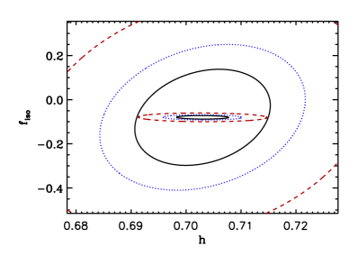
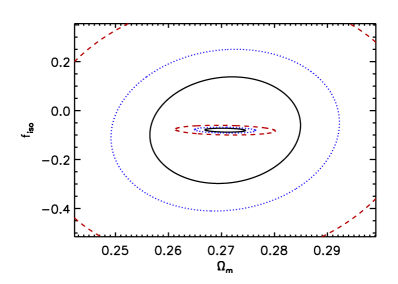
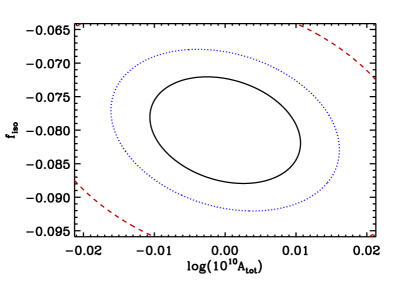
Figure 1: 2-parameter confidence levels for $f_{iso}$ and $q_{\alpha}$ with $q_{\alpha}=h,\Omega_{b},\Omega_{m},\log(10^{10}\,A_{\rm tot})$ for the fiducial model with $f_{iso}=-0.08$ obtained for an Euclid-like survey only (larger contours) and after combining the survey data with Planck. For $\log(10^{10}\,A_{\rm tot})$ we show the constraints from LSS+CMB only since for the LSS alone, using the $P(k)$-method, we marginalize over the power spectrum normalization. The blue dotted line and the red dashed line represent the 68$\%$ C.L., 95.4$\%$ C.L., respectively. The black solid line shows the 1-parameter confidence level at 1–$\sigma$.

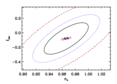
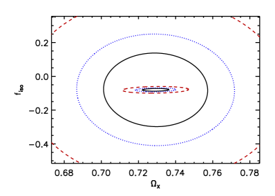
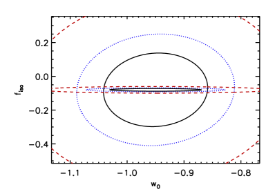
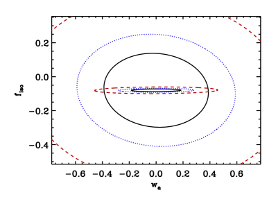
Figure 2: 2-parameter confidence levels for $f_{iso}$ and $q_{\alpha}$ with $q_{\alpha}=n_{s},\Omega_{X0},w_{0},w_{a}$ for the fiducial model with $f_{iso}=-0.08$ obtained for an Euclid-like survey only (larger contours) and after combining the survey data with Planck. The blue dotted line and the red dashed line represent the 68$\%$ C.L., 95.4$\%$ C.L., respectively. The black solid line shows the 1-parameter confidence level at 1–$\sigma$.

LSS+CMB
$q_{\alpha}$	$\hat{q}_{\alpha}$	$\sigma(q_{\alpha})$	$r(q_{\alpha}$)	$\frac{\delta\theta_{\alpha}}{\delta f_{iso}}|_{\delta f_{iso}=1}$	$\frac{\delta\theta_{\alpha}}{\delta f_{iso}}|_{\delta f_{iso}=0.08}$	$\frac{\delta\theta_{\alpha}}{\delta f_{iso}}|_{\delta f_{iso}=0.01}$
$\Omega_{m_{0}}$	$0.2707$	0.00379	-0.165	$-0.0788$	$-0.00630$	$-0.000788$
$\Omega_{X_{0}}$	$0.7293$	0.00712	0.124	$0.1117$	$0.008939$	$0.00111$
$\Omega_{b_{0}}$	$0.0451$	0.00061	-0.014	$-0.00101$	$-8.793\,10^{-5}$	$-1.01\,10^{-5}$
$h$	$0.703$	0.0047	-0.054	$-0.0321$	$-0.00257$	$-0.000321$
$n_{s}$	$0.966$	0.00317	0.69	$0.2770$	$0.02216$	$0.00277$
$w_{0}$	$-0.95$	0.08349	-0.02	$-0.242$	$-0.0193$	$-0.00242$
$w_{a}$	$0$	0.18390	0.08	$1.9786$	$0.1583$	$0.019786$
$\log(10^{10}A_{\rm tot})$	$1.3909$	0.0106	-0.24	$-0.7471$	$-0.0597$	$-0.00747$
$f_{iso}$	$-0.08$	0.00794	1	$1$	$0.08$	$0.01$
LSS
$\Omega_{m_{0}}$	$0.2707$	0.01421	0.090	$0.00593$	$0.000474915$	$0.0000593$
$\Omega_{X_{0}}$	$0.7293$	0.02803	-0.018	$-0.00241$	$-0.000193233$	$-0.0024100$
$\Omega_{b_{0}}$	$0.0451$	0.00363	0.291	$0.00486$	$0.00038940$	$0.0000486$
$h$	$0.703$	0.0123	0.246	$0.01392$	$0.0011138$	$0.0001392$
$n_{s}$	$0.966$	0.0339	0.729	$0.11373$	$0.00909873$	$0.0011373$
$w_{0}$	$-0.95$	0.0914	0.060	$0.02551$	$0.00204113$	$0.0002551$
$w_{a}$	$0$	0.38839	-0.07	$-0.12471$	$-0.00997681$	$-0.0012471$
$f_{iso}$	$-0.08$	0.21771	1	$1$	$0.08$	$0.01$

Table 2: Forecast 1–$\sigma$ errors of the cosmological parameters $q_{\alpha}$ considered in the text and corresponding correlations with $f_{iso}$, for an Euclid-like experiment alone and in combination with Planck. In particular, in the 2^nd column we report the fiducial values adopted for the parameters listed in the 1^st column. The corresponding 1–$\sigma$ errors are reported in the 3^rd column, and the $q_{\alpha}$–$f_{iso}$ correlation coefficients in the 4^th column. Finally, in the 5^th, 6^th and 7^th columns we list the shifts of the parameters $\theta_{\alpha}$ for $\delta f_{iso}=1,0.08,0.01$, respectively.

In this work we consider a cosmological model with curvature, isocurvature and varying dark energy. In this case, the combination of a Planck-like CMB experiment and a LSS probe improves the constraints on the cosmological parameters by at least one order of magnitude with respect to the Planck-only constraints for a less general model with curvature and isocurvature but with a cosmological constant (see e.g. [36]).

Here, we have extended the analysis of Ref. [39] to the more general model described in §3, and, moreover, we have added the cosmological information from the LSS to the CMB-only constraints. The results are summarized in the first three columns of Tab. 2. Note that the 1-$\sigma$ error on $f_{iso}$ obtained from the joint CMB+LSS analysis is $\simeq 0.008$; this is slightly better than the error expected from Planck alone, $\sigma({f_{iso}})=0.01$ of Ref. [39], where $\Omega_{k}=0$ and $w=-1$ (both kept as fixed parameters) were assumed.

In Figs. 1-2 we show the contours at 68% CL, 95% CL and 1-parameter CL at 1–$\sigma$, for $f_{iso}$ and $q_{\alpha}$ with $q_{\alpha}=\{n_{s},\Omega_{X0},w_{0},w_{a},h,\Omega_{b},\Omega_{m},\log(10^{10}\,A_{\rm tot})\}$, for the fiducial model with $f_{iso}=-0.08$, obtained from an Euclid-like survey alone (larger contours), and from the combination with Planck data. For $\log(10^{10}\,A_{\rm tot})$ we show only the constraints from LSS+CMB, since for the LSS alone, using the $P(k)$-method, we marginalize over the power spectrum normalization.

From Figs. 1-2 and column 3 of Tab. 2 it is evident that the CMB+LSS constraints improve dramatically with respect to the LSS-only case and also with respect to the CMB-only case [39, 36]. This means that adding LSS is a powerful tool which allows to break the strong degeneracies that affect CMB measurements when curvature, isocurvature and varying dark energy are included in the analysis. As a consequence, constraints on the nature of the initial conditions are greatly improved by the combination CMB+LSS, with respect to CMB alone.

The next issue we address regards possible systematic errors on cosmological parameters due to incorrect assumptions about the nature of the initial conditions.

To this purpose, we calculate the shifts on the cosmological parameters due to an incorrect amount of the isocurvature fraction $f_{iso}$ in the fiducial model.

The results are summarized in the last three columns of Tab. 2. As can be noticed, the absolute shifts (see Eq. (29)) $\delta\theta_{\alpha}/\delta f_{iso}$ assume the largest values for the dark energy parameters $\Omega_{X_{0}}$, $w_{0}$, $w_{a}$, for the spectral index $n_{s}$, and for the amplitude $A_{\rm tot}$ (see the $4^{th}$ column in Tab. 2).

In interpreting these results one must bear in mind that, rather than the shifts themeselves, it is important to determine if and in which cases these shifts on cosmological parameters are larger than the corresponding statistical errors ($3^{rd}$ column in Tab. 2).

We have assumed a fiducial value $f_{iso}=-0.08$, so, if the true underlying model were adiabatic (for which the“true” value for the isocurvature fraction is $f_{iso}=0$), $f_{iso}$ would be fixed to an incorrect value by $\delta f_{iso}=+0.08$. In this case, the correspondent shifts on the cosmological parameters are shown in the $5^{th}$ column of Tab. 2. For $\Omega_{m_{0}}$, $\Omega_{X_{0}}$, $A_{\rm tot}$ and $n_{s}$ (this last being the most affected parameter) the shifts are bigger than the 1–$\sigma$ statistical errors, meaning that the corresponding degeneracies with $f_{iso}$ are not completly solved, and a wrong assumption on the amount of isocurvature perturbations produces a bias in the estimation of the cosmological parameters even when adding LSS to CMB. On the other hand, the shift is slightly smaller but still comparable to the 1–$\sigma$ error for $w_{a}$. For the case $\delta f_{iso}=+0.08$, adding the LSS information breaks the degeneracy $f_{iso}$-$h$ with respect to the CMB-only case, even if the $h$-shift is still comparable to the statistical error. For the other parameters the degeneracies are reduced and the shifts are smaller but still of the same order of magnitude as the statistical 1–$\sigma$ errors.

On the other hand, if we consider the smaller value $\delta f_{iso}=+0.01$, the LSS information from an Euclid-like survey solves the degeneracies with $f_{iso}$ for all the cosmological parameters except $n_{s}$, as shown in the $6^{th}$ column of Tab. 2. This is a remarkable result given that the analysis is done including curvature and a varying dark energy equation of state.

Since the statistical errors are not very sensitive to the fiducial $f_{iso}$ value, the case $\delta f_{iso}=+0.01$ is representative to quantify the difference in modeling with the pure adiabatic case and the mixed underlying model with a fiducial $f_{iso}=-0.01$.

As shown in Figs. 1-2, for CMB+LSS the constraints on parameters which are degenerate with $f_{iso}$ improve considerably. However, note that the shifts on parameters as $\Omega_{X}$, $\Omega_{m0}$, $w_{0}$ and $w_{a}$ are larger than in the LSS-only case, as shown in column 5 of Tab. 2.

This is confirmed by the behavior of the correlation coefficient $r$ (see Eq. (28)), shown in column 4 of Tab. 2. For instance, if we consider the correlation $f_{iso}$-$\Omega_{X_{0}}$, we can observe that $f_{iso}$ and $\Omega_{X_{0}}$ are negligibly correlated for LSS measurements, but they are tightly correlated for CMB measurements; when combining the two information, the LSS help to alleviate the degeneracy but a level of correlation still remains.

In some cases the correlation coefficient $r$, as well as the shifts, can even change sign when adding Planck to LSS. This change follows the dominant correlations between $f_{iso}$ and the cosmological parameters either from LSS or CMB.

The parameter for which the degeneracy with the isocurvature fraction parameter $f_{iso}$ is not solved even when combining the CMB and LSS information is the spectral index $n_{s}$. We interpret this as due in part to the fact that in this paper we assume a curvaton underlying model as a working example for which $n_{s}\equiv n_{ad}=n_{iso}$. Therefore, $n_{s}$ encodes the information of both the spectral indices which are correlated with $f_{iso}$ for both CMB and LSS. In fact, the effect of a variation of $n_{iso}$ on the $C_{l}$ and the $P(k)$ would be different even for a fixed $f_{iso}$. Conversely, the effect of changing $f_{iso}$ would be different in CMB and LSS if $n_{ad}$ were not to be equal to $n_{iso}$. For the current data, the effect of changing $f_{iso}$ is stronger in CMB which thus “dominates” over LSS. Therefore, the magnitude of the degeneracy $n_{s}-f_{iso}$ is related to our choice $n_{s}\equiv n_{ad}=n_{iso}$. When $n_{iso}=n_{ad}$ the information is compressed in one parameter which in some way is “double-degenerate” with $f_{iso}$ and adding LSS helps but not enough to fully solve the degeneracy.

These results confirm once again the great potential of forthcoming large scale galaxy surveys.

5 Discussion and conclusions

In this work we have relied on the Fisher matrix approach to forecasts, which is not well suited to quantify systematic effects. The errors we have reported are statistical only, which are optimistic in the sense that we assume that systematic errors are vastly sub-dominant. Let us therefore discuss sources of systematic errors of major concern and their possible consequences on our results: these are the effects of non-linearities and galaxy bias.

In the analysis presented here we have used the linear theory matter power spectrum and a scale-independent galaxy bias. Our choice of the maximum k-mode ensures that the effects of non-linearity are quite mild and that eventually, before an analysis is performed on real data, they could be accurately modeled. Having considered only the mildly non-linear regime ensures that non-linearities will not erase or reduce significantly the signal. Reconstruction techniques that are being developed [71, 72] and/or are already being applied to surveys [73] offer promising prospects. Thus while it will be mandatory to include non-linearities in the actual data analysis, the forecasted errors are not made artificially smaller by using the linear matter power spectrum to compute our Fisher matrices.

Including smaller, more non-linear scales might help to improve the errors but would worsen the systematic effect of non-linearities and of a possible scale-dependent and/or non-linear bias. In this work we have made the simplifying assumption that bias is scale-independent but that the redshift dependence is not well known and so it is marginalised over. Bias is known to be scale-independent on large scales but scale dependent for small scales and/or very massive halos. While halo bias can be modeled, the bias of galaxies hosted in dark matter halos can be more complicated especially at small scales. Here we have considered scales where the so-called two halo term dominates and so complicated bias arising from the details of galaxy formation and halo occupation distributions do not matter. In addition we have checked that most of the information, useful to break degeneracies between the sound horizon at radiation drag and isocurvature contribution, come mostly from very large scales (those constraining the matter -radiation equality). The BAO signal is localized on scales where scale-dependent bias is more likely to be an issue, but the BAO location is relatively robust to this. Our reported error-bars could have been made smaller by considering also information about the growth of structures (i.e., redshift space distortions and the normalization of the power spectrum), however we decided to, conservatively, marginalise over the amplitude to be less sensitive to possible assumptions about galaxy bias.

As found in Ref. [39] for a Planck-like CMB experiment, even a tiny isocurvature fraction contribution, if not accounted for, can lead to an incorrect determination of the cosmological parameters even for a standard flat model with a cosmological constant. In this case however, when the isocurvature parameter $f_{iso}$ is added to the modelling, the errors increase but the cosmological parameters are recovered correctly. The error degradation from a CMB-only analysis is particularly severe for models where spatial flatness is not imposed and curvature is left as a free parameter.

In this work we extend the analysis done in Ref. [39] and present the results from a joint analysis of a CMB Planck-like experiment and a LSS EULID-like galaxy survey, for a cosmological model that includes an isocurvature fraction in the initial conditions, varying dark energy and curvature.

As shown in Figs. 1-2 and in Tab. 2, we find that adding the cosmological information coming from an Euclid-like LSS probe strongly reduces the degeneracies introduced by the presence of an isocurvature contribution with respect to a Planck-like CMB probe alone.

When isocurvature is included in the analysis, we find that the most affected parameter is the spectral index $n_{s}$ for which the degeneracy with the isocurvature fraction parameter $f_{iso}$ is never fully solved even when combining CMB and LSS. This is because in this paper we assume a curvaton underlying model as a working example for which $n_{s}\equiv n_{ad}=n_{iso}$. Therefore $n_{s}$ encodes the information of both the spectral indices which are correlated with $f_{iso}$ for both CMB and LSS. In this case, from the combination CMB+LSS, we find an absolute $n_{s}$-shift$=0.277$ which is larger than the statistical 1–$\sigma$ error by two order of magnitude. For all the cosmological parameters the correlations with $f_{iso}$ and the corresponding shifts are reported in Tab. 2. Our findings are quantitative only for the $n_{ad}=n_{iso}$ case, but can hold qualitatively for other models with $n_{iso}\simeq 1$, as for example the axion-like isocurvature model. In this case, since $n_{ad}$ is close to scale invariant, we expect that the effect will be quantitatively very similar.

We investigate also the effect on the recovered cosmological parameters in the case of the presence of a small amount of isocurvature which is however ignored in the analysis. Ref. [39] found that even a tiny isocurvature fraction, if neglected, could bias the determination of “standard rulers” like the sound horizon $r_{s}(z_{d})$ at radiation drag and introduce systematic biases in the interpretation of BAO observables that are larger than the statistical error-bars forecast for future and forthcoming surveys. Ref. [39] considered a flat Universe where the dark energy is a cosmological constant, but in a more general cosmology the effect can be dramatically worst.

Here we find that adding LSS information to CMB priors eliminates the bias (i.e. reduces it well below the statistical errors) in the case of a small amount of isocurvature fraction $f_{iso}\sim{\cal O}(10^{-2})$, even for a general cosmological model with varying dark energy and curvature. The only parameter for which the systematic shift remains still comparable to the 1–$\sigma$ error is the spectral index $n_{s}$.

These remarkable results are obtained by better exploiting the potential cosmological information of future LSS surveys by adding to BAO measurements also the power spectrum shape, following the so-called $P(k)$-method marginalised over growth information. In fact, the additional cosmological information in the power spectrum helps to break degeneracies among the cosmological parameters, and thus indirectly improves the constraints on the isocurvature parameter $f_{iso}$.

Considering that -conservatively- we have not included information on the power spectrum amplitude and on the growth of cosmological structures (we marginalize over redshift space distortions parameters and LSS power spectrum normalization), we conclude highlighting once again the synergy and complementarity between CMB and LSS and the great potential of future galaxy surveys.

Appendix A Planck Fisher matrix

In this work we use the Planck mission parameter constraints as CMB priors, by estimating the cosmological parameter errors via measurements of the temperature and polarization power spectra. As CMB anisotropies, with the exception of the integrated Sachs-Wolfe effect, are not able to constrain the equation of state of dark energy $(w_{0},w_{a})$, we follow the prescription laid out by DETF [56].

We do not include any B-mode in our forecasts and assume no tensor mode contribution to the power spectra. We use the 100 GHz, 143 GHz, and 217 GHz channels as science channels. These channels have a beam of $\theta_{\rm fwhm}=9.5^{\prime}$, $\theta_{\rm fwhm}=7.1^{\prime}$, and $\theta_{\rm fwhm}=5^{\prime}$, respectively, and sensitivities of $\sigma_{T}=2.5\mu K/K$, $\sigma_{T}=2.2\mu K/K$, $\sigma_{T}=4.8\mu K/K$ for temperature, and $\sigma_{P}=4\mu K/K$, $\sigma_{P}=4.2\mu K/K$, $\sigma_{P}=9.8\mu K/K$ for polarization, respectively. We take $f_{\rm sky}=0.80$ as the sky fraction in order to account for galactic obstruction, and use a minimum $\ell$-mode $\ell_{\rm min}=30$ in order to avoid problems with polarization foregrounds and not to include information from the late Integrated Sachs-Wolfe effect, which depends on the specific dark energy model. We discard temperature and polarization data at $\ell>2000$ to reduce sensitivity to contributions from patchy reionization and point source contamination (see [56] and references therein).

We assume a fiducial cosmology with an anti-correlated isocurvature contribution, varying dark energy and curvature. Therefore we choose the following set of parameters to describe the temperature and polarization power spectra $\vec{\theta}=(\omega_{m},\omega_{b},f_{iso},100\times\theta_{S},\log(10^{10}A_{\rm tot}),n_{S},w_{0},w_{a})$, where $\theta_{S}$ is the angular size of the sound horizon at last scattering and $w_{0}$ and $w_{a}$ are the dark energy parameters according to the CPL parametrization of the dark energy equation of state $w(z)=w_{0}+w_{a}\,z/(1+z)$.

The Fisher matrix for CMB power spectrum is given by [74, 75]:

$$F_{ij}^{CMB-Planck}=\sum_{l}\sum_{X,Y}\frac{\partial C_{X,l}}{\partial\theta_{i}}\mathrm{COV^{-1}_{XY}}\frac{\partial C_{Y,l}}{\partial\theta_{j}},$$ (30)

where $\theta_{i}$ are the parameters to constrain, $C_{X,l}$ is the harmonic power spectrum for the temperature-temperature ($X\equiv TT$), temperature-E-polarization ($X\equiv TE$) and the E-polarization-E-polarization ($X\equiv EE$) power spectrum. The covariance $\rm{COV}^{-1}_{XY}$ of the errors for the various power spectra is given by the fourth moment of the distribution, which under Gaussian assumptions is entirely given in terms of the $C_{X,l}$ with

$${\rm COV}_{T,T} = f_{\ell}\left(C_{T,l}+W_{T}^{-1}B_{l}^{-2}\right)^{2}$$ (31)

$${\rm COV}_{E,E} = f_{\ell}\left(C_{E,l}+W_{P}^{-1}B_{l}^{-2}\right)^{2}$$ (32)

$${\rm COV}_{TE,TE} = f_{\ell}\Big{[}C_{TE,l}^{2}+\left(C_{T,l}+W_{T}^{-1}B_{l}^{-2}\right)\left(C_{E,l}+W_{P}^{-1}B_{l}^{-2}\right)\Big{]}$$ (33)

$${\rm COV}_{T,E} = f_{\ell}C_{TE,l}^{2}$$ (34)

$${\rm COV}_{T,TE} = f_{\ell}C_{TE,l}\left(C_{T,l}+W_{T}^{-1}B_{l}^{-2}\right)$$ (35)

$${\rm COV}_{E,TE} = f_{\ell}C_{TE,l}\left(C_{E,l}+W_{P}^{-1}B_{l}^{-2}\right)\;,$$ (36)

where $f_{\ell}=2/((2\ell+1)f_{\rm sky})$, $W_{T,P}=\sum_{c}W^{c}_{T,P}$, $W^{c}_{T,P}=(\sigma^{c}_{T,P}\theta^{c}_{\rm fwhm})^{-2}$ being the weight per solid angle for temperature and polarization respectively, with a 1–$\sigma$ sensitivity per pixel of $\sigma^{c}_{T,P}$ and a beam of $\theta^{c}_{\rm fwhm}$ extent, for each frequency channel $c$. The beam window function is given in terms of the full width half maximum (fwhm) beam width by $B_{\ell}^{2}=\sum_{c}(B^{c}_{\ell})^{2}W^{c}_{T,P}/W_{T,P}$, where $(B^{c}_{\ell})^{2}=\exp\left(-\ell(\ell+1)/(l^{c}_{s})^{2}\right)$, $l^{c}_{s}=(\theta^{c}_{\rm fwhm})^{-1}\sqrt{(}8\ln 2)$ and $f_{\rm sky}$ is the sky fraction [76].

We then calculate the Planck CMB Fisher matrix with the help of the publicly available CAMB code [77]. Finally, we transform the Planck Fisher matrix for the DETF parameter set to the final parameter sets $\bf q$ considered in this work (see §3), using the transformation

$$F_{\alpha\beta}^{CMB-Planck}=\sum_{ij}\frac{\partial\theta_{i}}{\partial q_{\alpha}}\,F_{ij}^{CMB-Planck}\,\frac{\partial\theta_{j}}{\partial q_{\beta}}.$$ (37)

References

- [1] V. Mukhanov, H.A. Feldman and R.H. Brandenberger, Phys. Rept. 15, 203 (1992).
- [2] Brandenberger, R., Mukhanov, V., & Prokopec, T. 1992, Physical Review Letters, 69, 3606
- [3] Komatsu, E., et al. 2010, \arXivid1001.4538
- [4] A. D. Linde, Phys. Lett. B 158, 375 (1985); A. D. Linde and V. Mukhanov, Phys. Rev. D 56, 535 (1997);
- [5] L. A. Kofman and A. D. Linde, Nucl. Phys. B 282, 555 (1987);
- [6] S. Mollerach, Phys. Lett. B 242, 158 (1990);
- [7] D. Polarski and A. A. Starobinsky, Phys. Rev. D 50, 6123 (1994); M. Sasaki and E. D. Stewart, Prog. Theor. Phys. 95, 71 (1996); M. Sasaki and T. Tanaka, Prog. Theor. Phys. 99, 763 (1998).
- [8] Langlois, D., PhysRevD.59, 123512 (1999)
- [9] P. J. E. Peebles, Astrophys. J. 510, 523 (1999).
- [10] N. Bartolo, S. Matarrese and A. Riotto, Phys. Rev. D 64, 123504 (2001); C. Gordon, D. Wands, B. A. Bassett and R. Maartens, Phys. Rev. D 63, 023506 (2001); D. Wands, N. Bartolo, S. Matarrese and A. Riotto, Phys. Rev. D 66, 043520 (2002). J. García-Bellido and D. Wands, Phys. Rev. D 53, 5437 (1996); 52, 6739 (1995).
- [11] M. Bucher&al. Phys. Rev. D 62, 083508 (2000)
- [12] M. Axenides, R. H. Brandenberger and M. S. Turner, Phys. Lett. B 126 (1983) 178.
- [13] A. D. Linde, JETP Lett. 40 (1984) 1333 [Pisma Zh. Eksp. Teor. Fiz. 40 (1984) 496]; Phys. Lett. B 158, 375 (1985); Phys. Lett. B 201 (1988) 437.
- [14] D. Seckel and M. S. Turner, Phys. Rev. D 32 (1985) 3178.
- [15] A. D. Linde, Phys. Lett. B 259 (1991) 38.
- [16] M. S. Turner and F. Wilczek, Phys. Rev. Lett. 66 (1991) 5.
- [17] A. D. Linde and D. H. Lyth, Phys. Lett. B 246 (1990) 353.
- [18] D. H. Lyth, Phys. Rev. D 45 (1992) 3394.
- [19] E. P. S. Shellard and R. A. Battye, \arXividastro-ph/9802216.
- [20] M. Kawasaki, N. Sugiyama and T. Yanagida, Phys. Rev. D 54, 2442 (1996);
- [21] A. D. Linde and V. F. Mukhanov, Phys. Rev. D56, 535 (1997), \arXividastro-ph/9610219
- [22] D. H. Lyth and D. Wands, Phys. Lett.B 524, 5-14 (2002).
- [23] D. H. Lyth, C. Ungarelli, and D. Wands, Physical Review D 67, 023503 (2003).
- [24] G. Efstathiou and J.R. Bond, “Isocurvature cold dark matter fluctuations” MNRS 218, 103 (1986)
- [25] K. Enqvist, H. Kurki-Suonio and J. Valiviita, Phys. Rev. D 65, 043002 (2002)
- [26] L. Page et al. Astrophys. J. Suppl. 148 233 (2003)
- [27] G. Hinshaw et al. Astrophys. J. Suppl.170 288 (2007)
- [28] Maria Beltran, Juan Garcia-Bellido, Julien Lesgourgues, Alain Riazuelo Journal-ref: Phys.Rev. D70 (2004) 103530
- [29] Maria Beltran, Juan Garcia-Bellido, Julien Lesgourgues, Matteo Viel Phys.Rev.D72:103515,2005
- [30] J. Valiviita and T. Giannantonio, Phys. Rev. D 80, 123516 (2009)
- [31] J. Dunkley et al., Phys. Rev. Lett. 95, 261303 (2005)
- [32] Keskitalo, R., Kurki-Suonio, H., Muhonen, V., Valiviita, J. 2007, Journal of Cosmology and Astro-Particle Physics, 9, 8
- [33] J. Valiviita and V. Muhonen, Phys. Rev. Lett. 91, 131302 (2003)
- [34] R. Trotta New Astron. Rev. 47, 769-774 (2003)
- [35] D. Langlois and A. Riazuelo Phys. Rev. D 62, 043504 (2000)
- [36] M. Bucher, K. Moodley and N. Turok, Cosmology and Particle Physics, 555, 313 (2001)
- [37] Sollom, I., Challinor,A., & Hobson, M. P. 2009, Phys. Rev. D , (7) 9, 123521
- [38] M. Bucher, K. Moodley and N. Turok, Physical Review Lett 87, 191301 (2001).
- [39] A. Mangilli, L.Verde and M.Beltran, JCAP 10 009 (2010), \arXivid1006.3806
- [40] H.Kurki-Suonio, V. Muhonen and J. Valiviita Phys. Rev. D 71, 063005 (2005)
- [41] C. Carbone, L. Verde, Y. Wang and A. Cimatti, JCAP03 030 (2011)
- [42] W. Hu, D.N. Spergel and M. White, Phys.Rev. D 55, 3288-3302 (1997)
- [43] H.V. Peiris et al., “First-Year Wilkinson Microwave Anisotropy Probe (WMAP) Observations: Implications For Inflation” Astophys. J. Suppl. 148, 213 (2003)
- [44] Komatsu, E., et al. 2009, Astrophys. J. Suppl., 180, 330
- [45] D. Larson Astrophys.J.Suppl. 192 16 (2011)
- [46] R.A. Fisher, J. Roy. Stat. Soc., 98, 39 (1935)
- [47] R. Laureijs, et al. (Euclid Science Study Team), \arXivid0912.0914
- [48] Feldman, H., A., Kaiser, N., & Peacock, J., A. 1994, Astrophys. J., 426, 23
- [49] M. Chevallier and D. Polarski, Int. J. Mod. Phys. D 10, 213 (2001).
- [50] E. V. Linder, Phys. Rev. Lett. 90, 091301 (2003).
- [51] Vogeley, M. S. & Szalay, A. S. 1996 Astrophys. J., 465, 43
- [52] Tegmark, M., Taylor A., Heavens A. 1997, Astrophys. J., 480, 22
- [53] Jungman, G., Kamionkowski, M., Kosowsky, A., Spergel, D. 1996, Phys. Rev. D, 54, 1332
- [54] Seo, H., J., & Eisenstein, D., J. 2003, Astrophys. J., 598, 720
- [55] Eisenstein, D. J., & Hu, W. 1998, ApJ, 496, 605
- [56] Albrecht, A., et al. 2006, \arXividastro-ph/0609591
- [57] W. E. Ballinger, J. A. Peacock, and A. F. Heavens, Mon.Not.Roy.As.Soc. 282, 877 (1996), a
- [58] Seljak, U. 2000, Mont. Not. Roy. Astron. Soc., 318, 203
- [59] Kaiser, N. 1987, Mont. Not. Roy. Astron. Soc., 227, 1
- [60] Linder, E. V. & Jenkins, A. 2003, Mont. Not. Roy. Astron. Soc., 346, 573
- [61] Lewis, A., Challinor, A., & Lasenby, A. 2000, Astrophys. J., 538, 473
- [62] Wang, Y. 2010, Mod. Phys. Lett. A, 25, 3093
- [63] Wang, Y. 2008, Journal of Cosmology and Astro-Particle Physics, 05, 021
- [64] Tegmark, S. 1997, Phys. Rev. Lett., 79, 3806
- [65] Wang, Y. 2006, Astrophys. J., 647, 1
- [66] A. F. Heavens, T.D. Kitching and L. Verde Mon. Not. Roy. Astron. Soc. 380,1029-1035 (2007)
- [67] Wang, Y. 2008, Phys. Rev. D, 77, 123525
- [68] Wang, Y., et al. 2010, Mont. Not. Roy. Astron. Soc., 409, 737
- [69] Geach, J. E.; Cimatti, A.; Percival, W.; Wang, Y.; Guzzo, L.; Zamorani, G.; Rosati, P.; Pozzetti, L.; Orsi, A.; Baugh, C. M.; Lacey, C. G.; Garilli, B.; Franzetti, P.; Walsh, J. R.; Kümmel, M., 2010, Mont. Not. Roy. Astron. Soc., 402, 1330
- [70] Orsi, Alvaro; Baugh, C. M.; Lacey, C. G.; Cimatti, A.; Wang, Y.; Zamorani, G., \arXivid0911.0669, Mont. Not. Roy. Astron. Soc., 402 1330G (2010)
- [71] Eisenstein, D. J., Seo, H.-J., Sirko, E., & Spergel, D. N. 2007, ApJ, 664, 675
- [72] Wagner, C., Müller, V., & Steinmetz, M. 2008, A&A, 487, 63
- [73] Reid, B. A., et al. 2010, MNRAS, 404, 60
- [74] Zaldarriaga M., Seljak U., 1997, PRD, 55, 1830
- [75] Zaldarriaga M., Spergel D. N., Seljak U., 1997, APJ, 488, 1
- [76] Bond, J. R., Efstathiou, G., & Tegmark, M. 1997 Mont. Not. Roy. Astron. Soc., 291, L33
- [77] Lewis, A., Challinor, A., & Lasenby, A. 2000, Astrophys. J., 538, 473