Real-Reward Testing for Probabilistic Processes
(Extended Abstract)
Yuxin Deng1
Rob van Glabbeek2
Matthew Hennessy3
Carroll Morgan4Deng was supported by the National Natural Science Foundation of China (61033002).Supported by SFI project SFI 06 IN.1 1898.Morgan acknowledges the support of ARC Discovery Grant DP0879529.1 Shanghai Jiao Tong University and Chinese Academy of Sciences, China2 National ICT Australia, Australia3 Trinity College Dublin, Ireland2,4 University of New South Wales, Australia
Abstract
We introduce a notion of real-valued reward testing for probabilistic
processes by extending the traditional nonnegative-reward testing with
negative rewards. In this richer testing framework, the may and must
preorders turn out to be inverses. We show that for convergent
processes with finitely many states and transitions, but not in the
presence of divergence, the real-reward must-testing preorder
coincides with the nonnegative-reward must-testing preorder. To prove
this coincidence we characterise the usual resolution-based testing in
terms of the weak transitions of processes, without having to involve
policies, adversaries, schedulers, resolutions, or similar structures
that are external to the process under investigation. This requires
establishing the continuity of our function for calculating testing
outcomes.
1 Introduction
Extending classical testing semantics [2, 8] to a
setting in which probability and nondeterminism co-exist was initiated
in [14]. The application of a test to a process yields a set
of probabilities for reaching a success state. Reward testing
was introduced in [9]; here the success states are labelled
by nonnegative real numbers—rewards—to indicate degrees of
success, and reaching a success state
accumulates the associated reward. In [13] an infinite set of
success actions is used to report success, and the testing
outcomes are vectors of probabilities of performing these success
actions. Compared to [9] this amounts to distinguishing
different qualities of success, rather than different quantities.
In [14] and [13], both tests and testees are
nondeterministic probabilistic processes, whereas [9] allows
nonprobabilistic tests only, thereby obtaining a less discriminating
form of testing. In [7] we strengthened reward testing by also
allowing probabilistic tests. Taking rewards testing in this form we showed that for finitary
processes, i.e. finite-state and finitely branching processes, all
three modes of testing lead to the same testing preorders. Thus, vector-based testing is no more powerful than scalar testing that employs
only one success action, and likewise reward testing is no more
powerful than the special case of reward testing in which all rewards are 1.
111In spite of this there is a difference in power
between the notions of testing from [14] and [13], but
this is an issue that is entirely orthogonal to the distinction
between scalar testing, reward testing and vector-based testing. In
[13] it is the execution of a success action that
constitutes success, whereas in [2, 8, 14, 9] it is
reaching a success state (even though typically success actions
are used to identify those states). In [3, Ex 5.3] we showed
that state-based testing is (slightly) more powerful than action-based
testing. The results presented in [7] about the coincidence of
scalar, reward, and vector-based testing preorders pertain to
action-based version of each, but in the conclusion it is observed
that the same coincidence could be obtained for their state-based
versions. In the current paper we stick to state-based testing.
In certain situations it is natural to introduce negative rewards.
This is the case, for instance, in the theory of Markov Decision
Processes [10]. Intuitively, we could understand negative
rewards as costs, while positive rewards are often viewed as benefits
or profits. This leads to the question: if negative rewards are
also allowed, how would the original reward-testing semantics change?
We refer to the more relaxed form of testing, using positive and
negative rewards, as real-reward testing and the original one
(from [9], but with probabilistic tests as in [7]) as
nonnegative-reward testing.
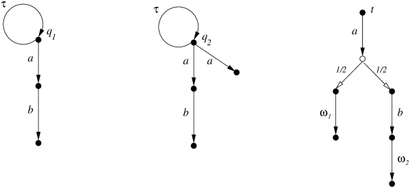
Figure 1: Two processes with divergence and a test
The power of real-reward testing is illustrated in Figure 1.
The two (nonprobabilistic) processes in the left- and central diagrams are equivalent under
(probabilistic) may- as well as must testing; the -loops in the
initial states cause both processes to fail any nontrivial must test. Yet, if a
reward of is associated with performing the action , and a
reward of with the subsequent performance of
(implemented by the test in the right diagram; see Example 3.8 for more details), in the first process the net
reward is either (if the process remains stuck in its initial
state) or positive, whereas running the second process may yield a
loss. This example shows that for processes that may exhibit
divergence, real-reward testing is more discriminating than
nonnegative-reward testing, or other forms of probabilistic testing.
It also illustrates that the extra power may be relevant in applications.
As remarked, in [7] we established that for finitary processes the
nonnegative-reward must-testing preorder () coincides
with the probabilistic must-testing preorder (), and
likewise for the may preorders.
Here we show that, in
contrast to the situation for nonnegative-reward (or scalar)
testing, for real-reward testing the may- and must preorders are the
inverse of each other, i.e. for any processes and ,
(1)
Our main result is that restricted to finitary convergent
processes, the real-reward must preorder coincides with the
nonnegative-reward must preorder, i.e. for any finitary convergent
processes , ,
(2)
Here by convergence we mean that
there is no infinite sequence of internal transitions
of the form with
distribution (and thus its successors) reachable from either or .
This rules out the processes of Figure 1.
Although it is easy to see that in (2) the former
implies the latter, to prove the opposite is far from trivial.
We employ a novel characterisation of
the usual resolution-based testing approach, without introducing concepts
like policy [10], adversary [11],
scheduler [12] or resolution [7] that are
external to the process under investigation; instead we describe the
mechanism for gathering test results in terms of the weak
-moves or derivations [4] the investigated
process can make, and hence speak of derivation-based testing.
This allows us to exploit the failure simulation preorder
that in [4] was proven to coincide with the
probabilistic must testing preorder based on resolutions,
at least for finitary processes.
Using the derivational characterisation we can show that, for
finitary convergent processes, is contained in .
Convergence is essential here, even though it is not needed to
establish that is contained in .
Combining this with the results from [7] and [4] mentioned above
leads to our required result that is included in
, as far as finitary convergent processes are
concerned. Consequently, in this case, all the relations of
Figure 2 collapse into one.
The symbol between two relations means that they
coincide for finitary convergent processes.
Figure 2: The relationship of different testing preorders.
The rest of this paper is organised as follows. We start by recalling
notation for probabilistic labelled transition systems. In
Section 3 we review the resolution-based testing
approach and show that the real-reward may preorder is simply the
inverse of the real-reward must preorder. Moreover, using the example
of Figure 1, we show that in the presence of divergence
the inclusion of in is proper. In
Section 4 we present the derivation-based testing approach
and also show that the two approaches agree.
Then in Section 5 we show
for finitary convergent processes that real-reward must testing
coincides with nonnegative-reward must testing.
We conclude in Section 6.
Due to lack of space, we omit all proofs: they are reported in
[5]. Besides the related work already mentioned above, many
other studies on probabilistic testing and simulation semantics
have appeared in the literature. They are reviewed in
[6, 3].
2 Probabilistic Processes
A (discrete) probability subdistribution over a set is a
function with ; the support of such a is
, and its
mass is
. A subdistribution is
a (total, or full) distribution if . The point
distribution assigns probability to and to all
other elements of , so that . With
we denote the set of subdistributions over , and with
its subset of full distributions.
Let be a set
of subdistributions, possibly infinite. Then is the
real-valued function in defined by
.
This is a partial operation on subdistributions because
for some state the sum of might exceed . If the
index set is finite, say , we often write . For a real
number from we use
to denote the subdistribution given by . Finally we use to denote the
everywhere-zero subdistribution that thus has empty support. These
operations on subdistributions do not readily adapt themselves to
distributions; yet if for
some , and the are distributions,
then so is .
The expected value over a
subdistribution of a bounded nonnegative function to the
reals or tuples of them is written , and the image of a
subdistribution through a function , for some set , is written
— the latter is the subdistribution over
given by for each .
Definition 2.1.
A probabilistic labelled transition system (pLTS) is a triple
, where
(i)
is a set of states,
(ii)
is a set of visible actions,
(iii)
relation is a subset of .
Here denotes , where
is the invisible- or internal action.
A (nonprobabilistic) labelled transition system (LTS) may be viewed
as a degenerate pLTS — one in which only point distributions are
used.
In this paper a (probabilistic) process will simply be a
distribution over the state set of a pLTS.
As with LTSs, we write for
, as well as
for and
for ,
with and representing their negations.
A pLTS is deterministic if for any state and
label there is at most one distribution with .
It is finitely branching if the set is finite for all states ;
if moreover is finite, then the pLTS is finitary.
A subdistribution over the state set of an arbitrary pLTS is finitary
if restricting to the states reachable from
yields a finitary sub-pLTS.
3 Testing probabilistic processes
A test is a distribution over the state set of a pLTS having
as its set of transition labels, where is a
set of fresh success actions, not already in , introduced specifically to
report testing outcomes.222For vector-based testing we
normally take to be countably infinite [13]. This
way we have an unbounded supply of success actions for
building tests, of course without obligation to use them all.
Scalar testing is obtained by taking .
For simplicity we may assume a fixed pLTS of
processes—our results apply to any choice of such a pLTS—and a
fixed pLTS of tests. Since the power of testing depends on the expressivity
of the pLTS of tests—in particular certain types of tests are
necessary for our results—let us just postulate that this pLTS is sufficiently expressive
for our purposes — for example that it can be used to interpret all
processes from the language , as in our previous papers
[6, 3, 4].
Although we use success actions, they are used merely to mark
certain states as success states, namely the sources of transitions labelled by success
actions. For this reason we systematically ignore
the distributions that can be reached after a success action.
We impose two requirements on all states in a pLTS of tests, namely
(A)
if and with
then .
(B)
if with and with
then for all .
The first condition says that a success state can have one success
identity only, whereas the second condition is slight weakening
of the requirement from [9] that success states must be end
states; it allows further progress from an -success state, for
some , but must remain enabled.
333Justification for imposing such restrictions can be found in Appendix A of [7].
To apply test to process we form a parallel
composition in which all visible actions
of must synchronise with . The synchronisations are
immediately renamed into . The resulting composition is a
process whose only possible actions are the elements of . Formally, if and are the pLTSs of processes and
tests, then the pLTS of applications of tests to processes is , with and the
transition relation generated by the rules in Fig. 3.
Here if and ,
then is the distribution given by .
The resulting pLTS also satisfies (A), (B) above;
this would not be the case if we had strengthened
(B) to require that success states must be end states.
Figure 3: Synchronous parallel composition between tests and processes
We will define the result of applying the test
to the process to be a set of testing outcomes, exactly
one of which results from each resolution of the choices in .
Each testing outcome is
an -tuple of real numbers in the interval
[0,1], i.e. a function , and its
-component , for , gives the
probability that the resolution in question will reach an
-success state, one in which the success action
is possible.
Due to the presence of nondeterminism in pLTSs, we need a mechanism to
reduce a nondeterministic structure into a set of deterministic
structures, each of which determines a single possible outcome. Here we adapt
the notion of resolution, defined in [7] for
probabilistic automata, to pLTSs.
Definition 3.1.
[Resolution]
A resolution of a subdistribution in a
pLTS is a triple
where
is a deterministic pLTS and
, such that there exists a
resolving function satisfying
(i)
(ii)
if for
then
(iii)
if for then .
The reader is referred to Section 2 of [7] for a detailed
discussion of the concept of resolution, and the manner in which a
resolution represents a run of a process; in particular in a
resolution states in are allowed to be resolved into distributions,
and computation steps can be probabilistically interpolated.
Our resolutions match the results of applying a scheduler as defined
in [12].
We now explain how to associate an outcome with a particular
resolution, which in turn will associate a set of outcomes with a
subdistribution in a pLTS. Given a deterministic pLTS consider the functional
defined by
(3)
We view the unit interval ordered in
the standard manner as a complete lattice;
this induces the structure of a complete lattice on the product and in turn
on the set of functions
. The functional is easily seen to be
monotonic and therefore has a least fixed point, which we denote by
; this is abbreviated to when the
deterministic pLTS in question is understood.
Now we define to be the set of vectors
(4)
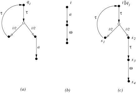
Figure 4: Testing the process
Example 3.2.
Consider the process
depicted in Figure 4(a). Here states are
represented by filled nodes and distributions by open nodes .
We leave out point-distributions — diverting an incoming
edge to the unique state in its support.
When we apply the test
depicted in Figure 4(b) to it we get the process
depicted in Figure 4(c).
This process is already deterministic, hence has essentially only one resolution: itself.
Moreover the outcome associated with it is
the least solution of the equation
where is the -tuple
with and for all
.
In fact this equation has a unique solution in , namely .
Thus .
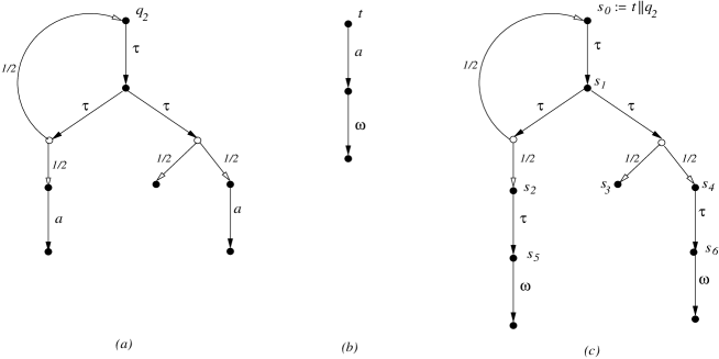
Example 3.3.
Consider the process
and the application of the test to it, as
outlined in Figure 5.
For each the process has a resolution
such that
; intuitively it goes around
the loop times before at last taking the right hand
action. Thus contains for
every . But it also contains , because of the
resolution which takes the left hand -move every time. Thus
includes the set
As resolutions allow any interpolation between the two -transitions
from state ,
is actually the convex closure of the above set.
Figure 5: Testing the process
There are two standard methods for comparing two sets of ordered outcomes:
if for every there exists some such that
if for every there exists some such that
This gives us our definition of the probabilistic may- and must-testing preorders;
they are decorated with for
the repertoire of testing actions they employ.
Definition 3.4.
[Probabilistic testing preorders]
(i)
if for every -test , .
(ii)
if for every -test , .
These preorders are abbreviated to and when .
In [7] we established that for finitary processes
coincides with and with for any
choice of . We also defined the reward testing preorders in
terms of the mechanism set up so far. The idea is to associate with
each success action a reward, which is a nonnegative
number in the unit interval ; and then a run of a probabilistic
process in parallel with a test yields an expected reward accumulated
by those states which can enable success actions. A reward tuple is used to assign reward to success action
, for each .
Due to the presence of nondeterminism, the application of a test
to a process produces a set of expected rewards.
Two sets of rewards can be compared by examining their suprema/infima; this gives
us two methods of testing called reward may/must testing. In
[7] all rewards are required to be nonnegative, so we refer to
that approach of testing as nonnegative-reward testing. If we
also allow negative rewards, which intuitively can be understood as
costs, then we obtain an approach of testing called real-reward
testing. Technically, we simply let reward tuples range over
the set . If , we use the
dot-product . It can apply to a set so that
. Let . We use
the notation for the supremum of set , and for the infimum.
Definition 3.5.
[Reward testing preorders]
(i)
if for every -test and nonnegative-reward tuple ,
.
(ii)
if for every -test and nonnegative-reward tuple ,
.
(iii)
if for every -test and real-reward tuple ,
.
(iv)
if for every -test and real-reward tuple ,
.
This time we drop the superscript iff is countably infinite.
It is shown in Corollary 1 of [7] that nonnegative-reward testing is equally powerful as probabilistic testing.
In this paper we focus on the real-reward testing preorders
and , by comparing them with the nonnegative
reward testing preorders and .
Although these two nonnegative-reward testing preorders are in
general incomparable we have:
Theorem 3.7.
For any processes and , it holds that
if and only if .
Our next task is to compare with . The former
is included in the latter, which directly follows from
Definition 3.5. Surprisingly, it turns out that for
finitary convergent processes the latter is also included in the
former, thus establishing that the two preorders are in fact the same. The rest of the
paper is devoted to proving this result. However, we first show that
this result does not extend to divergent processes.
Example 3.8.
Consider the processes and depicted in Figure 1.
Using the characterisations of and in [4],
it is easy to see that these processes cannot be distinguished by
probabilistic may- and must testing, and hence not by nonnegative-reward testing either.
However, let be the test in the right diagram of Figure 1 that first synchronises on the action
, and then with probability reaches a state in which a reward
of is allocated, and with the remaining probability
synchronises with the action and reaches a state that yields a reward of .
Thus the test employs two success actions and , and we use
the reward tuple with and .
Then the resolution of that does not involve the
-loop contributes the value
to the set , whereas the
resolution that only involves the -loop contributes the value .
Due to interpolation, is in fact
the entire interval . On the other hand, the resolution
corresponding to the -branch of contributes the value and
.
Thus
,
and hence .
4 Derivation-based testing
In this section we give an alternative definition of .
Our definition has four ingredients. First of all, for technical reasons we normalise our
pLTS of applications of tests to processes by
pruning away all outgoing -transitions from success states. This
way an -success state will only have outgoing transitions
labelled .
Definition 4.1.
[-respecting] A pLTS
is said to be -respecting whenever , for
any , implies .
It is straightforward to modify the pLTS of applications of tests to
processes into one that it is -respecting, namely by removing
all transitions for states with .
With we denote the distribution
in this pruned pLTS.
Secondly, we recall the definition of weak derivations from [4].
In a pLTS actions are only performed by states, in that actions are
given by relations from states to distributions. But processes
in general correspond to distributions over states, so in order to
define what it means for a process to perform an action, we need to
lift these relations so that they also apply to
distributions. In fact we will find it convenient to lift them to
subdistributions.
Definition 4.2.
Let be a pLTS and be a relation from states to subdistributions.
Then
is the smallest relation that satisfies:
(i)
implies , and
(ii)
(Linearity)
for implies
for any () with .
An application of this notion is when the relation is
for ; in that case we also write
for . Thus, as source of a relation we
now also allow distributions, and even subdistributions.
A subtlety of this approach is that for any action , we have
simply by taking or in
Definition 4.2. That turns out to make especially useful for
modelling the “chaotic” aspects of divergence in [4], in
particular that in the must-case a divergent process can simulate any
other.
Definition 4.3.
[Weak derivation]
Suppose we have subdistributions , for , with the following properties:
Then we call a
weak derivative of , and write
to mean that can make a weak derivation to its
derivative .
There is always at least one weak derivative of any subdistribution (the
subdistribution itself) and there can be many.
Thirdly, we identify a class of special weak derivatives called extreme derivatives.
Definition 4.4.
[Extreme derivatives]
A state in a pLTS is called stable if , and a
subdistribution is called stable if every state in its
support is stable. We write whenever and is stable, and call an
extreme derivative of .
Referring to Definition 4.3, we see this means that in the extreme
derivation of from at every stage a state must move
on if it can, so that every stopping component can contain only states
which must stop: for
we have if and now also only if .
Moreover if the pLTS is -respecting then whenever , it is not successful, i.e. for
every .
Lemma 4.5.
[Existence of extreme derivatives]
(i)
For every
subdistribution there exists some (stable) such
that .
(ii)
In a deterministic pLTS if and then .
Subdistributions are essential here.
Consider a state that has only one transition, a self -loop
. Then it diverges and it has a unique
extreme derivative , the empty subdistribution. More generally, suppose a subdistribution
diverges, that is there is an infinite sequence of
internal transitions . Then one
extreme derivative of is , but it may have others.
The final ingredient in the definition of a set of outcomes of an
application of a test to a process is the outcome of a particular
extreme derivative.
Note that all states in the support of an
extreme derivative either satisfy for a unique
, or have .
Definition 4.6.
[Outcomes]
The outcome of a stable subdistribution
is given by
.
Putting all four ingredients together, we arrive at a definition of
:
Definition 4.7.
Let be a process and an -test.
Then
The role of pruning in the above definition can be seen via the
following example.
Example 4.8.
Let be a process that first does an -action, to the
point distribution , and then diverges, via the
-loop . Let be the test used in
Examples 3.2 and 3.3. Then has a unique extreme
derivative ,
whereas has a unique extreme
derivative .
Here we give the name to the state reachable from
with the outgoing -transition. The
outcome in shows that process
passes test with probability , which is
what we expect for state-based testing. Without pruning we would get
an outcome saying that passes with probability .
As this example is nonprobabilistic, it also illustrates how pruning
enables the standard notion of nonprobabilistic testing to be
captured by derivation-based testing.
Example 4.9.
(Revisiting Example 3.2.)
The pLTS in Figure 4(c) is deterministic and unaffected
by pruning; from part (ii) of Lemma 4.5
it follows that has a unique extreme derivative
. Moreover can be calculated to be
which simplifies to the distribution . Therefore, .
Example 4.10.
(Revisiting Example 3.3.)
The application of the test to processes
is outlined in Figure 5(c).
Consider any extreme derivative from ;
note that here again pruning actually has no effect. Using the
notation of Definition 4.3, it is clear that
and must be and respectively.
Similarly, and must be
and respectively.
But is a
nondeterministic state, having two possible transitions:
(i)
where has support and assigns each of them
the weight
(ii)
where has the support , again dividing the mass
equally among them.
So there are many possibilities for ;
from Definition 4.3 one sees that in fact can be of the form
(5)
for any choice of .
Let us consider one possibility, an extreme one where is chosen to be ; only the transition
(ii) above is used. Here is the subdistribution , and
whenever . A simple calculation shows that in this case the extreme
derivative generated is which implies that
.
Another possibility for is , corresponding to
in (5) above. Continuing
this derivation leads to being ; thus
and
. Now in the
generation of from again we
resolve a transition from the nondeterministic state , by
choosing some arbitrary in (5).
Suppose we choose every time, completely ignoring
transition (ii) above. Then the extreme derivative generated is
which simplifies to the distribution . This in turn
means that .
We have seen two possible derivations of extreme derivatives from
. But there are many others. In general whenever
is of the form we have to
resolve the nondeterminism by choosing a in
(5) above; moreover each such choice is
independent. It turns out that every extreme derivative
of is of the form
for some choice of , which implies that
is the convex closure of the set .
We have now seen two ways of associating sets of outcomes with the
application of a test to a process. The first, in
Section 3, associates with a test and a process a set
of deterministic structures called resolutions, while the second, in
this section, uses extreme derivations in which nondeterministic
choices are resolved dynamically as the derivation proceeds. We
proceed to show that these two approaches give rise to the same
outcomes. The key result to this end is
Proposition 4.11.
Let be a subdistribution in an -respecting
deterministic pLTS . If then
.
To obtain it, we need the crucial property that the evaluation function applied to -respecting
deterministic pLTSs is continuous (with respect to the standard Euclidean metric).
The next proposition maintains that for each extreme derivative there
is a corresponding resolution, and vice versa.
Proposition 4.12.
Let be a subdistribution over the state set of a pLTS .
(i)
Suppose . Then there is a resolution of , with resolving function
, such that for some for which
.
(ii)
Suppose is a resolution of a
with resolving function . Then
implies .
The definitions of outcomes, resolutions and the functional directly imply that
if is a resolution of a
subdistribution in a pLTS
, with resolving function
, and is stable,
then is stable and
In combination with Propositions 4.11
and 4.12, this yields:
Corollary 4.13.
In an -respecting pLTS , the following statements hold.
(i)
If then there is a
resolution of
such that .
(ii)
For any resolution
of ,
there exists an extreme
derivative such that and
.
Together with an argument that pruning does not affect
, this proves:
Theorem 4.14.
For any test and process we have that
.
5 Agreement of nonnegative- and real-reward must testing
In this section we prove the agreement of with for finitary convergent processes, by using failure simulation [4] as a stepping stone.
We start with defining the weak action relations for
and the refusal relations for that are the key ingredients in the definition of
the failure-simulation preorder.
Definition 5.1.
Let and its variants be subdistributions in a pLTS .
•
For write whenever , for some and . Extend this to by allowing as a special case
that is simply , i.e. including identity
(rather than requiring at least one ).
•
For and write
if for every ;
write if for every .
•
More generally write if for some such that
.
Definition 5.2.
[Failure simulation preorder]
Define to be the largest relation in
such that if then
(i)
whenever , for , then
there is a with
and ,
(ii)
and whenever then .
Any relation that
satisfies the two clauses above is called a failure simulation.
The failure simulation preorder
is defined by letting
whenever there is a with and
.
Note that the simulating process, , occurs at the right of
, but at the left of .
The failure simulation preorder is preserved under parallel composition
with a test, followed by pruning, and it is sound and complete for probabilistic
must testing of finitary processes.
Because we prune our pLTSs before extracting values from them, we
will be concerned mainly with -respecting
structures. Moreover, we require the pLTSs to be convergent in
the sense that there is no wholly divergent state , i.e. with .
Lemma 5.4.
Let and be two subdistributions in an
-respecting convergent pLTS . If
, then it holds that
.
Here denotes .
This lemma shows that the failure-simulation preorder is a very strong
relation in the sense that if is related to by
the failure-simulation preorder then the set of outcomes generated by
includes the set of outcomes given by . It is mainly
due to this strong requirement that we can show that the failure-simulation
preorder is sound for the real-reward must-testing preorder.
Convergence is a crucial condition in this lemma.
Theorem 5.5.
For any finitary convergent processes and , if then we have that .
The proof of the above theorem is subtle. The failure-simulation preorder
is defined via weak derivations (cf. Definition 5.2),
while the reward must-testing preorder is defined in terms of resolutions
(cf. Definition 3.5). Fortunately, we have shown in
Corollary 4.14 that we can just as well characterise
the reward must-testing preorder in terms of weak derivations.
Based on this observation, the proof can be carried out by exploiting
Theorem 5.3(i) and Lemma 5.4.
This result does not extend to divergent processes. One witness example is given in Figure 1. A simpler example is as follows.
Let be a process that diverges, by
performing a -loop only, and let be a process that merely
performs a single action . It holds that
because and the empty
subdistribution can failure-simulate any processes. However, if we
apply the test from Example 3.2 again, and the
reward tuple with , then
As , we see that .
Since but
, this also is a
counterexample against an extension of Lemma 5.4 with divergence.
Finally, by combining Theorems 3.6(ii) and
5.3(ii), together with Theorem 5.5,
we obtain the main result of the paper which states that, in the
absence of divergence, nonnegative-reward must testing is as discriminating as real-reward must testing.
Theorem 5.6.
For any finitary convergent processes and ,
it holds that if and only if
.
6 Conclusion
We have studied a notion of real-reward testing which extends the
traditional nonnegative-reward testing with negative rewards. It
turned out that real-reward may preorder is the inverse of real-reward
must preorder, and vice versa. More interestingly, for finitary
convergent processes, the real-reward must testing preorder coincides with
the nonnegative-reward testing preorder. In order to prove this result, we
have presented two testing approaches and shown their coincidence,
which involved proving some analytic properties such as
the continuity of a function for calculating testing outcomes.
Although for finitary convergent processes real-reward must testing
is no more powerful than nonnegative-reward must testing,
the same does not hold for may testing. This is immediate from
our result that (the inverse of) real-reward may testing is as
powerful as real-reward must testing, that is known not to hold for
nonnegative-reward may- and must testing.
Thus, real-reward may testing is strictly more discriminating than
nonnegative-reward may testing, even without divergence.
References
[1]
[2]
R. De Nicola & M. Hennessy
(1984): Testing equivalences for
processes.
Theoretical Computer Science
34, pp. 83–133,
10.1016/0304-3975(84)90113-0.
[3]
Y. Deng, R.J. van Glabbeek,
M. Hennessy & C.C. Morgan
(2008): Characterising testing
preorders for finite probabilistic processes.
Logical Methods in Computer Science
4(4):4,
10.2168/LMCS-4(4:4)2008.
[4]
Y. Deng, R.J. van Glabbeek,
M. Hennessy & C.C. Morgan
(2009): Testing finitary probabilistic
processes.
In: Proc. CONCUR’09, LNCS 5710,
Springer, pp. 274–288,
10.1007/978-3-642-04081-8_19.
[5]
Y. Deng, R.J. van Glabbeek,
M. Hennessy & C.C. Morgan
(2010): Real Reward Testing for
Probabilistic Processes.
Full version of the current paper.
Available at http://basics.sjtu.edu.cn/~yuxin/temp/reward.pdf.
[6]
Y. Deng, R.J. van Glabbeek,
M. Hennessy, C.C. Morgan &
C. Zhang (2007):
Remarks on Testing Probabilistic Processes.
ENTCS 172, pp.
359–397, 10.1016/j.entcs.2007.02.013.
[7]
Y. Deng, R.J. van Glabbeek,
C.C. Morgan & C. Zhang
(2007): Scalar Outcomes Suffice for
Finitary Probabilistic Testing.
In: Proceedings ESOP’07, LNCS 4421,
Springer, pp. 363–368,
10.1007/978-3-540-71316-6_25.
[8]
M. Hennessy (1988): An
Algebraic Theory of Processes.
MIT Press.
[9]
B. Jonsson, C. Ho-Stuart &
Wang Yi (1994):
Testing and Refinement for Nondeterministic and
Probabilistic Processes.
In: Proceedings FTRTFT’94, LNCS 863,
Springer, pp. 418–430,
10.1007/3-540-58468-4_176.
[11]
J.J.M.M. Rutten, M.Kwiatkowska,
G. Norman & D. Parker
(2004): Mathematical Techniques for
Analyzing Concurrent and Probabilistic Systems, P. Panangaden and F. van
Breugel (eds.).
CRM Monograph Series 23,
American Mathematical Society.
[12]
R. Segala (1995):
Modeling and Verification of Randomized Distributed
Real-Time Systems.
Ph.D. thesis, MIT.
[13]
R. Segala (1996):
Testing Probabilistic Automata.
In: Proceedings CONCUR’96, LNCS 1119,
Springer, pp. 299–314,
10.1007/3-540-61604-7_62.
[14]
Wang Yi & K.G. Larsen
(1992): Testing Probabilistic and
Nondeterministic Processes.
In: Proc. PSTV’92, IFIP Transactions C-8,
North-Holland, pp. 47–61.