Limits of modularity maximization in community detection

Abstract

Modularity maximization is the most popular technique for the detection of community structure in graphs. The resolution limit of the method is supposedly solvable with the introduction of modified versions of the measure, with tunable resolution parameters. We show that multiresolution modularity suffers from two opposite coexisting problems: the tendency to merge small subgraphs, which dominates when the resolution is low; the tendency to split large subgraphs, which dominates when the resolution is high. In benchmark networks with heterogeneous distributions of cluster sizes, the simultaneous elimination of both biases is not possible and multiresolution modularity is not capable to recover the planted community structure, not even when it is pronounced and easily detectable by other methods, for any value of the resolution parameter. This holds for other multiresolution techniques and it is likely to be a general problem of methods based on global optimization.

I Introduction

The detection and analysis of communities in graphs Girvan and Newman (2002); Fortunato (2010) is one of the most popular topics within the modern science of networks Albert and Barabási (2002); Dorogovtsev and Mendes (2002); Newman (2003); Pastor-Satorras and Vespignani (2004); Boccaletti et al. (2006); Caldarelli (2007); Barrat et al. (2008); Cohen and Havlin (2010). In the latest years an increasing number of large networked datasets including millions or even billions of vertices and edges have become available, and a traditional analysis based on local network properties and their global statistics (e.g., degree distributions and the like) provides but a partial description of the system and its function. Communities (also called clusters or modules) are subgraphs including vertices with similar features or function, and their identification may disclose not only such similarities among vertices, which are often hidden, but also how the system is internally organized and works.

Vertices belonging to the same community have a considerably higher probability of being linked to each other than vertices belonging to different clusters. Therefore a community appears as a region of the network with a high density of internal links, much higher than the average link density of the graph. The most popular method to detect communities in graphs consists in the optimization of a quality function, the modularity introduced by Newman and Girvan Newman and Girvan (2004); Newman (2006). Modularity quantifies the deviation of the internal link density of the clusters from the density one expects to find within the same groups of vertices in random graphs with the same expected degree sequence of the network at study. The idea is that vertices linked to each other in a random way should not form communities, as high values of the link density cannot be attained. Consequently, high values of modularity are supposed to indicate “suspiciously” high values of internal link densities for the subgraphs, which are then distinct from groups of randomly linked vertices and can be deemed as true communities. While this is actually not true Guimerà et al. (2004); Reichardt and Bornholdt (2006a), the optimization of the measure has been widely used in the past years.

Recently it has been pointed out that modularity optimization has a number of problems. In particular, it has a resolution limit Fortunato and Barthélemy (2007), that leads to the systematic merger of small clusters in larger modules, even when the clusters are well defined and loosely connected to each other. A more recent analysis of the resolution limit has led to the conclusion that the modularity landscape is “glassy”, and includes an exponentially growing (with system size) number of local maxima whose values are very close to the absolute maximum of the measure, even if the corresponding partitions may be topologically quite different from each other Good et al. (2010). This implies on the one hand that it is not too difficult to find a good approximation of the modularity maximum for many techniques, on the other hand that the maximum is essentially unreachable. A recent comparative analysis of community finding algorithms has indeed revealed that modularity fails to properly identify clusters on benchmark graphs with built-in community structure, and that other methods are much more effective Lancichinetti and Fortunato (2009).

Nevertheless, modularity optimization is still being used. The main reason is the claim that the resolution limit can be removed by adopting suitable multiresolution versions of modularity, like those introduced by Reichardt and Bornholdt Reichardt and Bornholdt (2006b) and by Arenas, Fernández and Gómez Arenas et al. (2008). In these variations, a tunable resolution parameter enables one to set the size of the clusters to arbitrary values, from very large to very small. However, real networks are characterized by the coexistence of clusters of very different sizes, whose distributions are quite well described by power laws Clauset et al. (2004); Palla et al. (2005); Radicchi et al. (2004). Therefore there is no characteristic cluster size and tuning a resolution parameter may not help. Indeed, in this paper we show that multiresolution modularity is not capable to identify the right partition of the network in realistic settings and that therefore it does not solve the problems of modularity maximization in practical applications. The problem is that modularity maximization is not only inclined to merge small clusters, but also to break large clusters, and it seems basically impossible to avoid both biases simultaneously. This applies to other multiresolution methods as well and is probably a general feature of methods based on the optimization of a global measure.

The paper is structured as follows. In Section II we present a general analysis of some relevant mathematical properties of multiresolution modularity, with respect to the merger or split of subgraphs, leading to the identification of a range of values of the resolution parameter where modularity should be safe from the above-mentioned problems. In Section III we test the result on realistic benchmark graphs with community structure, showing that it is often impossible to find a value of the resolution parameter that delivers the planted partition. Conclusions are reported in Section IV.

II The problem of merging and splitting clusters

II.1 Multiresolution modularity

Our conclusions are not significantly affected by the specific modularity formula one chooses, as we will show in Section III. For the analytical discussion of this Section we adopt the generalized modularity $Q_{\lambda}$ proposed by Reichardt and Bornholdt Reichardt and Bornholdt (2006b), which reads

$$Q_{\lambda}=\sum_{S}\left[\frac{k_{in}^{S}}{2M}-\lambda\Big{(}\frac{k_{tot}^{S}}{2M}\Big{)}^{2}\right],$$ (1)

where the sum runs over all the clusters, $2M$ is the total degree of the network, $k_{tot}^{S}$ is the sum of the degrees of vertices in module $S$ and $k_{in}^{S}$ is twice the number of internal edges in module $S$. So, we have $k_{tot}^{S}=k_{in}^{S}$ only if the module is disconnected from the rest of the graph. Here $\lambda$ works like a resolution parameter: high values of $\lambda$ lead to smaller modules because the term $(k_{tot}^{S}/2M)^{2}$ in the sum of Eq. (1) becomes more important and its minimization, induced by the maximization of $Q_{\lambda}$, favors smaller clusters.

We ask when it is proficuous for modularity to keep two subgraphs together or separate. For this, we need to compute the difference $\Delta Q_{\lambda}=Q_{\lambda}(\textrm{partition with merged subgraphs})-Q_{\lambda}(\textrm{partition with separated subgraphs})$: if $\Delta Q_{\lambda}>0$ modularity would be higher for the partition where the subgraphs are merged, otherwise the split would be more convenient.

Figure 1: (Color online) Schematic representation of the problem of merging versus splitting subgraphs. Here $A$ and $B$ are two subgraphs, the problem is whether one yields a higher value for modularity by merging them in a single subgraph or by keeping them separated. The parameters involved in the decision are the number of internal links in $A$ and $B$ (multiplied by $2$), $k_{in}^{A}$ and $k_{in}^{B}$, the number of links $v$ between $A$ and $B$ (here $v=3$), the number of links $l$ between $A$ and vertices belonging neither to $A$ nor to $B$ (here $l=4$), and its equivalent $r$ for $B$ (here $r=2$).

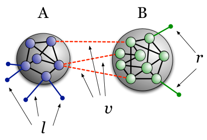
We indicate with $A$ and $B$ the two subgraphs (see Fig. 1). Let $Q_{\lambda}^{A-B}$ and $Q_{\lambda}^{AUB}$ denote the value of modularity when $A$ and $B$ are kept separated and merged, respectively.

$$Q_{\lambda}^{A-B} = \Big{[}\sum_{S\neq A,B}\dots\Big{]}+\frac{k_{in}^{A}}{2M}+\frac{k_{in}^{B}}{2M}$$ (2)

$$- \lambda\Big{(}\frac{k_{in}^{A}+l+v}{2M}\Big{)}^{2}-\lambda\Big{(}\frac{k_{in}^{B}+r+v}{2M}\Big{)}^{2},$$

where $v$ denotes the number of links joining $A$ with $B$, $l$ the number of links joining $A$ with the rest of the network (excluding $B$) and $r$ is the equivalent of $l$ for $B$. For $Q_{\lambda}^{AUB}$ we have:

$$Q_{\lambda}^{AUB} = \Big{[}\sum_{S\neq A,B}\dots\Big{]}+\frac{k_{in}^{A}}{2M}+\frac{k_{in}^{B}}{2M}+\frac{2v}{2M}$$ (3)

$$- \lambda\Big{(}\frac{k_{in}^{A}+l+v+k_{in}^{B}+r+v}{2M}\Big{)}^{2}.$$

The difference $\Delta Q_{\lambda}=Q_{\lambda}^{AUB}-Q_{\lambda}^{A-B}$ reads

$$\Delta Q_{\lambda} = \frac{2v}{2M}-\lambda\frac{k_{in}^{A}k_{in}^{B}+lk_{in}^{B}+rk_{in}^{A}+lr}{2M^{2}}$$ (4)

$$- \lambda\frac{v(k_{in}^{A}+k_{in}^{B}+l+r)+v^{2}}{2M^{2}}.$$

To simplify a little Eq. (4) we can define $\Delta=2M\Delta Q_{\lambda}$

$$\Delta = 2v-\lambda\frac{k_{in}^{A}k_{in}^{B}+lk_{in}^{B}+rk_{in}^{A}+lr}{M}$$ (5)

$$- \lambda\frac{v(k_{in}^{A}+k_{in}^{B}+l+r)+v^{2}}{M}.$$

Modularity is higher for $A$ and $B$ merged if and only if $\Delta>0$.

Eq. (5) is rather general but we are just interested in testing modularity for some special cases, for which calculations are easy. Here in particular, we will consider the case $l=r=\eta$ and $k_{in}^{A}=k_{in}^{B}=\xi$. Eq. (5) becomes

$$\Delta=2v-\lambda\frac{(\xi+v+\eta)^{2}}{M}.$$ (6)

These results are essential to follow the discussion of the next subsections.

II.2 Splitting clusters

Despite the different approaches to the problem of detecting clusters in networks, there are some general ideas which are shared by most scholars. One of them is that a random graph has no communities, so it should not be split by an algorithm in smaller pieces, with the only exception of the trivial split in singletons, i.e. in groups containing each just a single vertex, which is still an acceptable answer. Another shared belief is that a complete graph (or clique), i.e. a graph whose vertices are all connected to each other, is a perfect community (due to the fact that the internal link density reaches the highest possible value of $1$). So, if cliques are just loosely connected to each other, one would expect that a good method should detect them as separate clusters. We would like to find the mathematical conditions, in particular the choice of the resolution parameter $\lambda$, that satisfy both requisites. In this subsection we search for the condition to avoid the splitting of random subgraphs, while the condition to avoid the merger of cliques will be given in the next subsection.

Let us consider a random subgraph $\mathcal{S}$ with total degree $2M_{\mathcal{S}}$, which is part of a larger network with total degree $2M$. The goal is to check under which condition $\mathcal{S}$ is split by optimizing modularity. Here for simplicity we consider only bi-partitions. The expected optimal modularity $Q_{2}$ for the bipartition of a random graph has been computed by Reichardt and Bornholdt Reichardt and Bornholdt (2007)

$$Q_{RB}=0.765\frac{\langle\sqrt{k}\rangle_{\mathcal{S}}}{\langle k\rangle_{\mathcal{S}}},$$ (7)

where the brackets indicate expectation values over the ensemble of random graphs with the same expected degree sequence of the subgraph at study.

We now express $Q_{2}$ in terms of the number of edges $v$ between the clusters of the bipartition with optimal modularity. We obtain

$$2M_{\mathcal{S}}Q_{2}=2M_{\mathcal{S}}-2v-\frac{k_{A}^{2}+k_{B}^{2}}{2M_{\mathcal{S}}}=\frac{2k_{A}k_{B}}{2M_{\mathcal{S}}}-2v,$$ (8)

where $k_{A}$ ($k_{B}$) is the total degree of module $A$ ($B$). Since modularity is optimal when the two modules are of about equal size, i.e. when $k_{A}\approx k_{B}\approx M_{\mathcal{S}}$, we have:

$$2M_{\mathcal{S}}Q_{2}=M_{\mathcal{S}}-2v,$$ (9)

from which we can derive $v$,

$$v=M_{\mathcal{S}}\Big{(}\frac{1}{2}-Q_{2}\Big{)}.$$ (10)

Figure 2: (Color online) The plot shows $\alpha_{\mathcal{S}}$ measured on Erdös-Rényi and scale free graphs. For each type of graph we plot the analytical estimate of Reichardt and Bornholdt (RB) and a numerical estimate obtained by optimizing modularity with simulated annealing (SA) Guimerà et al. (2004). The minimum cut $v=\alpha_{\mathcal{S}}\times M_{\mathcal{S}}$ was measured by optimizing modularity for different values of $\lambda$ over the set of bipartitions. To optimize modularity, we are looking for small values of $v$ and equal values of $k^{A}$ and $k^{B}$, so tuning $\lambda$ just controls the importance of either requirement. However, simulations show that the dependence on $\lambda$ is quite weak, validating our approximation $k^{A}\approx k^{B}$.

For $Q_{2}=0$ we would have $v=M_{\mathcal{S}}/2$, which is the expected average number of links joining two modules of equal size, arbitrarily chosen. Eq. (10) implies that optimizing modularity decreases the number of expected links between the modules, with respect to arbitrary bipartitions, while it increases the internal density of links of the modules. One also sees that, for $v$ to be positive, $Q_{2}\leq 0.5$. Actually, in the calculation of Reichardt and Bornholdt, this holds only if $\langle k\rangle$ is big enough. To give an idea of the numbers that one could have, $Q_{2}\approx 0.17$ when all vertices have degree $k=20$, so $v\approx 0.33\times M_{\mathcal{S}}$ which is actually a not too bad approximation also for other degree distributions (for all vertices having degree $k=10$, $v\approx 0.25\times M_{\mathcal{S}}$). Let us call $\alpha_{\mathcal{S}}$ this proportionality factor between $v$ and $M_{\mathcal{S}}$,

$$v=\alpha_{\mathcal{S}}M_{\mathcal{S}}\;\;\textrm{and}\;\;\;k_{in}^{A}=k_{in}^{B}=(1-\alpha_{\mathcal{S}})M_{\mathcal{S}}.$$ (11)

From Eqs. (7), (10) and (11) we get

$$\alpha_{\mathcal{S}}=\frac{1}{2}-0.765\frac{\langle\sqrt{k}\rangle_{\mathcal{S}}}{\langle k\rangle_{\mathcal{S}}}.$$ (12)

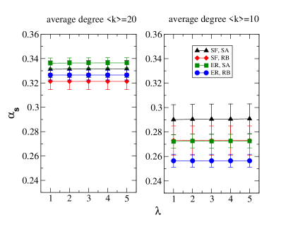
In Fig. 2 we compare the values of $\alpha_{\mathcal{S}}$ from Eq. (12) with numerical estimates derived by putting in Eq. (10) the maximum modularity $Q_{2}$, derived with simulated annealing. The calculation of $Q_{2}$ is carried out for different values of $\lambda$, but the results seem to be essentially independent of $\lambda$. We consider both Erdös-Rényi (ER) and scale-free (SF) graphs, with $1000$ vertices and average degree $\langle k\rangle=20$ (left panel) and $10$ (right panel). The SF graphs have degree exponent $2$. As we can see from Fig. 2, the analytical estimate of Eq. (12) yields a good approximation of $\alpha_{\mathcal{S}}$.

Let us now consider our splitting-merging problem, considering $A$ and $B$ as candidates. We set $\eta=1$, which means that only two links come out of $\mathcal{S}$ (ideally one from $A$, the other from $B$). In this case, we would like to have $\Delta>0$, to avoid the split of the random subgraph $\mathcal{S}$. From Eq. (6) and Eqs. (11) we get (remember that $\xi=k_{in}^{A}=k_{in}^{B}$):

$$2\alpha_{\mathcal{S}}M_{\mathcal{S}}>\frac{\lambda(M_{\mathcal{S}}+1)^{2}}{M},$$ (13)

which implies

$$\lambda<\frac{2\alpha_{\mathcal{S}}M}{M_{\mathcal{S}}}.$$ (14)

Alternatively, we can incorporate the correction factor $[M_{\mathcal{S}}/(M_{\mathcal{S}}+1)]^{2}\approx 1$ in $\alpha_{\mathcal{S}}$, so that we call $\alpha_{\mathcal{S}}$ what is actually $\alpha_{\mathcal{S}}[M_{\mathcal{S}}/(M_{\mathcal{S}}+1)]^{2}$. If the subgraph is a clique, $\alpha_{\mathcal{S}}\approx 0.5$, and modularity can even split a clique when

$$\lambda\gtrsim\frac{M}{M_{\mathcal{S}}}.$$ (15)

II.3 Merging clusters

Let us now consider two equal sized subgraphs connected with one edge ($v=1$ and $\eta=1$) and let $k_{in}^{A}=k_{in}^{B}=\xi_{\mathcal{C}}$. Eq. (6) becomes:

$$\Delta=2-\lambda\frac{(\xi_{\mathcal{C}}+2)^{2}}{M}.$$ (16)

In this case we want $\Delta<0$ (we wish to keep the two subgraphs separated), which implies

$$\lambda>\lambda_{\mathcal{C}}=\frac{2M}{(\xi_{\mathcal{C}}+2)^{2}}.$$ (17)

If $\xi_{\mathcal{C}}$ is very small, $\lambda$ has to be very big (for $\lambda_{\mathcal{C}}>1$ the subgraphs cannot be resolved by standard modularity, which corresponds to $\lambda=1$, and we recover the resolution limit of Ref. Fortunato and Barthélemy (2007)). On the other hand if $\xi_{\mathcal{C}}$ is large, the subgraphs will be resolved for a large range of $\lambda$-values.

If the subgraphs are two cliques of $n_{\mathcal{C}}$ nodes each, for instance, $\xi_{\mathcal{C}}=n_{\mathcal{C}}(n_{\mathcal{C}}-1)$.

II.4 Condition on the ineliminability of the bias

We now put together conditions (14) and (17). We have that

$$\lambda_{2}<\lambda<\lambda_{1},$$ (18)

where

$$\lambda_{1}=\frac{2\alpha_{\mathcal{S}}M}{M_{\mathcal{S}}}\;\;\textrm{and}\;\;\lambda_{2}=\frac{2M}{(\xi_{\mathcal{C}}+2)^{2}}.$$ (19)

Above $\lambda_{1}$, modularity splits random subgraphs, below $\lambda_{2}$ it puts together subgraphs even if they are connected by just one link (even in the case in which they are cliques). In the range between $\lambda_{1}$ and $\lambda_{2}$ it should be possible to avoid both biases. However, if

$$\lambda_{1}<\lambda_{2},$$ (20)

the biases cannot be both simultaneously lifted. Eq. (20) holds when, by setting $M_{\mathcal{S}}/\alpha_{\mathcal{S}}=\beta_{\mathcal{S}}$,

$${(\xi_{\mathcal{C}}+2)^{2}}<\beta_{\mathcal{S}}.$$ (21)

Note that Eq. (21) does not depend on the size of the whole network, either in terms of vertices or edges.

To be more concrete we consider a simple example. We examine a network made out of two identical cliques of $n_{\mathcal{C}}$ vertices each and an internally random subgraph of $n_{\mathcal{S}}$ vertices and average degree $\langle k\rangle_{\mathcal{S}}$. The three clusters are all connected to each other by one edge only (see Fig. 3).

Figure 3: (Color online) Schematic network with two cliques and a random subgraph, which are the natural communities of the network.

Figure 4: (Color online) This plot shows Eq. (21) as a function of $n_{\mathcal{S}}$ and $n_{\mathcal{C}}$ for the simple network with three clusters of Fig. 3 Above the curves modularity cannot find the right partition for any value of $\lambda$.

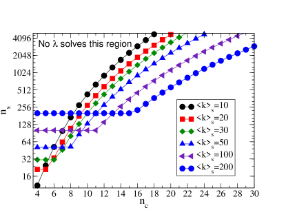
In Fig. 4 we plot the relation between $n_{\mathcal{C}}$ and $n_{\mathcal{S}}$ coming from the equality $\lambda_{1}=\lambda_{2}$ (obtained turning the inequality of Eq. (21) to an equality) for some values of $\langle k\rangle_{\mathcal{S}}$. We used Eq. (12) to evaluate $\alpha_{\mathcal{S}}$, with the approximation $\langle\sqrt{k}\rangle_{\mathcal{S}}=\sqrt{\langle k\rangle_{\mathcal{S}}}$ and the relations $\xi_{\mathcal{C}}=n_{\mathcal{C}}(n_{\mathcal{C}}-1)$ and $M_{\mathcal{S}}=n_{\mathcal{S}}\langle k\rangle_{\mathcal{S}}/2$. For any given value of $\langle k\rangle_{\mathcal{S}}$, the inequality of Eq. (21) holds above the corresponding curve.

In Fig. 5 we plot $\lambda_{1}$ and $\lambda_{2}$ as a function of $n_{\mathcal{S}}$, for $n_{\mathcal{C}}=13$ and $\langle k\rangle_{\mathcal{S}}=100$. For $\lambda_{1}$ we show two curves, one corresponding to the exact function, determined numerically, while for the other we have used the theoretical approximation of $\alpha_{\mathcal{S}}$ described above. The lines divide the $\lambda-n_{\mathcal{S}}$ plane in four areas, characterized by the presence or absence of the two biases. As we can see, the portion of the plane in which both biases are simultaneously absent (gray area) is quite small.

One might still wonder that it could be possible to find a value of $\lambda$ high enough that the random subgraph $\mathcal{S}$ is split in $n_{\mathcal{S}}$ vertices and the two cliques are still correctly detected. Let us consider Eq. $5$ when $A$ consists of a single vertex, so that $v$ is the internal degree of the vertex with respect to $B$ and $l+v=k^{A}$ is the total degree of $A$. Recalling that $k_{in}^{B}+r+v=k_{tot}^{B}$, Eq. $5$ becomes:

$$\Delta=2v-\lambda\frac{k_{tot}^{B}k^{A}}{M}.$$ (22)

Therefore $A$ and $B$ would be kept separated when:

$$\lambda>\frac{2Mv}{k_{tot}^{B}k^{A}}.$$ (23)

By increasing $\lambda$ we can actually separate some vertices of $\mathcal{S}$ and we would eventually split it in $n_{\mathcal{S}}$ clusters when $\lambda>\frac{2M}{x}$, where $x$ is the minimum $k_{i}k_{j}$ over all the connected vertices $(i,j)$ of $\mathcal{S}$. Similarly, the condition for the cliques not to be split reads:

$$\lambda<\frac{2M}{(n_{\mathcal{C}}-1)(n_{\mathcal{C}}-2)},$$ (24)

since the denominator is the total degree of a clique of $n_{\mathcal{C}}-1$ vertices (we neglected $r$) and we considered $k^{A}=v$ (the vertex does not have external connections).

In conclusion, if there are two connected vertices in $\mathcal{S}$ such that the product of their degrees is smaller than $(n_{\mathcal{C}}-1)(n_{\mathcal{C}}-2)$, no values of $\lambda$ are suitable to guess the right answer(s). This is very likely to happen if the degree distribution of $\mathcal{S}$ is broad, so that there are many low-degree vertices.

Figure 5: (Color online) Threshold parameters $\lambda_{1}$ and $\lambda_{2}$ as a function of $n_{\mathcal{S}}$ ($n_{\mathcal{C}}=13$, $\langle k\rangle_{\mathcal{S}}=100$). The theoretical line for $\lambda_{1}$ is obtained by approximating $\alpha_{\mathcal{S}}$ as described in the text. We see that $\lambda_{1}>\lambda_{2}$, up to $n_{\mathcal{S}}\approx 230$, so that no $\lambda$ can eliminate the biases for bigger values of $n_{\mathcal{S}}$. When $n_{\mathcal{S}}<\approx 230$, the biases can be both eliminated only in the shadowed area between the curves.

III Tests on benchmark graphs

We want now to check the practical consequences of the limits of multiresolution modularity. For that we take the LFR benchmark, a model of graphs with built-in community structure that we have recently introduced Lancichinetti et al. (2008). It is an extension of the planted $\ell$-partition model introduced by Condon and Karp Condon and Karp (2001). Each graph has power law distributions of degree and community size, which are common features of real graphs with community structure. The degree of mixture between clusters is measured by the mixing parameter $\mu$, expressing the ratio between the number of neighbors of a vertex outside its community and the total number of neighbors. So $\mu=0$ indicates that clusters are topologically disconnected from each other, as each vertex has neighbors within its community only, while $\mu=1$ indicates that vertices are connected only to vertices outside their group, so the groups are not communities. Vertices are linked to each other at random, compatible with the constraints on the distributions of degree and community size and to the fact that $\mu$ has to be (approximately) the same for all vertices. So the clusters are essentially random subgraphs.

We want to specialize Eq. (5) to the LFR benchmark graphs. Let us consider a cluster $\mathcal{S}$ with $n_{b}$ nodes, total degree $2m_{b}$ and internal degree $2M_{\mathcal{S}b}$. We split it into two equal-sized subgraphs such that the internal degree of either part is the same: $k_{in}^{A}=k_{in}^{B}$. Moreover, for simplicity we assume that the split is done such to keep an equal number of edges between each of the subgraphs and the rest of the network: $l=r$. We have $M_{\mathcal{S}b}=(1-\mu)m_{b}$, $l=r=\mu m_{b}$, $v=\alpha_{\mathcal{S}b}M_{\mathcal{S}b}=\alpha_{\mathcal{S}b}(1-\mu)m_{b}$. The condition of non-splitting is:

$$2v>\lambda\frac{(M_{\mathcal{S}b}+l)^{2}}{M},$$ (25)

which is:

$$2\alpha_{\mathcal{S}b}(1-\mu)m_{b}>\lambda\frac{m_{b}^{2}}{M}.$$ (26)

So,

$$\lambda<\lambda_{1}\;\;\;\textrm{where}\;\;\;\lambda_{1}=2\alpha_{\mathcal{S}b}(1-\mu)\frac{M}{m_{b}}.$$ (27)

We now search for the condition that leads to the merger of two clusters of an LFR benchmark graph. For that we should know how many edges they share, which depends on the graph size and the number of clusters. We call $v_{xy}$ the number of edges between modules $x$ and $y$ and $2m_{x}$ and $2m_{y}$ their total degrees. Eq. (5) becomes

$$\Delta=2v_{xy}-\lambda\frac{4m_{x}m_{y}}{M}.$$ (28)

The condition to keep the clusters separated is $\lambda>\lambda_{2}$, where

$$\lambda_{2}=\frac{Mv_{xy}}{2m_{x}m_{y}}.$$ (29)

So, the two biases can be simultaneously removed iff $\lambda_{1}>\lambda_{2}$, which amounts to

$$2\alpha_{\mathcal{S}b}(1-\mu)\frac{M}{m_{b}}>\frac{Mv_{xy}}{2m_{x}m_{y}}.$$ (30)

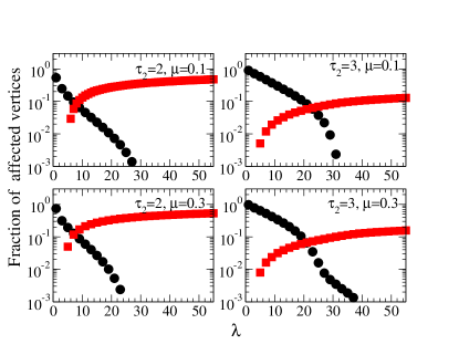
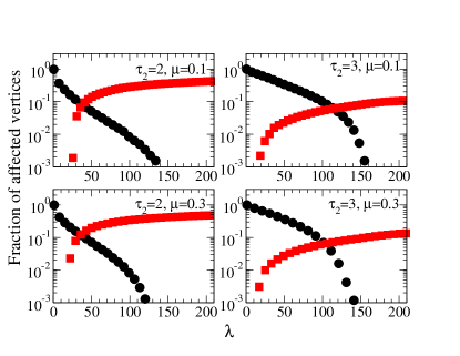
The inequality of Eq. (30) has to hold for all triples of clusters $x$, $y$ and $b$, and this is usually unlikely to happen. In order to show that, we check whether multiresolution modularity is able to deliver the planted partition of the LFR benchmark graphs for any value of the resolution parameter $\lambda$. The results are shown in Figs. 6 and 7. We plot the fraction of vertices which are incorrectly classified by modularity as a function of $\lambda$. We just consider misclassifications caused by merging (circles) or splitting (squares) the clusters of the planted partition of the graphs. We see that, for small values of $\lambda$, modularity merges many clusters and essentially splits none, whereas for large $\lambda$ there is a dominance of splitting over merging. The plots clearly show that, for every value of $\lambda$, there will be some misclassification due to cluster merging, splitting or both. The fraction of affected vertices does not go below $10\%$ but it can be considerably larger. Fig. 6 refers to graphs with $10000$ vertices, but the situation does not improve if we go to larger graph sizes ($50000$ vertices for the benchmark graphs used for Fig. 7). We point out that we have chosen low values of the mixing parameter $\mu$ ($0.1$ and $0.3$), corresponding to clusters which are well separated from each other. Modern algorithms for community detection (like Infomap Rosvall and Bergstrom (2008) and OSLOM Lancichinetti et al. (2011)) would easily find the correct partitions in the graphs we have used for the tests of Figs. 6 and 7 (see Ref. Lancichinetti and Fortunato (2009)). One may object that our estimate of the modularity maximum for each graph is just an approximation of the actual result, whose search is an NP-complete problem Brandes et al. (2006). However, we have checked in each case that the partitions found have a higher modularity than the planted partition of the benchmark graphs.

Figure 6: (Color online) Test of multiresolution modularity on LFR benchmark graphs. Each panel shows the fraction of misclassified vertices due to artificial mergers (circles) and splits (squares) of clusters, as a function of the resolution parameter $\lambda$. The panels correspond to different choices of the exponent $\tau_{2}$ of the cluster size distribution of the graph and of the mixing parameter $\mu$. Each point represents an average over $100$ benchmark graphs. All graphs have $10000$ vertices. The other parameters are: average degree $\langle k\rangle=20$; maximum degree $k_{max}=100$; minimum cluster size $c_{min}=10$; maximum cluster size $c_{max}=1000$; degree exponent $\tau_{1}=2$.

Figure 7: (Color online) Same as Fig. 6, but for LFR benchmark graphs of $50000$ vertices. All other parameters are the same as for the graphs used in Fig. 6.

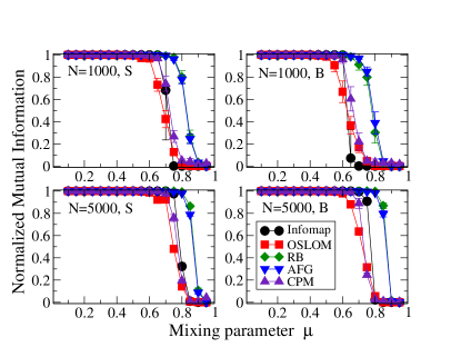
Finally we would like to check how general our results are. We have focused on the multiresolution modularity proposed by Reichardt and Bornholdt in Ref. Reichardt and Bornholdt (2006b). In this paper, however, the authors had proposed a general ansatz for the quality function, and their multiresolution modularity was just a specific case of it. In a recent work Traag et al. (2011), Traag et al. have shown that this ansatz can be specialized to include other known measures, like the multiresolution modularity by Arenas et al. Arenas et al. (2008), and the quality function adopted by Ronhovde and Nussinov Ronhovde and Nussinov (2010), which is characterized by not having a null model term, in contrast to modularity. In fact, Traag et al. derived another model from the general class of functions of Reichardt and Bornholdt, which they called Constant Potts Model (CPM), which allegedly has no resolution limit. In Fig. 8 we reproduce the results of the comparative analysis performed by Traag et al. on the LFR benchmark. Here we compare five methods: Infomap, OSLOM, the optimization of the multiresolution modularities of Reichardt and Bornholdt (RB) and Arenas et al. (AFG), and the CPM by Traag et al.. For each selected value of the mixing parameter $\mu$ we generated $100$ realizations of the LFR benchmark, and averaged on them the values of the similarity between the detected and the planted partition. As similarity measure we took the Normalized Mutual Information (NMI) Danon et al. (2005), which has become a standard in this kind of evaluations. In our computations we used a modified version of the measure lancichinetti09 , recently introduced by the authors of this paper, that is able to estimate the similarity of partitions as well as the similarity of covers, i.e., of divisions of a network into overlapping communities. We have used this version of the NMI in our comparative analysis of community detection algorithms Lancichinetti and Fortunato (2009), so we stick to it for consistency. We stress however that the clusters of the graphs we considered are not overlapping.

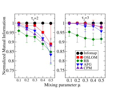
As found in Ref. Traag et al. (2011), it is possible to find values of the resolution parameter for RB and CPM, that make these methods outperform both Infomap and OSLOM. This holds for AFG as well, whose performance is essentially identical as RB. However, this is due to the fact that the cluster sizes are too close to each other, spanning less than one order of magnitude. This is demonstrated by Fig. 9, in which we take LFR benchmark graphs with the same parameters as those used for Fig. 6. Now we have $10000$ vertices and cluster sizes vary from $10$ to $1000$ vertices. Again, for the multiresolution methods we use the values of the resolution parameters that give the best results. The figure shows that the multiresolution methods fail to detect the planted partition even for very low values of the mixing parameter $\mu$, especially when the cluster size distribution is broader ($\tau_{2}=-2$). This is consistent with the results of Figs. 6 and 7. Infomap and OSLOM, on the other hand, have a clearly better performance, despite the fact that they do not have a tunable resolution parameter. In particular, Infomap always detects the right partition, for the range of $\mu$ explored here. Most networks of current interest have many more than $10000$ vertices, and accordingly community sizes span much broader ranges of values. Fig. 9 suggests that in such cases the performance of multiresolution methods might become far worse.

Figure 8: (Color online) Comparative analysis of several multiresolution techniques on the LFR benchmark. The graphs are made of $1000$ and $5000$ vertices, the exponent of the degree distribution $\tau_{1}=2$, the exponent of the clusters size distribution $\tau_{2}=1$, the average degree $\langle k\rangle=20$, the maximum degree $k_{max}=50$, the cluster size ranges are $S=[10,50]$ and $B=[20:100]$.

Figure 9: (Color online) Comparative analysis of several multiresolution techniques on the LFR benchmark. The network parameters are now the same as for the graphs used in Fig. 6. In particular, the network size is $10000$ and the cluster size spans two orders of magnitude. The two panels correspond to $\tau_{2}=2$ (left) and $\tau_{2}=3$ (right).

IV Conclusions

We have shown that multiresolution modularity maximization is characterized by two concurrent biases: the tendency to merge small clusters and to split large ones. We have seen that it is usually very difficult, and often impossible, to tune the resolution such to avoid both biases simultaneously. Tests on artificial benchmark graphs with community structure indeed show that a considerable fraction of vertices is misclassified, for any value of the resolution parameter, even when clusters are well separated and easily identified by other methods. Since, in practical applications, one knows very little about the community structure of the graphs at study, it is impossible a priori to quantify the systematic error induced by the use of modularity. Moreover, it is not easy to implement a way to “heal” the partition delivered by modularity, just because there are two sources of errors. If modularity simply combined smaller clusters in larger ones, as people have been thinking until now, one could hope to recover the real partition by looking inside the clusters delivered by modularity. Instead, since clusters can be both split and merged, the real partition must be recovered by splitting some clusters and merging others, and it is very difficult to understand which clusters contain smaller ones and which others are parts of larger clusters instead. This would require a careful exploration of groups of clusters.

Our results hold for various types of quality functions, including the recently introduced Constant Potts Model by Traag et al. Traag et al. (2011). One could argue that, after all, multiresolution methods have a remarkable performance in some cases (see Fig. 8) and a poor one in others (see Fig. 9), just like any method, including Infomap and OSLOM (from the same figures). This objection is however not sustainable, since we believe that, when clusters are so weakly connected to each other that one could even distinguish them by visual inspection, a good method cannot fail to detect them. While this is a shared view among scholars, it is still unclear where to set the limit of fuzziness between subgraphs that separates a regime in which they are clusters from one in which they are not. This problem has attracted some attention lately Bianconi et al. (2009); Lancichinetti et al. (2010). So, in the tests we reported (Figs. 8 and 9) it is not clear up to which value of the mixing parameter $\mu$ the subgraphs of the benchmark graphs are still “significant” clusters, beyond random fluctuations. But there is no doubt that they are cluster for very small values of the mixing parameter $\mu$.

We want to stress here that we are not advocating the superiority of some methods over others. The problems that we point out in this paper are probably common to many other methods. Infomap itself, for instance, is a method based on the optimization of a global measure, like modularity, and is likely to have a resolution limit as well, although it probably emerges only on large networks. In addition, it may also break random subgraphs, although its performance is perfect for well separated communities in all tests we have performed. OSLOM could be also improved, since it occasionally fails to detect the right partition for small $\mu$. Still, at variance with multiresolution methods, neither Infomap nor OSLOM have a tunable resolution parameter, so their performance is quite remarkable.

We conjecture that the tendency to simultaneously merge and split clusters is an inevitable feature of methods based on global optimization, and that it could be more easily circumvented by local approaches. Global optimization techniques work well when clusters are approximately of the same size; if clusters span a broad range of sizes, which is likely to happen on very large networks, such techniques get confused and may fail to detect some of the clusters, even when they are clearly identifiable. Resolution parameters improve things, but they do not (cannot?) solve the problem.

We hope that the scientific community working on the problem of community detection will address this issue in the future, and that general structural limits of classes of methods will be identified and, possibly, removed. In this way it will be possible to define safe guidelines to design new methods that do not suffer from such problems and that therefore could be more reliable in practical applications.