Thermalization of Strongly Disordered Nonlinear Chains

Abstract

Thermalization of systems described by the discrete non-linear Schrödinger equation, in the strong disorder limit, is investigated both theoretically and numerically. We show that introducing correlations in the disorder potential, while keeping the “effective” disorder fixed (as measured by the localization properties of wavepacket dynamics), strongly facilitate the thermalization process and lead to a standard grand canonical distribution of the probability norms associated to each site.

Introduction – The discrete nonlinear Schrödinger equation (DNLSE) continues to be an active area of research. It became a paradigm in the field of nonlinear dynamical systems [1] and it occupies an important place in nonlinear optics [2] and the theory of ultra-cold atomic Bose-Einstein condensates [3]. Much of recent work is dealing with the analysis of a wavepacket spreading, i.e. only one site (or, perhaps, a compact group of a few) is excited and the time evolution of this initial excitation is followed. The focus of this activity is the interplay of non-linearity and Anderson localization induced by a random potential [4]. A different type of problem [5, 6] is when, initially, all sites are excited, so that the amount of energy endowed to the system is proportional to its (infinite, in the thermodynamic limit) volume [7]. Following the evolution of such initial preparation one can ask whether a large isolated system thermalizes. Specifically, one can consider a large but finite part of the isolated system and ask whether it approaches a grand canonical distribution with some values of the temperature $T$ and chemical potential $\mu$.

The two types of problems, i.e. ”spreading” vs ”thermalization”, are physically distinct, as emphasized in the work of Basko [5]. In the former case, the system is excited locally (a microscopic excitation), whereas in the latter the excitation is global i.e. macroscopic. In a finite size system the distinction between the two problems can become blurred, if one does not specify how the system’s energy scales with its size. It is possible, for instance, to consider the case when the energy provided to the system remains fixed and finite, while the size of the system increases [8, 9] (the problem of a wave packet spreading belongs to this category). In such a case the system, assuming it thermalizes, will reach a temperature which is inversely proportional to system’s size and, thus, approaches zero in the thermodynamic limit.

Here we consider genuine, ”thermodynamic” thermalization, when the system’s energy is proportional to its size. We concentrate on the case of strong disorder, when in the absence of the non-linearity, all modes are strongly localized. We consider both uncorrelated and correlated random potentials and show that introducing correlations in the disorder, while keeping the effective disorder fixed (as it is measured by the spreading of an initially localized wavepacket in the absence of non-linearity), strongly facilitate the thermalization process.

Model– The time-dependent DNLSE is given by

$$i\frac{d\psi_{n}}{dt}=\epsilon_{n}\psi_{n}-v(\psi_{n+1}+\psi_{n-1})+\chi|\psi_{n}|^{2}\psi_{n},$$ (1)

where $\epsilon_{n}$ is the $n$-th site energy, while the coupling constant $v$ is set below to unity. The nonlinearity strength $\chi$ and the time $t$ are measured, respectively, in units of $v$ and $v^{-1}$. The model (1) can be interpreted as a system of coupled nonlinear classical oscillators [10, 5], with each oscillator being identified with the corresponding lattice site. We use “site” and “oscillator” interchangeably, and the same goes for “site energy” and “oscillator frequency”. Below we will consider a finite lattice $1\leq n\leq N$ with periodic boundary conditions. To define the problem completely one has to specify the sequence of $\epsilon_{n}$’s as well as the initial preparation.

We will study three kinds of $\epsilon$-sequences: (A) The step-potential where the first $N/2$ sites are assigned on -site energy $\epsilon_{\rm L}=0$, while the rest $N/2$ sites are having energy $\epsilon_{\rm R}=const\neq 0$; (B) Uncorrelated random potential where the $\epsilon_{n}$’s are independent random variables chosen from a rectangular distribution of width $2W$, centered at zero; and (C) Correlated random potential where a random sequence of $\epsilon_{n}$’s, such as in (B), is created first and then it is convoluted according to: ${\tilde{\epsilon}_{n}}={1\over\sqrt{D}}\sum_{k}\epsilon_{k}\left[0.5(1+\cos[{2\pi(n-k)\over N}])\right]^{(N/l)^{2}}$ where $D=\sum_{k}\left[(1+\cos(2\pi k/N))/2\right]^{2(N/l)^{2}}$. This choice of $D$ ensures that the second moment of the correlated potential, $\langle\tilde{\epsilon}^{2}\rangle$, is equal to that of the corresponding uncorrelated one, $\langle\epsilon^{2}\rangle$. A simple calculation shows that, for $N/l\gg 1$, the correlation function $\langle\tilde{\epsilon}_{n}\tilde{\epsilon}_{n+m}\rangle=\langle\epsilon^{2}\rangle\exp(-m^{2}/\zeta^{2})$, where the correlation length is $\zeta=l\surd 2/\pi$.

The initial wavefunction amplitudes $\{\psi_{n}\}$ associated to the $n-$th site, were chosen for all cases to be a random number in the interval $\left[0.75,1.25\right]$, while the normalization ${\cal N}=\sum_{n}|\psi_{n}|^{2}=N$ was imposed. Note that this implies that, initially, the phases of all $\psi_{n}$’s are zero. In addition to the conserved norm ${\cal N}$, the total energy of the system ${\cal H}$ is also conserved by the dynamics of Eq.  (1):

$${\cal H}=\sum_{n}[\epsilon_{n}|\psi_{n}|^{2}-v(\psi_{n}^{*}\psi_{n+1}+c.c)+\frac{1}{2}\chi|\psi_{n}|^{4}],$$ (2)

where the three terms on the r.h.s correspond, respectively, to potential, kinetic and interaction energy. The conserved quantities were monitored in our simulations to insure accuracy of the $4$rth order Runge-Kutta scheme.

Theory – We will investigate the thermalization process for the system of oscillators described by Eq. (1). We assume that the coupling between oscillators is weak. For the random cases, (B,C), this is ensured by strong disorder, i.e. by the large parameter $W/v$. For the step potential there is no randomness and the effective coupling strength depends on the initial preparation. It turns out that the aforementioned preparation corresponds to a high temperature regime, in which case the effective coupling between oscillators is weak [6, 7]. Under the weak coupling condition the thermalization criterion can be applied to an individual oscillator: in equilibrium, an oscillator with eigenfrequency $\epsilon_{n}$ should obey the grand canonical distribution (GCD) for its norm $I_{n}\equiv|\psi_{n}|^{2}$, with the phase of $\psi_{n}$ being completely random [5]:

$$P_{n}(I_{n})=\frac{1}{Z_{n}}\exp[\beta(\mu-\epsilon_{n})I_{n}-\frac{1}{2}\beta\chi I_{n}^{2}].$$ (3)

Above $\beta$ is the inverse temperature, while the partition function $Z_{n}$ is given by the integral

$$Z_{n} = \int dI_{n}\exp[\beta(\mu-\epsilon_{n})I_{n}-\frac{1}{2}\beta\chi I_{n}^{2}]$$ (4)

$$= \sqrt{\frac{\pi}{2\beta\chi}}\exp(\frac{\beta E_{n}^{2}}{2\chi})erfc(\sqrt{\frac{\beta}{2\chi}}E_{n}).$$

In Eq. (4), we have introduced the notation $E_{n}\equiv\epsilon_{n}-\mu$.

Instead of reconstructing the full distribution, we will focus our investigation (except from the case (A)) at the time average of the norm and its second moment of each individual oscillator:

$$\langle I_{n}(t)\rangle\equiv{1\over t}\int_{0}^{t}I_{n}(t^{\prime})dt^{\prime};\quad\langle I_{n}^{2}(t)\rangle\equiv{1\over t}\int_{0}^{t}I_{n}^{2}(t^{\prime})dt^{\prime}$$ (5)

Their time dependence will allow us to conclude whether or not a specific oscillator has reached equilibrium. In the long time limit, these quantities should be equal to their statistical average, with respect to the GCD given by Eqs. (3,4). The latter averaging results in:

$$\langle I_{n}\rangle = \frac{1}{\beta\chi}(\frac{1}{Z_{n}}-\beta E_{n}),$$ (6a)

$$\langle I_{n}^{2}\rangle = \frac{1}{\beta\chi}(1+\frac{\beta}{\chi}E_{n}^{2}-\frac{1}{\chi Z_{n}}E_{n}).$$ (6b)

For sufficiently weak nonlinearity, when $\chi\ll\beta E_{n}^{2}$, the partition function $Z_{n}$ can be expanded, leading to:

$$\langle I_{n}\rangle=\frac{1}{\beta E_{n}}(1-2\frac{\chi}{\beta E_{n}^{2}});\quad\langle I_{n}^{2}\rangle=\frac{2}{(\beta E_{n})^{2}}(1-5\frac{\chi}{\beta E_{n}^{2}}).$$ (7)

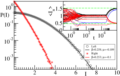
Figure 1: (Color online) Distribution $P(I)$ of the site-norm $I$ for the case of a lattice with $N=100$ sites, $\chi=1$, and a step-potential with $\epsilon_{L}=0$ and $\epsilon_{\rm R}=7.5$. Black ($\circ$)/red ($\star$) colors correspond to left/right sites. The solid lines are best fits to Eq. (3). The fitted values ($\beta_{L}=0.258;\mu_{L}=-0.109$) for the left and ($\beta_{R}=0.253;\mu_{R}=-0.1$) for the right sub-chains respectively, agree nicely (within numerical accuracy of the fit) with one-another. Inset: Evolution of the first moment of the time-averaged on-site norms $\langle I_{n}(t)\rangle$. The dashed lines are the theoretical predictions of Eq. (6a) with $\beta=0.258$ and $\mu=-0.109$. Blue lines indicate border sites $n=1$ and $n=50$.

Numerical Analysis – We now discuss our numerical results for each of the three on-site potential sequences. We start with the case (A) associated with the step potential. This is an instructive example of thermalization. We recall that the chain of $N$ sites is divided into two equal parts- the left and the right sub-chains with site energies $\epsilon_{L}=0$ and $\epsilon_{R}\neq 0$, respectively. The initial preparation with random on-site norms $I_{n}\sim 1$ evolve with time according to Eq (1). Thermalization of the system is achieved due to a significant redistribution of the norm between various sites: “flow of the norm” from the right sub-chain (large site energies) towards the left sub-chain (zero site energies) occurs during the thermalization process. At equilibrium, a strong correlation between the norm at a specific site $n$ and the potential energy $\epsilon_{n}$ is developed, so that the requirement Eq. (6) (or the more detailed condition for the full distribution) is satisfied. This scenario is confirmed by our numerical data for $\langle I_{n}\rangle(t)$, reported in the inset of Fig. 1 for a chain of $N=100$ sites with $\chi=1$ and $\epsilon_{\rm right}=7.5$. Indeed, for short times (roughly up to $t=100$) the oscillators are exchanging norm among them and the various curves fluctuate wildly and cross each other. At larger times they ”get organized” into two groups of curves (with the exception of the few border sites between the two sub-chains). Note, however, that for a long interval of time (from $t\sim 100$ till $t\sim 5\times 10^{4}$) the two groups are very close to one another and do not change with time. For still longer times, they start diverging and eventually saturate at two different values for $\langle I_{n}\rangle$ which are predicted by Eq. (6). We interpret this behavior as two-stage thermalization. First, oscillators within each sub-chain exchange norm and energy among them, with very little interaction between the two groups of oscillators. This rapid process (on time scales $t\sim 100$), leads to ”internal” thermalization, associated to each sub-chain separately. Then, at much longer times, $t\sim 5\times 10^{4}$, the slow process of interaction between the two groups of oscillators becomes efficient and it eventually leads to a full equilibrium. Thus, the potential discontinuity, between the two sub-chains, serves as a “bottleneck” which slows down the total thermalization and provides the long-time scale for the thermalization process.

We have also investigated the whole probability distribution $P(I_{n})$ for the step potential chain. After an initial transient $t\sim 10^{5}$, we have collected the norm $I_{n}$ of each oscillator at various times. In all cases more than $10^{5}$ data were used for statistical processing. We have found that the oscillators follow two distinct distributions, which are characterized by their on-site energy $\epsilon$ (i.e. left or right sub- chain) according to the prediction of Eq. (3). We have observed that the oscillators that correspond to high on-site potential energy were first to thermalize while the ones on the left sub-chain, corresponding to $\epsilon_{n}=0$, achieve thermalization with a slower rate. A representative example of $P(I_{n})$ is shown in the main panel of Fig. 1. For better statistical processing we have averaged the left and right distributions of all oscillators. We have found that both distributions $P_{\epsilon_{L}}(I)$ and $P_{\epsilon_{R}}(I)$ follow nicely Eq. (3). The corresponding fitted left and right chemical potentials and temperatures are in excellent agreement with one another, indicating that the total chain reached global thermalization.

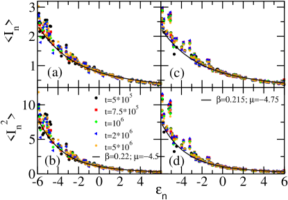
Figure 2: (Color online) First $\langle I_{n}(t)\rangle$ (a,c) and second $\langle I_{n}^{2}(t)\rangle$ (b,d) moment of the on-site norm vs. $\epsilon_{n}$ for an uncorrelated $\epsilon$-sequence with $W=6$. We considered a lattice with $N=100$ and $\chi=1$. Subfigures (a,b) and (c,d) correspond to two different initial preparations. Solid lines correspond to Eq. (6a,b)

(B) Next, we investigate the thermalization of a chain with uncorrelated on-site potential. We concentrate on the analysis of the first $\langle I_{n}\rangle$ and second moment $\langle I_{n}^{2}\rangle$ of the norm. We consider cases for which the coupling parameter, $\tau\equiv W^{-1}$ and the effective non-linearity strength $\rho\equiv\chi I_{n}/W$ are small [5]. We let the initial preparation to evolve for a long time, of the order of $5\times 10^{5}$ and then register the value of the norm $\langle I_{n}\rangle$, for all $N$ oscillators. Representative results of $\langle I_{n}\rangle$ versus the site energies $\epsilon_{n}$’s for $W=6$, $N=100$, $\chi=1$ and two different initial preparations are shown in Fig. 2a,c for times $t=5\times 10^{5};7.5\times 10^{5};10^{6};2\times 10^{6};5\times 10^{6}$. Such plot provides a check for the validity of Eq. (6) which should hold in equilibrium. In Fig. 2b,d we report also the second moment, $\langle I_{n}^{2}\rangle$. One can see that for high-energy sites $-1\leq\epsilon_{n}\leq 6$ both quantities, already for $t=5\times 10^{5}$, follow a regular curve and stay there for longer times. This part of the data is nicely fitted to the expression Eq. (6), with appropriate $\beta$ and $\mu$ values. Moreover, we have checked that for $\epsilon>4$ the norm $\langle I_{n}\rangle$ and, thus, the nonlinearity parameter become sufficiently small for the simplified relations Eq. (7) to hold. We have found, for instance, that for these highest energy tails, the relation $\langle I_{n}^{2}\rangle=2\langle I_{n}\rangle^{2}$ is satisfied quite accurately. This is an indication for a negative-exponential distribution (Eq.(3) without the nonlinear term).

We now turn to the low energy part, $\epsilon\leq-3$, of the data in Fig. 2. These sites do not show a clear sign of thermalization. The points do not fall on a regular curve but rather form a “blob”. Moreover, in the course of time the points are “jumping around” with no clear indication of approaching a regular curve. We conclude that, while the high energy sites thermalize already for relatively short times, the low energy ones do not thermalize for much longer times (of course, they well might thermalize for even longer times). Let us note that for the lowest energy sites the nonlinearity parameter $\rho$ reaches a value of about $1/2$, so that the weak nonlinearity condition [5] is not really satisfied.

(C) Finally, we discuss the case of a correlated disorder and demonstrate that the thermalization process for this case is quite different from that in (B). A random correlated sequence of $\tilde{\epsilon}_{n}$ is created as explained above (from now on we remove the “tilde”). The random correlated ensemble is characterized by the “bare” disorder $W$ and the correlation length $\zeta$. The first thing to note is that it would not be appropriate to compare uncorrelated and correlated ensembles with the same $W$; the point is that introducing correlation while keeping $W$ fixed will, generally, change the ”effective disorder” as measured, for instance, by spreading of an initially localized wave packet. Therefore the statement correlations in the randomness facilitate thermalization becomes meaningful only when the same effective disorder is kept for the cases (B) and (C). As a measure of effective disorder we chose the spreading of a particle (for $\chi=0$), initially placed at some site. More precisely, we consider the ensemble averaged $\langle\log|\psi_{n}|^{2}\rangle$, in the long time limit, where $n$ is the distance from the initial site. This quantity is plotted in Fig. 3e for two different ensembles: uncorrelated disorder (case (B)) with $W=6$ and correlated disorder (case (C) with $W=7$ and $\zeta=2.7$). Comparing the two curves one can conclude that, indeed, these two ensembles have the same effective disorder.

We are now in the position to study thermalization in a chain with correlated disorder and to meaningfully compare the results with those in Fig. 2 for the uncorrelated case. In Fig. 3a,b we report our numerical results for the correlated disorder, in the same fashion and for the same successive times as in Fig. 2. Unlike Fig. 2, now all the data, including the low energy sites, fall on one smooth curve, given by Eq. (6) with $\beta=0.11$ and $\mu=-10$. Note that the spread in the site energies here is significantly larger than in Fig. 2. This happens because in the convolution process $\epsilon_{n}$’s larger (in absolute value) than the maximal ”bare” value ($W=7$, in our case) emerge. This wide spread of $\epsilon_{n}$’s explains why the chemical potential is so low. Indeed, if the nonlinearity were very small, then Eqs. (7) would imply that $\mu$ must be considerably lower than the lowest site energy. Although in our case the nonlinearity is not very small, nevertheless, the large spread in the site energies pushes the chemical potential down (provided, that the system does thermalize).

In Fig. 3c,d we plot the numerical results for the same disorder realization as in Fig. 3a,b but with a different initial preparation. These data display an interesting feature: the green rombs or the blue triangles arrange themselves nicely in two distinct curves, which merge into one for larger $\epsilon$’s. This suggests that we have here two subsystems of sites which thermalized separately, with two somewhat different $\beta$ and $\mu$. And then, in the course of time, there is a slow process of equilibration between the two subsystems. It is tempting to suggest that the points which form the upper or lower curves originate from sites belonging to one or the other half-chain. We have checked and confirmed this hypothesis. The asymmetry between the two half-chains is due the fluctuations in $\epsilon$’s, as well as in the initial values of $I_{n}$’s. We have also studied some other disorder realizations from the aforementioned correlated ensemble. While the details of the time evolution depend on the realization and the initial preparation, we have observed in all examples an approach to equilibrium - in sharp contrast with the uncorrelated case.

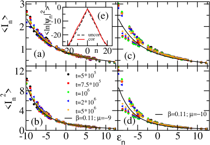
Figure 3: (Color online) Same as in Fig. 2, but for a correlated ${\tilde{\epsilon}}_{n}$-sequence with $W=7$ and correlation length $\zeta=2.7$. Subfigures (a,b) and (c,d) correspond to two different initial preparations (the same as used for Fig. 2a,b and c,d respectively). In subfigure (e) we report the asymptotic wavefunction for a linear lattice with an uncorrelated (black dashed line) and a correlated (red solid line) $\epsilon$ -sequence with $W=6$ and $W=7$ (and $\zeta=2.7$) respectively (the initial condition was a single site excitation).

Conclusions – We demonstrated that correlations in disorder strongly affects thermalization. We can offer the following intuitive explanation for this effect: In the absence of correlations (and for strong disorder) the mechanism of thermalization occurs via “resonant triples”, i.e. clusters of three oscillators with close eigenfrequencies $\epsilon_{n}$ [5]. Correlated disorder enhances the probability of occurrence of such resonant triplets, thus, facilitating thermalization. We should stress again, however, that, since in our study the strong inequalities $\tau<<1,\rho<<1$ are not satisfied, we are not quite in the regime of a very weak coupling and nonlinearity, studied in Ref. [5].

We are grateful to D. Basko for clarifications concerning Ref. [5] and to E. Gurevish, D. Shepelyansky and A. Pikovsky for useful discussions. We are particularly indebted to D. Cohen for participation in the early stage of this work and for useful advise. This research was supported by grants from AFOSR No. FA 9550-10-1-0433, the DFG Research Unit 760, and the US-Israel Binational Science Foundation (BSF), Jerusalem, Israel.

References

- [1] P. Kevrekidis, The Discrete Nonlinear Schrödinger Equation, Springer (2009); B. M. Herbst, M. J. Ablowitz, Phys. Rev. Lett. 62, 2065 (1989).
- [2] F. Lederer et al., Phys. Rep. 463, 126 (2008); D. N. Christodoulides, R. I. Joseph, Opt. Lett. 13, 794 (1988); T. Schwartz, et al., Nature 446, 52 (2007).
- [3] L. Pitaevskii and S. Stringari, Bose-Einstein Condensation, (Clarendon, Oxford, 2003).
- [4] D. L. Shepelyansky, Phys. Rev. Lett. 70, 1787 (1993); for a recent comprehensive review see J.D. Bodyfelt, et al., arXiv:1102.4604 (2011).
- [5] D. M. Basko, Ann. Phys. 326, 1577 (2011).
- [6] K. Rasmussen et al., Phys. Rev. Lett. 84, 3740 (2000); B. Rumpf, Phys. Rev. E 69, 016618 (2004); K. Rasmussen et al., Eur. Phys. J. B 15, 169 (2000).
- [7] We note that in Ref. [6], the authors investigated thermalization in clean, i.e. disordered-free, lattices.
- [8] M Mulansky et al., Phys. Rev. E 80, 056212 (2009).
- [9] D L Shepelyansky, Nonlinearity 10, 1331 (1997).
- [10] J. C. Eilbeck, P. S. Lomdahl, A. C. Scott, Physica D 16, 318 (1985); E. Wright et al., Physica D 69, 18 (1993).