I Introduction
In a probabilistic context, scale invariance is said to occur when for a set of random
variables, , with joint probability distribution , the functional form of the marginal probabilities of a -variables subset
coincides with its joint -variables probability distribution, i.e, when
|
|
|
(1) |
In the absence of independence, this relation —which is trivially fulfilled in the case of independent random variables— involves the presence of global correlations, which is precisely the scenario where nonextensive statistical mechanics Tsallis:88 ; next:04 ; next:05 ; libro ; biblio comes to play an important role.
This theory, also referred to as statistics, generalizes the standard Boltzmann-Gibbs statistical mechanics, which in turn is appropriate to describe systems which typically present local correlations, if any. In this case, the standard Central Limit Theorem (CLT) ensures the appearance of Gaussians as attractors in the thermodynamic limit for the sums of independent or weakly correlated random variables with finite variance.
Within the framework of statistics, an extension of the CLT, the so called generalized Central Limit Theorem (CLT), has been recently proved Umarov ; Umarov2 for the case of independence —a specific class of global correlations— which states that in this case the attractor distributions in the thermodynamic limit are the so called Gaussians, which in dimensions have the form Vignat ; proceedings
|
|
|
(2) |
where , is a real parameter with , is a positive constant, is a positive definite matrix, , is the so called, exponential function, whose support is for while for , and , is the normalization constant. The th order moments of distribution (2) are defined for all if , and only if for , with and a covariance matrix given by
|
|
|
(3) |
The Gaussians (as well as the independence and the standard CLT) are recovered from Eq. (2) for . Another particular instance of Gaussian is the uniform distribution, which emerges in the limit.
A number of recent works address the possible relationship between scale invariant correlations and Gaussians attractors Moyano ; Thistleton ; Hilhorst ; RodriguezSchwammleTsallis ; HanelThurnerTsallis . Though some discrete Moyano or continuous Thistleton scale-invariant systems have been shown not to have Gaussians, but remarkably close functions instead, as limiting probability distributions Hilhorst , the one-dimensional scale-invariant model introduced in RodriguezSchwammleTsallis has been analiticaly shown to yield Gaussians in the thermodynamic limit. Our goal in the present paper is to study a natural generalization of the aforementioned model to higher dimensions.
In Sec. II we go through the detailed description of scale invariance. In Sec. III we briefly review the one-dimensional model based on Leibniz-like triangles. In Sec. IV we introduce Leibniz-like pyramids and deal with the two-dimensional model. We then explore the conditional, marginal and joint probability distributions of the two-dimensional model in Sec. V. We generalize the model to arbitrary dimension in Sec. VI. Finally, we summarize our conclusions in Sec. VII. Some lengthy calculations are developed in the Appendix.
II Scale invariance
In order to illustrate the concept of scale invariance, let us consider a statistical model consisting of a set of identical and exchangeable binary random variables , taking values and . For the trivial case there are only events in the sample space and we have the probability distribution
|
|
|
(4) |
where (with , and ) stands for the probability that the variable take times the value .
For the case we have different events and the corresponding probability distribution
|
|
|
|
|
|
|
|
(5) |
where now the coefficients (with , and ) stand for the probability that the value appears times in the pair . Note that in order to have exchangeable variables the probabilities associated to events and are necessarily the same.
Let us integrate now expression (5) with respect to variable in order to obtain the corresponding marginal distribution
|
|
|
(6) |
In order to Eq. (1) be fulfilled, i.e., , it is necessary and sufficient that and .
For the case, with events in the sample space, the probability distribution reads
|
|
|
|
|
|
|
|
|
|
|
|
|
|
|
|
(7) |
where (with , and ) stands for the probability that value appears times in the event . Due to the exchangeability of variables, there are only different probabilities out of the different events. Integrating now with respect to in (7) we get the marginal distribution
|
|
|
|
|
|
|
|
|
|
|
|
|
|
|
|
(8) |
Now, for marginal distribution (8) to coincide with joint distribution (5) the relations between probabilities , and must hold.
In the general case, we have
|
|
|
(9) |
where superindex runs over the elements set of combinations of the elements set and (for ) equals if subindex is selected by combination and otherwise. The total number of summands in Eq. (9) is thus .
Integrating out with respect to in (9) one gets the marginal probability distribution
|
|
|
(10) |
which coincides with the joint probability distribution in case that
|
|
|
(11) |
This relation is known as the Leibniz rule, and reflects scale-invariance of exchangeable binary random variables. We will show a family of models satisfying relation (11) in Sec. III.
Let us consider now a set of identical exchangeable ternary variables, taking values , , and . For the case we have different events and the probability distribution
|
|
|
(12) |
where , (with ; , and )
stands for the probability of obtaining times the value and times the value .
For the case there are different events and the joint probability distribution reads
|
|
|
|
|
|
|
|
|
|
|
|
(13) |
where (with ; , and ) stands for the probability of obtaining times the value and times the value in event . Due to exchangeability, the number of different probabilities reduces to .
Integrating now with respect to one gets the marginal distribution
|
|
|
|
|
|
|
|
|
|
|
|
(14) |
which coincides with the distribution (12) when , and .
In the general case, we have
|
|
|
(15) |
where superindex runs over the elements set of combinations of the elements set , and (for ) equals if subindex belongs to the elements subset of combination , if subindex belongs to the elements subset of combination , and otherwise.
After integrating with respect to in (15) the following marginal probability distribution is obtained
|
|
|
|
|
|
|
|
(16) |
This distribution coincides with the variables joint probability distribution if
|
|
|
(17) |
We shall refer to condition (17) as the generalized Leibniz rule. We shall show a family of models satisfaying such relation in Sec. IV.
In the case of identical interchangeable ary variables taking values , the joint probability distribution reads
|
|
|
(18) |
where superindex runs over the elements set of combinations of the elements set and (for ) equals if subindex belongs to the elements subset corresponding to , for , and otherwise.
For , the joint probability distribution (18) satisfy scale invariance condition (1) if ():
|
|
|
(19) |
where , , for , and ; being a dimensional vector whose only nonzero component is the th one, taking value 1. Relation (19) reflects the scale-invariance of exchangeable nary random variables.
We shall dedicate the following sections to the detailed description of scale invariant probabilistic models.
III One-dimensional model revisited
Let us consider a random experiment which consists in flipping biased coins. We shall call the random variable that counts the number of, say, heads. can be written as
|
|
|
(20) |
where each , , is a binary random variable taking values 1 (head) with probability , and 0 (tail) with probability . As it is well known, considering that different throwings are independent of each other, we have , and the probability of obtaining heads in trials is given by
|
|
|
(21) |
with , which is no other than the binomial distribution, i.e., , with and , where the binomial coefficients stand for the different ways in which the heads can be obtained. In other words, though there are different events in the sample space, only among them are assigned different probability values, namely , , (it is irrelevant which specific coins yield head, only counts the number of them). These selected probability values may be displayed in a triangle in the form
|
|
|
|
|
|
|
|
|
|
|
|
|
|
|
|
|
|
|
|
1 |
|
|
|
|
|
|
|
|
|
|
|
|
|
|
|
|
|
|
|
|
|
|
|
|
|
|
|
|
|
|
|
|
|
|
|
|
|
|
|
|
|
|
|
|
|
|
|
|
|
|
|
|
|
|
|
|
|
where the -th row displays the probabilities, , for . In order to get the actual probabilities (21) the above triangle has to be multiplied, element by element, by the Pascal triangle.
Let us now show explicitly the scale invariant character (which otherwise follows trivially due to the independent character of the variables) of our probabilistic model. Any of the binary variables follows a Bernoulli distribution, with or 1, and . Thus, as the variables are independent, we have
|
|
|
(22) |
Considering now the marginal distribution corresponding to the first variables one gets
|
|
|
|
|
|
|
|
(23) |
|
|
|
|
so a discrete version of Eq. (1) is fulfilled and the model is scale-invariant. In addition, it is readily seen that coefficients displayed in the above triangle follow the Leibniz rule (Eq. (11), which, as stated in Sec. II, serves as an alternative description of scale invariance for binary variables). Thus, following Eq. (11), the sum of two consecutive coefficients in any row of the triangle yields the coefficient on top of them.
Let us recall that the CLT states that, after properly centering and rescaling, one obtains a Gaussian (which can be seen as a Gaussian with ) distribution out of (21), namely for . We shall try now to modify the model so as to obtain Gaussians with in the thermodynamic limit.
III.1 Scale-invariant triangles
So far, we have considered independent variables. We shall now introduce correlations in the model in such a way that the Leibniz triangle rule (11) is preserved —that is, scale invariant correlations— by substituting the probabilities in (21) by appropriate ones. In other words, we shall change the above triangle by
another one also satisfying (11). As a first attempt, we may resort to the so called Leibniz harmonic triangle Polya , whose coefficients, defined us
|
|
|
(24) |
where is the Beta function, may be displayed in triangular form us
|
|
|
|
|
|
|
|
|
|
|
|
|
|
|
|
|
|
|
|
|
|
|
|
1 |
|
|
|
|
|
|
|
|
|
|
|
|
|
|
|
|
|
|
|
|
|
|
|
|
|
|
|
|
|
|
|
|
|
|
|
|
|
|
|
|
|
|
|
|
|
|
|
|
|
|
|
|
|
|
|
|
|
|
|
|
|
|
|
|
|
|
|
|
|
|
|
|
|
|
|
|
|
|
|
|
|
|
|
|
|
|
|
|
|
|
|
|
|
|
|
|
|
|
|
|
|
|
|
Making use of the properties of the Beta function it is a simple task checking that the Leibniz triangle above satisfies the rule (11) which, for this reason, is named Leibniz rule.
Substituting now the coefficients by the Leibniz coefficients (24) in Eq. (21) we obtain
|
|
|
(25) |
with , that is, a uniform distribution, which, in the continuum limit, corresponds, as already mentioned in Sec. I, to a Gaussian with .
A family of scale-invariant triangles can be now obtained as properly normalized subtriangles of the Leibniz triangle in the following fashion. Take the central coefficient of any even row of the Leibniz triangle and divide the whole triangle by it so as to turn the said coefficient to one. Now take this coefficient as the vertex of a new triangle starting downwards from it. The coefficients of this new triangle starting from the th row of the Leibniz triangle can be then expressed as a function of the coefficients of the Leibniz triangle as
|
|
|
(26) |
As the only transformation we have made on the coefficients of the Leibniz triangle is a multiplication by a constant factor, Eq. (11) still holds for the coefficients (26), thus
|
|
|
(27) |
for any positive integer . In virtue of Eq. (27), different coefficients of the triangle are not independent of each other and it suffices to specify one element of each row (for instance the left side of the triangle) to completely determine the whole triangle.
Expressing now the Leibniz triangle coefficients in (26) in terms of the Beta function as in (24), one easily gets
|
|
|
(28) |
where now may take any positive value (see details in HanelThurnerTsallis ).
Apart from its symmetry, it is worth noticing another remarkable property of coefficientes (28), namely, scale invariance condition (27) guarantees that the set of corresponding probability distributions
|
|
|
(29) |
associated to the new set of variables
|
|
|
(30) |
are well defined, that is, the normalization condition, , holds for any value of . It may be shown that for all and . Concerning the binary variables in the sum (30) (taking values 0 and 1 as in the independent case), it may be shown that now , and for . The constant value of the correlations, which are independent of the system size and the pair of chosen variables , reveals the scale-invariant character of the model.
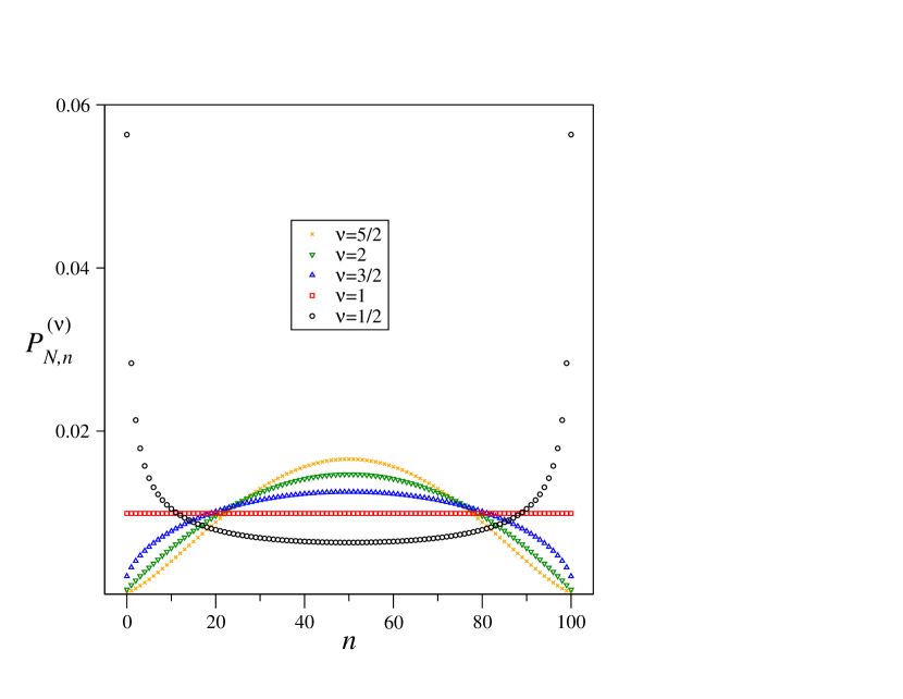
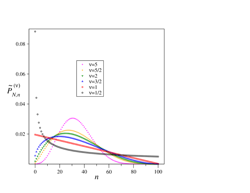
Probability distributions (29) are shown in Fig. 1 for and , 1, , 2 and .
III.2 Boltzmann and thermodynamic limits
The limits (that we shall call Boltzmann limit for a reason to be clear soon) and (thermodynamic limit) are interchangeable in (28) (equivalently in (29)). In effect, in the first case on has , so
|
|
|
(31) |
and a binomial distribution with (fair coin), associated to variable is recovered, which is consistent with the fact that , thus having independent coins. Then, as the CLT states, by properly centering and rescaling variable , one gets a Gaussian out of (31) in the thermodynamic limit.
The limit is much more subtle. It was studied in RodriguezSchwammleTsallis and later extended in HanelThurnerTsallis . Depending on the change of variable used when passing from the discrete to the continuous model, two families of Gaussians are obtained out of (29) in the thermodynamic limit, with values of given by for or for . Note that two different conjugated Gaussians exist for each HanelThurnerTsallis . In any case, one gets , so the ordinary Gaussian is recovered again.
To further support our claim, we typify variable by making the change
|
|
|
(32) |
with and compare its probability distribution with the corresponding one-dimensional Gaussian (2) with and so as to obtain unit variance
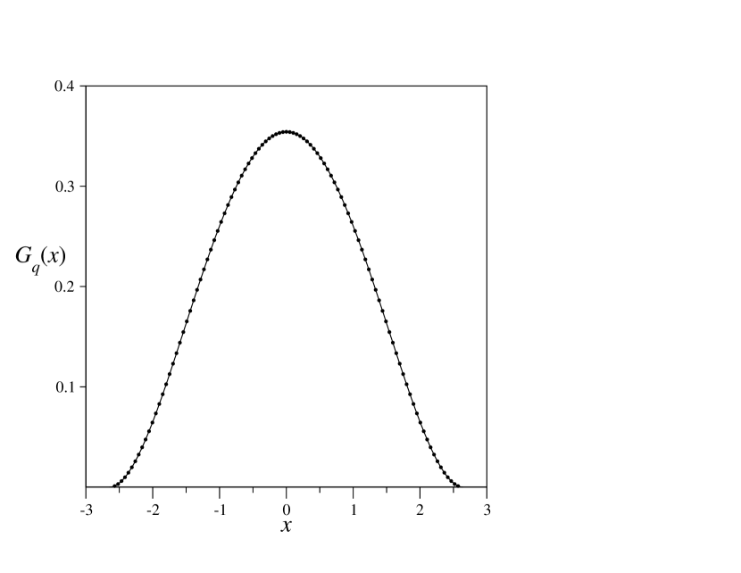
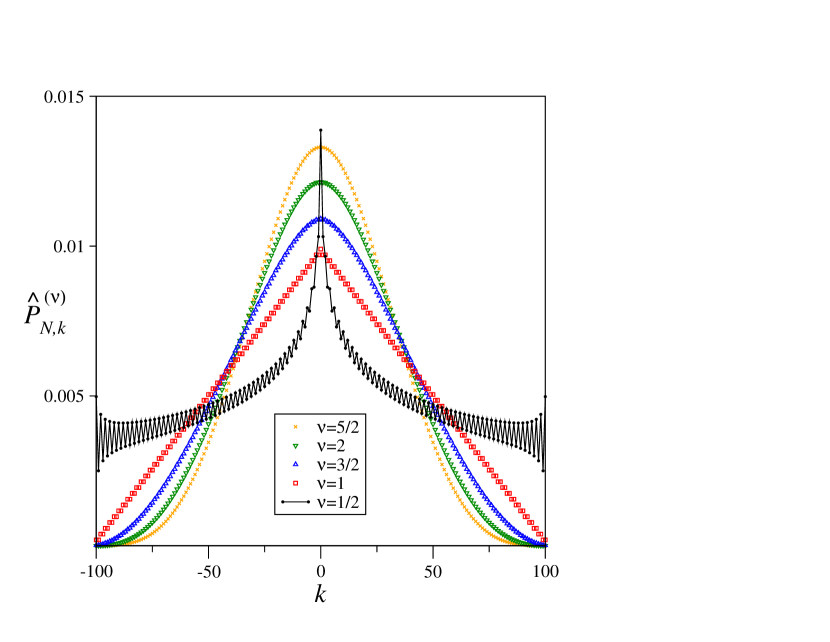
(see Eq. (3)). Fig. 2 shows
versus for and (dots) compared with the corresponding Gaussian with and unit variance (solid line). The agreement is surprisingly good, even for smaller (not shown) values of .
IV Two-dimensional model
Let us now generalize our random experiment to one with three different outcomes, which is equivalent to throw a biased three-sided dice. Let us label the sides , and and suppose that the associated probabilities are , , with , and . To properly describe our model we need to define a two components random variable
|
|
|
(33) |
with , as a sum of ternary variables , for , with values (side ), (side ) and (side ). Thus counts the number of ’s and , with , counts the number of ’s out of throwings. For independent dices the variables are independent of each other, though variables , within each pair are not (, , , , ), neither the variables and , for which , and the covariance matrix is given by
|
|
|
(34) |
The probability of having ’s and ’s, with , in throwings is given by
|
|
|
(35) |
with , which is the trinomial distribution, i.e., , where the trinomial coefficients, , take into account the degeneracy since among the different events in the sample space only of them have different probabilities, namely . These probability values may be displayed in a pyramid
where each layer, corresponding to a different value of , is a triangle
with elements, whose rows, from top to bottom, correspond to increasing values of from 0 to , while the ascending (descending) diagonals, from left to right (right to left), correspond to increasing values of () from 0 to .
In order to get the actual probabilities (35) the above pyramid has to be multiplied by the so called Pascal pyramid
|
|
|
|
|
|
|
|
|
|
|
|
|
|
|
|
|
|
|
|
|
|
|
|
|
|
|
|
|
|
|
|
|
|
|
|
|
|
|
|
1 |
|
|
|
|
|
|
|
4 |
|
4 |
|
|
|
|
|
6 |
|
12 |
|
6 |
|
|
|
4 |
|
12 |
|
12 |
|
4 |
|
| 1 |
|
4 |
|
6 |
|
4 |
|
1 |
|
|
|
|
|
|
|
|
|
|
1 |
|
|
|
|
|
|
|
|
|
5 |
|
5 |
|
|
|
|
|
|
|
10 |
|
20 |
|
10 |
|
|
|
|
|
10 |
|
30 |
|
30 |
|
10 |
|
|
|
5 |
|
20 |
|
30 |
|
20 |
|
5 |
|
| 1 |
|
5 |
|
10 |
|
10 |
|
5 |
|
1 |
|
|
|
|
|
|
|
|
|
|
|
|
|
which displays the trinomial coefficients (for the values of and within each layer the same comments as above hold).
The joint probability distribution for the independent ternary variables is now , with , and , or . In an analogous fashion as in Eq. (23), it may be shown that , so the model, as mandated by the independence of the variables, still remains scale-invariant. In turn, it is easily seen that coefficientes follow the generalized Leibniz rule (17), which, as stated in Sec. II, governs scale invariance for ternary variables.
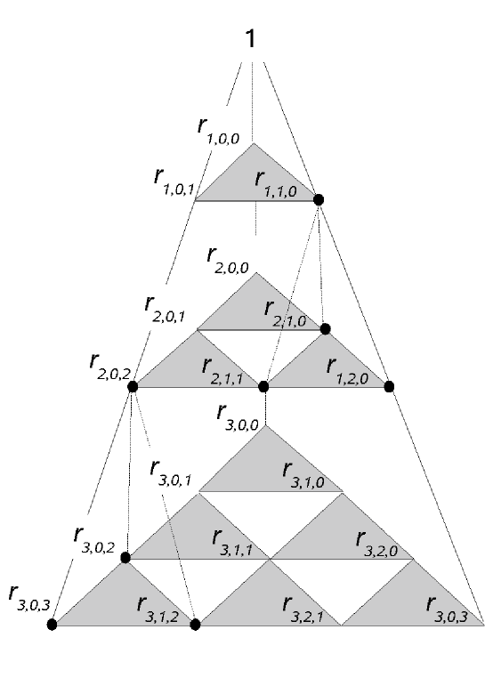
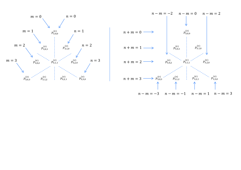
Thus, following Eq. (17), adding up three elements forming specific triangles within a layer (only those triangles formed by two consecutive elements of any row and the one on top of them),
one gets the coefficient just on top of them (belonging to the above layer). Fig. 3 shows the first four layers of the pyramid. Only the shaded triangles contribute to the generalized Leibniz rule. Two particular sets of four elements satisfying the generalized Leibniz rule are shown.
In analogy with the one-dimensional case, the corresponding bidimensional version of the CLT states that the trinomial distribution yields a bidimensional Gaussian in the thermodynamic limit, that is, for we have , with already given in (34).
Our next step is to analyze under what conditions this type of model can provide bidimensional Gaussians.
IV.1 Scale-invariant pyramids
As we did in Sec. III.1, we shall now introduce scale-invariant correlations in the model, so different dice throwings will no longer be independent. With this purpose, we may extend the Leibniz triangle to a Leibniz-like (tetrahedral) pyramid:
|
|
|
|
|
|
|
|
|
|
|
|
|
|
|
|
|
|
|
|
|
|
|
|
|
|
|
|
|
|
|
|
|
|
|
|
|
|
|
|
|
|
|
|
|
|
|
|
|
|
|
|
|
|
|
|
|
|
|
|
|
|
|
|
|
|
|
|
|
|
|
|
|
|
|
|
|
|
|
|
|
|
|
|
|
|
|
|
|
|
|
|
|
|
|
|
|
|
|
|
|
|
|
|
|
|
|
|
|
|
|
|
|
|
|
|
|
|
|
|
|
|
|
|
|
|
|
|
|
|
|
|
|
|
|
|
|
|
|
|
|
|
|
|
|
|
|
|
|
|
|
|
|
|
|
|
|
|
|
|
|
|
|
|
|
|
|
|
|
|
|
|
|
|
|
|
|
|
|
|
|
|
|
|
|
|
|
|
|
|
|
|
|
|
|
|
|
|
|
|
|
|
|
|
|
|
|
|
|
|
|
|
The coefficients are given by
|
|
|
(36) |
They satisfy the generalized Leibniz condition (17), and are defined in such a way that, when multiplying element by element by the Pascal pyramid, we get for the actual probabilities a uniform distribution:
|
|
|
(37) |
with , which again leads as to a (bidimensional) Gaussian with .
As we did with the triangles, we can now get a family of scale-invariant pyramids out of the Leibniz-like pyramid. As the only layers of the pyramid with a central coefficient are those multiple of 3, we shall descend 3 by 3 layers from the top of the Leibniz pyramid and divide the whole pyramid by the corresponding central element, that is, the element of the th layer. This coefficient so turns to unity and we can start a new pyramid downwards from it, with coefficients given by
|
|
|
(38) |
By construction, the family of pyramids (38) satisfy the generalized Leibniz rule (17) (see comment following Eq. (26)), hence
|
|
|
(39) |
for any positive integer . Due to restriction (39) on the pyramid coefficients, the whole pyramid may be determined by only specifying the elements of one face.
Expressing the trinomial coefficient in (36) as a product of binomial coefficients and making use of the property of the Beta function expressed in (24), the coefficients of the Leibniz-like pyramid can alternatively be expressed as
|
|
|
(40) |
Introducing now (40) in (38), after some algebra, one finally gets
|
|
|
(41) |
where now can take on any positive value.
Multiplying the Pascal pyramid by the family of pyramids (41), one gets a family of probability distributions
|
|
|
(42) |
with for any , associated to the new family of statistical variables
|
|
|
(43) |
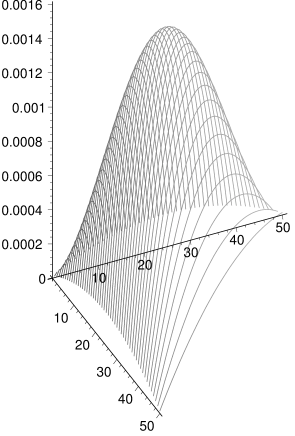
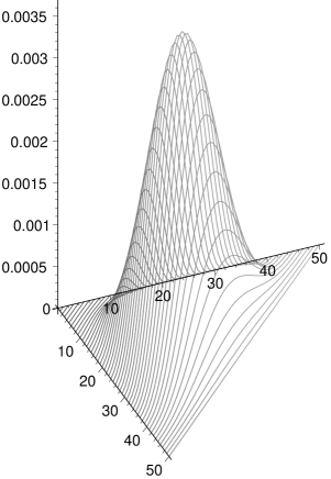
Fig. 4 shows probability distributions (42) for and , 1 (uniform distribution in the triangle ), 2 and 5.
It may be shown that and the covariance matrix is
|
|
|
(44) |
Concerning the ternary variables in the sum (43) (which take the same values as the ternary independent variables in (33)), they are no longer independent of each other, their first and second order moments being given by
, , for , and for . The scale-invariant character of the correlations that we have introduce becomes, as before, apparent.
IV.2 Boltzmann limit
Taking limits in (41) one gets , so in the Boltzmann limit the trinomial distribution
|
|
|
(45) |
with is obtained (as well as covariance matrix (44), in the Boltzmann limit, coincides with covariance matrix (34) for the same values of and ), which is again consistent with the fact that , so independent dices are recovered. Applying now the CLT, a Gaussian distribution appears again in the thermodynamic limit.
We will devote Sec. V to the study of probability distribution (42), in particular its thermodynamic limit, in order to check if it is a bidimensional Gaussian.
IV.3 Entropy
As it was shown in Ref. RodriguezSchwammleTsallis , the family of distributions (29) based on scale-invariant triangles (28), are properly described by the Boltzmann-Gibbs entropy. It has been recently shown (see HanelThurner and references therein) that this is so due to the fact the number of microstates increases exponentially with the system size (). In turn, the nonadditive entropy with Tsallis:88 (the case corresponds to the Boltzmann entropy)
turns out to be appropriate (in the sense that the entropy is extensive) to describe systems for which a relevant fraction of the degrees of freedom vanishes in the thermodynamic limit HanelThurner . Such is the case for the binary models studied in MarshFuentesMoyanoTsallis , corresponding to triangles where the nonzero probabilities restrict, in the thermodynamic limit, to a strip of size on the triangle, being well described by the nonadditive entropy with (more precisely, for this value of , is extensive).
For the ternary model (42) we also have exponential increase of the phase volume (), so, once again, the Boltzmann entropy is expected to be extensive. The nonadditive entropy for the family of pyramids (41) is given by
|
|
|
(46) |
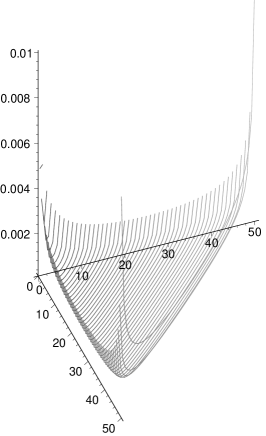
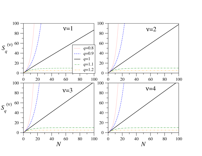
for and for . Fig. 5 shows
entropy (46) as a function of for different values of and . As predicted, independently of the value of , the value of which makes the entropy extensive is .
V Joint, conditional and marginal distributions
In order to get a deeper insight into the two-dimensional probability distribution (42) we shall start by studying its associated one-dimensional marginal distributions since, as stated in Ref. Vignat , in case these distributinos were Gaussians, the two-dimensional one would also be Gaussian, with values of related by , where () stands for the value of corresponding to the one- (two-)dimensional Gaussian.
By construction, probability distribution (42) inherits the highly symmetrical character of the trinomial coefficients (any layer of the Pascal pyramid is a triangle symmetric with respect to any of its heights) and so (the same property holds for coefficients (41)). Thus the marginal distributions , and , associated to variables , and (which, as shown in Fig. 6, correspond respectively to adding up probabilities along the ascending diagonals, descending diagonals or rows of the layers of the pyramid) are identical. Fig. 7 shows probability distributions for and , 1, , 2, and 5. The first apparent property of these distributions is its nonsymmetric character, their first moments being given by and, as easily deduced from (44), . This asymmetry vanishes when (as stated in Sec. IV.2, in the Boltzmann limit, bidimensional distribution (42) tends to a symmetric trinomial distribution, thus having symmetric binomial marginal distributions) but remains when increasing (it may be shown that the skewness coefficient assymptotically approaches a finite value in the thermodynamic limit).
A new family of nonsymmetric triangles can be defined from the marginal distributions in the form
|
|
|
(47) |
The instance of triangles (47) is
|
|
|
|
|
|
|
|
|
|
|
|
|
|
|
|
|
|
|
|
|
|
|
|
|
|
|
|
|
|
|
|
|
|
|
|
|
|
|
|
|
|
|
|
|
|
|
|
|
|
|
|
|
|
|
|
|
|
|
|
|
|
|
|
|
|
|
|
|
|
|
|
|
|
|
|
|
|
|
|
|
|
|
|
|
|
|
|
Though asymmetric, triangles (47) fulfill scale-invariance condition (27). In fact, they can alternatively be obtained applying rule (27) to the edge of the corresponding pyramid.
In addition, for integer values of , triangles (47) may be obtained as nonsymmetric, properly rescaled subtriangles of the family (28) in the form
|
|
|
(48) |
From (48), the marginal probabilities can be related to the one-dimensional family (29) in the form
|
|
|
(49) |
which, for , reduces to the straight line
|
|
|
(50) |
shown in Fig. 7.
The nonsymmetric character of marginal distributions makes them not good candiates to yield Gaussians in the thermodynamic limit. Nevertheless, there is another yet unexplored direction for the marginal distributions. We shall now add up coefficients in the vertical direction of each layer, which corresponds to calculate the marginal distribution associated to the variable (see Fig. 6). Fig. 8 shows marginal distributions for and , 1, , 2 and . Contrary to the former case, these new marginal distributions are symmetric, due to the aforementioned fact that the layers of the pyramid are symmetric triangles with respect to their heights. From these distributions and dividing by the appropiate binomial coefficient, we can now define a new family of triangles in the form
|
|
|
(51) |
with only even labelled rows. The instance of triangles (51) is
|
|
|
|
|
|
|
|
|
|
|
|
|
|
|
|
|
|
|
|
|
|
|
|
|
|
|
|
|
|
|
|
|
|
|
|
|
|
|
|
|
|
|
|
|
|
|
|
|
|
|
|
|
|
|
|
|
|
|
|
|
|
|
|
|
|
|
|
|
|
|
|
|
|
|
|
|
|
|
|
|
|
|
|
Though symmetric triangles (51) share their sides with one of the sides of triangles (47) and the edge of pyramids (41), i.e., , it should be stressed that they are not scale invariant. To properly define scale invariance in triangles (51), Leibniz rule (11) can recursively be applied to connect coefficients separated two rows, thus obtaining . This relation is not fulfilled by triangles (51). Nevertheless, it is asymptotically fulfilled in the thermodynamic limit. In effect, we shall define the quotient
|
|
|
(52) |
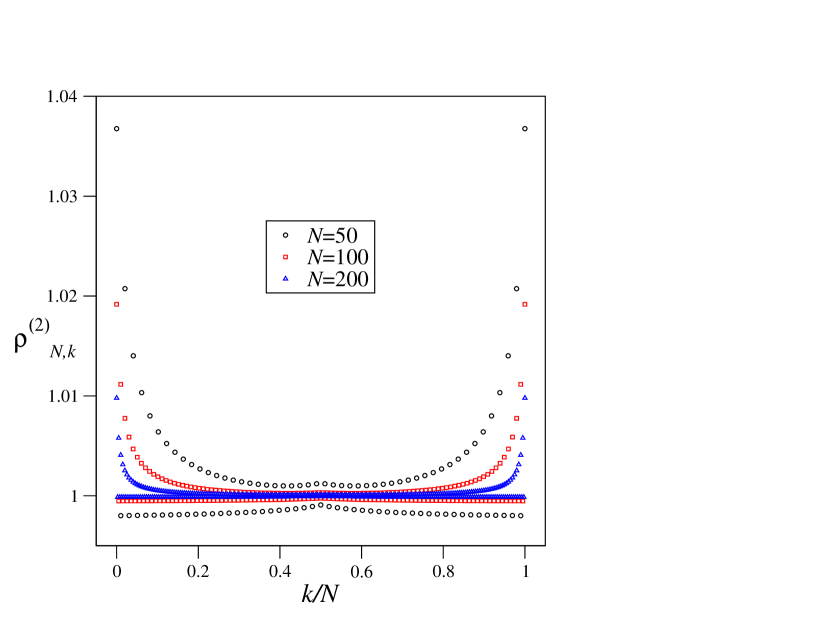
and show that . Fig. 9 shows quotient (52) versus for and , and . An oscillating trend around the value 1 is observed, the quotient being closer to 1 for the central values of . Increasing makes closer to 1. We then verify that triangles (51) are asymptotically scale invariant.
There is, however, an alternative way of obtaining the same above distributions . Let us think of our ternary variables as being scalars —instead of vectors, as imposed in (43)— having values , 0 and 1. We shall denote them by , , and consider the sum of them , which is a scalar variable having values in . If we associate the probabilities of pyramid (42) to the probability of having variables with value 1 and variables with value , the probability distribution of variable exactly coincides with the marginal distribution of distribution (42). Thus, in our model the dimension associated to the random variables plays a secondary role, the specific form of the correlations among them being of major importance. Some numerical results seem to indicate that marginal distributions do not yield Gaussians in the thermodynamic limit either. Nevertheless, the difficulty to reach high values of (due to the rapidly increasing value of the trinomial coefficients) doesn’t allow us to establish a definite conclusion.
Let us turn now to the study of the conditional distributions of probability distribution (42), which are defined in the way
|
|
|
(53) |
and an equivalent expression for , which, for symmetry considerations, is identical. We show in the Appendix that
|
|
|
(54) |
i.e., the conditional distributions of the family of distributions (42) coincide with the family (29), already shown in Fig. 1, for an appropiate system size.
Thus, bidimensional distribution (42) contains sections which, as stated in Sec. III.2, are Gaussians in the thermodynamic limit, which is a necessary, but by no means sufficient condition for probability distributions (42) to be two-dimensional Gaussians.
To further explore the nature of distribution (42) we will do the following. Let us first typify variable by making the linear change
|
|
|
(55) |
with jacobian , where matrix is defined in such a way that , with given in (44), thus
|
|
|
(56) |
Vector random variable defined in (55) is centered, i.e., , where , and has identity covariance matrix, since .
In addition, change (55) has the extra effect of converting triangle of vertices , and , into a centered in the origin and equilateral triangle of vertices , and , with , more appropiate for our purpose.
In the hypothesis that distribution (42) yields a bidimensional Gaussian with in the thermodynamic limit, we shall compare probability distribution of variable with a typified bidimensional Gaussian (2) with and (thus having identity covariance matrix as ensured by Eq. (3)).
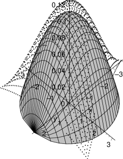
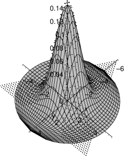
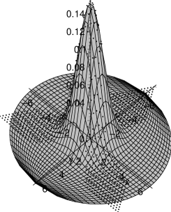
Fig. 10 plots versus (dots) compared with the corresponding bidimensional -Gaussian (solid surface), for and , (left), , (center) and , (right). For the mismatch is evident, the results not improving when increasing , neither by changing the value of . Nevertheless, when increasing the fitting improves, which is due to the fact that, as stated in Sec. IV.2, family (42) approaches a trinomial distribution in the Boltzmann limit, which in turn approaches a Gaussian distribution in the thermodynamic limit, while the corresponding Gaussian also approaches a Gaussian since .
Thus, bidimensional Gaussians with generic values of are elusive in the present model. A possible reason for it is the inadequacy of linear change (55). Instead, a nonlinear (and highly not trivial) change is needed, which transforms the triangle into a circle (either for all values of , or at least for increasing ). Research along this line is in progress.
VI Generalization of the model to arbitrary dimension
We may now throw a four-sided dice (i.e., a tetrahedric dice), with associated probabilities , , (with ), and for the different sides. We need now a three components variable
|
|
|
(57) |
with , defined as a sum of quaternary variables , for , taking the four possible values , , and associated to the different sides, so that , and count the number of appearences of three of the sides out of throwings. Variable follows the tetranomial distribution
|
|
|
(58) |
where and the tetranomial coefficients, , stand for the number of ways in which the same result can be obtained after throwings. We have now different events, though only different probability values, namely . In order to display them (what we will not do) we would need to use a elements pyramid for each value of (in the same way as we used a elements triangle for each value of for the trinomial distribution and a elements row for each value of for the binomial distribution). Putting all the pyramids together makes a hyperpyramid (in the same way as we got a pyramid made of triangles for the trinomial distribution and a triangle made of rows for the binomial distribution). In order to get the actual probabilities (58), this hyperpyramid should be multiplied by what we may call Pascal hyperpyramid
|
|
|
|
|
|
|
|
|
|
|
|
|
|
|
|
|
|
|
|
|
|
|
|
|
|
1 |
|
|
|
|
|
|
3 |
|
|
|
|
|
3 |
|
3 |
|
|
|
|
|
3 |
|
|
|
|
|
6 |
|
6 |
|
|
|
3 |
|
6 |
|
3 |
|
|
|
|
1 |
|
|
|
|
|
3 |
|
3 |
|
|
|
3 |
|
6 |
|
3 |
|
| 1 |
|
3 |
|
3 |
|
1 |
|
|
|
|
|
|
1 |
|
|
|
|
|
|
|
|
4 |
|
|
|
|
|
|
|
4 |
|
4 |
|
|
|
|
|
|
|
6 |
|
|
|
|
|
|
|
12 |
|
12 |
|
|
|
|
|
6 |
|
12 |
|
6 |
|
|
|
|
|
|
4 |
|
|
|
|
|
|
|
12 |
|
12 |
|
|
|
|
|
12 |
|
24 |
|
12 |
|
|
|
4 |
|
12 |
|
12 |
|
4 |
|
|
|
|
|
1 |
|
|
|
|
|
|
|
4 |
|
4 |
|
|
|
|
|
6 |
|
12 |
|
6 |
|
|
|
4 |
|
12 |
|
12 |
|
4 |
|
| 1 |
|
4 |
|
6 |
|
4 |
|
1 |
|
|
which displays the tetranomial coefficients. Now, layers from top to bottom within th pyramid, correspond to constant values of from 0 to . In addition, rows from bottom to top within each layer correspond to constant values of from 0 to , while indexes and behave in the same way as in the Leibniz pyramid.
We may define now the Leibniz hyperpyramid as
|
|
|
(59) |
whose coefficients may be displayed as
So defined, when multiplying Pascal hyperpyramid by Leibniz hyperpyramid one obtains the uniform tridimensional distribution given by
|
|
|
(60) |
In adittion, a family of hyperpyramids may be extracted from the Leibniz hyperpyramid (59) in the way
|
|
|
(61) |
for any positive integer , which satisfy a furtherly generalized Leibniz rule
|
|
|
(62) |
which states that adding up certain four elements subpyramids of the th pyramid (analogous to the subpyramids of the Leibniz-like pyramid depicted in Fig. 3) one gets a corresponding element of the th pyramid. Relation (62) is the instance of relation (19).
In order to get an explicit expression for coefficients (61), we shall first rewrite Leibniz-like triangle coefficients (28) in the form
|
|
|
(63) |
and correspondingly, coefficients (41) of the Leibniz-like pyramids in the form
|
|
|
(64) |
which naturally leads us to rewrite the coefficients (61) of the family of hyperpyramids as
|
|
|
(65) |
which satisfy relation (62) for any .
Generalizing former results, the corresponding family of probability distributions
|
|
|
(66) |
associated to random variable ,with for all and covariance matrix
|
|
|
(67) |
yields a tetranomial distribution, with , in the Boltzmann limit:
|
|
|
(68) |
where independent dices are recovered.
We are finally prepared to extend the above structure to higher dimensions. To describe a random experiment consisting of throwing a -sided dice times, we need a dimensional random variable
, with
|
|
|
(69) |
where , , is the -dimensional, -valued random variable associated to the th throw, taking values for side labelled 1, for side labelled 2, , for side labelled , and for side labelled ( corresponds to binary variables, corresponds to ternary variables, and so on). Thus, variable , for , counts the number of appearances of side labelled out of throwings.
Variable follows a multinomial distribution
|
|
|
(70) |
where stands for the probability of obtaining side , , and the multinomial coefficients, , stand for the different ways to obtain the result . Thus, there are only different probability values, namely among the events of the sample space.
The -dimensional Leibniz hyperpyramid is given by
|
|
|
(71) |
from which the family of hyperpyramids
|
|
|
|
|
|
|
|
(72) |
with associated probabilities
|
|
|
(73) |
for variable is obtained, with for all , and covariance matrix
|
|
|
(74) |
(concerning the component variables , . , one has , , , for , , for , and , for and .)
The generalized scale invariance rule, followed by coefficients (72) for , is given in Eq. (19).
