Orbits of the Kepler problem via polar reciprocals

Abstract

It is argued that, for motion in a central force field, polar reciprocals of trajectories are an elegant alternative to hodographs. The principal advantage of polar reciprocals is that the transformation from a trajectory to its polar reciprocal is its own inverse. The form of polar reciprocals $k_{*}$ of Kepler problem orbits is established, and then the orbits $k$ themselves are shown to be conic sections using the fact that $k$ is the polar reciprocal of $k_{*}$. A geometrical construction is presented for the orbits of the Kepler problem starting from their polar reciprocals. No obscure knowledge of conics is required to demonstrate the validity of the method. Unlike a graphical procedure suggested by Feynman (and amended by Derbes), the algorithm based on polar reciprocals works without alteration for all three kinds of trajectories in the Kepler problem (elliptical, parabolic, and hyperbolic).

Approximately, a hodograph is a plot of velocities along a trajectory; more precisely, it is the locus of the tips of the velocity vectors after they have been parallelly transported until their tails are at the origin (in velocity space). There have been many articles on the pedagogic virtues of hodographs.Abelson ; Gonzalez ; Apostolatos ; Butikov ; Mungan Feynman’s Lost LectureFLL contains, amongst other things, a recipe for drawing the elliptical path of a planet given its hodograph. The procedure, as reproduced in Ref. FLL, , has some shortcomings,Griffiths ; Weinstock but, fortunately, these have been more than satisfactorily rectified by Derbes.Derbes Derbes notes that Feynman’s scheme also works for hyperbolic orbits and he is able to devise another construction for the exceptional case of parabolic orbits. A completely different way of tracing all three kinds of orbits with the help of hodographs has been successfully developed by Salas-Brito and co-workers in a series of publications culminating in Ref. SalasBrito, .

The various geometrical methods of the previous paragraph are easily implemented, but, to prove their validity, a student would have to be acquainted with many properties of conics which no longer form part of most school curricula. Indeed, at least one reader of Derbes’ article feels that his exposure to the hodograph left him “disappointed by the trade-off of intricate calculus for obscure geometry”.Tiberiis There is, however, an alternative approach which requires only some elementary vector algebra and calculus for its justification.

The seed for this other construction can be traced back to a result of Newton (Proposition I, Corollary I on page 41 of Ref. Newton, ) arising from the conservation of angular momentum in a central force field. Let $r$ be the position vector of a body relative to the center $O$ of the force field and let $C$ be the body’s angular momentum per unit mass with respect to $O$; then,

$$C=|\mbox{\overrightharp{$C$}}|=|\mbox{\overrightharp{$r$}}\times\dot{\mbox{\overrightharp{$r$}}}\,|=r_{\perp}|\dot{\mbox{\overrightharp{$r$}}}\,|\,,$$ (1)

where $r_{\perp}$ is the component of $r$ perpendicular to the instantaneous velocity $\mbox{\overrightharp{$\nu$}}=\dot{\mbox{\overrightharp{$r$}}}$ (relative to $O$): since $C$ is a constant of the motion, the speed $\nu=|\dot{\mbox{\overrightharp{$r$}}}\,|$ of the body is inversely proportional to $r_{\perp}$ ($\nu=C/r_{\perp}$). Consider now the mapping $P\rightarrow P_{*}$ illustrated in Fig. 1.

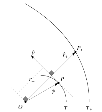
Figure 1: The map $P\rightarrow P_{*}$ and the polar reciprocal $\tau_{*}$ of $\tau$; $r_{*}=r_{\perp}^{-1}$. (The notation $\mbox{\overrightharp{$r$}}_{*}$ for $\mbox{\overrightharp{$OP$}}_{*}$ is convenient in Appendix A.)

The point $P$ is on a typical trajectory $\tau$ of a body in an (attractive) central force field (with center $O$); of course, $\tau$ is in the plane through $O$ perpendicular to $C$ (and so are $r$ and $\nu$). By construction, the vector $\mbox{\overrightharp{$OP$}}_{*}$ (in this plane) is perpendicular to the velocity $\nu$ at $P$ and has magnitude $|\mbox{\overrightharp{$OP$}}_{*}|=r_{\perp}^{-1}$. Since $r_{\perp}^{-1}=\nu/C$ [from Eq. (1)] and the direction of $\mbox{\overrightharp{$OP$}}_{*}$ is obtained from that of $\nu$ by a clockwise rotation through $90^{\circ}$ (see Fig. 1), the curve $\tau_{*}$ in Fig. 1, which is the locus of points $P_{*}$ as $P$ varies over $\tau$, is the hodograph of $\tau$, rescaled by a factor of $C^{-1}$ and rotated clockwise through 90^∘ (see also section 3 of Ref. Chakerian, ). Following Ref. Chakerian, , I will term $\tau_{*}$ the polar reciprocal of $\tau$.

It is the inverse of the mapping $P\rightarrow P_{*}$ in Fig. 1 which can be used to draw trajectories. In fact, there is a pleasing symmetry. The mapping $P\rightarrow P_{*}$ is involutory, i.e. $(P_{*})_{*}=P\,$ (see Appendix A for an elementary proof), so trajectories in a central force field and their hodographs (after rotation and rescaling as in the preceding paragraph) are polar reciprocals of each other. The point-by-point determination of a trajectory from a rotated and rescaled hodograph involves exactly the steps depicted in Fig. 1.Anosov Unlike the methods of Refs. Derbes, and SalasBrito, , polar reciprocation is valid for any smooth hodograph associated with any central force field. Be that as it may, I will now specialize to orbits of the Kepler problem. I will also use the identity

$$\mbox{\overrightharp{$OP$}}_{*}=\mbox{\overrightharp{$\nu$}}\times\mbox{\overrightharp{$C$}}/C^{2},$$ (2)

which takes advantage of the fact that, for the trajectory $\tau$ depicted in Fig. 1, $C$ points perpendicularly out of the page, so that $\mbox{\overrightharp{$\nu$}}\times\mbox{\overrightharp{$C$}}$ is parallel to $\mbox{\overrightharp{$OP$}}_{*}$ and has magnitude $\nu\,C$.

For an inverse-square force per unit mass of $-\gamma\mbox{\overrightharp{$r$}}/r^{3}$ ($\gamma>0$), the equation of motion for the position vector $\mbox{\overrightharp{$OP$}}_{*}$ of a typical point $P_{*}$ on the polar reciprocal of an orbit (see Fig. 1) reads

$$\frac{d\ }{dt}\mbox{\overrightharp{$OP$}}_{*}=\frac{d\mbox{\overrightharp{$\nu$}}}{dt}\times\frac{\mbox{\overrightharp{$C$}}}{C^{2}}=-\frac{\gamma}{Cr^{2}}\,\widehat{e}_{r}\times\frac{\mbox{\overrightharp{$C$}}}{C}=+\frac{\gamma}{C^{2}}\frac{d\phi}{dt}\,\widehat{e}_{\phi}=\rho\frac{d\widehat{e}_{r}}{dt},$$ (3)

where $\rho\equiv\gamma/C^{2}$ and plane polar coordinates $r$ and $\phi$ have been adopted for the orbital plane; the corresponding unit vectors are $\widehat{e}_{r}$ and $\widehat{e}_{\phi}$ with the origin of the coordinate system at the force center $O$, and the azimuthal angle $\phi$ defined as in Fig. 2 (so that $\mbox{\overrightharp{$C$}}=r^{2}\dot{\phi}\widehat{k}$).

Figure 2: A typical point $P_{**}$ on the polar reciprocal of $k_{*}$; $\angle P_{*}OP_{**}=\phi-\phi_{*}$ as $O_{*}P_{*}\parallel OP_{**}$. By construction, $OP_{**}=OQ^{-1}=[OP_{*}\cos(\widehat{P_{*}OP_{**}})]^{-1}$ just as, in Fig. 1, $OP_{*}=[OP\cos(\widehat{POP_{*}})]^{-1}$.

Equation (3) implies that $\mbox{\overrightharp{$OP$}}_{*}-\rho\widehat{e}_{r}$ is a (vectorial) constant of the motion, say $\mbox{\overrightharp{$OO$}}_{*}$ (drawn in Fig. 2). Setting $\mbox{\overrightharp{$OO$}}_{*}=\rho{\mbox{\overrightharp{$\varepsilon$}}}_{*}$,

$$\mbox{\overrightharp{$OP$}}_{*}=\rho(\mbox{\overrightharp{$\varepsilon$}}_{*}+\widehat{e}_{r}),$$ (4)

which demonstrates that the polar reciprocal $k_{*}$ of an orbit $k$ of the Kepler problem is a circle or an arc of a circle (as suggested by the plot in Fig. 2).Vivarelli

The polar reciprocal of $k_{*}$ (which would be the corresponding orbit $k$) comprises points like $P_{**}$ in Fig. 2, the image (under polar reciprocation) of $P_{*}$ on $k_{*}$. In terms of the angles in Fig. 2, $r=OP_{**}=1/OQ=[OP_{*}\cos(\phi-\phi_{*})]^{-1}=(\mbox{\overrightharp{$OP$}}_{*}\cdot\widehat{e}_{r})^{-1}$ or, evaluating $\mbox{\overrightharp{$OP$}}_{*}\cdot\widehat{e}_{r}$ with Eq. (4),

$$\frac{1}{r}=\rho(\mbox{\overrightharp{$\varepsilon$}}_{*}\cdot\widehat{e}_{r}+1)=\rho(1+|\mbox{\overrightharp{$\varepsilon$}}_{*}|\cos\phi).$$ (5)

Comparison of Eq. (5) with the standard equationCoxeter for a conic in polar coordinates confirms that $P_{**}$ is on a conic with focus $O$, eccentricity $e=|\mbox{\overrightharp{$\varepsilon$}}_{*}|$, latus rectum $2/\rho$, and directrix perpendicular to $OO_{*}$. The angle $\phi$ can thus be identified as the true anomaly (of celestial mechanics), and $\mbox{\overrightharp{$\varepsilon$}}_{*}$ can be reinterpreted as a vector of magnitude equal to the eccentricity $e$ of the orbit $k$, directed from the force center $O$ to the point on $k$ of closest approach (i.e. the periapse). In fact, to within a constant, $\mbox{\overrightharp{$\varepsilon$}}_{*}$ is the Laplace-Runge-Lenz vector.Goldstein

In the previous two paragraphs, it has been shown that it is easy to establish the character of the polar reciprocal $k_{*}$ of an orbit $k$ of the Kepler problem and even easier to infer from $k_{*}$ that the orbit $k$ must be a conic section. It is now possible to indicate how, as an alternative to the methods of Refs. Derbes, and SalasBrito, , polar reciprocation may be used, in principle, to draw orbits with a compass and ruler.

Suppose that the orbiting body’s velocity is given at some point $P_{0}$ on the orbit (which need not coincide with an apse of the orbit); let $\mbox{\overrightharp{$r$}}_{0}$ be the position vector of $P_{0}$ relative to $O$, and let the associated velocity (in the rest frame of $O$) be $\mbox{\overrightharp{$\nu$}}_{0}$. First, one must construct $k_{*}$. The following sequence of steps can be employed (${P_{0}}_{*}$ below denotes the image under polar reciprocation of $P_{0}$):

• calculate $C=|\mbox{\overrightharp{$r$}}_{0}\times\mbox{\overrightharp{$\nu$}}_{0}|$ and then $\rho\,(=\gamma C^{-2})$;

• add graphically the vectors ${\mbox{\overrightharp{$OP$}}_{0}}_{*}=\mbox{\overrightharp{$\nu$}}_{0}\times\mbox{\overrightharp{$C$}}/C^{2}$ and $\mbox{\overrightharp{${P_{0}}_{*}O$}}_{*}=-(\rho/r_{0})\mbox{\overrightharp{$r$}}_{0}$ to find the position of $O_{*}$ relative to $O$;

• determine the eccentricity $e\,(=OO_{*}/\rho)$;

• at $O_{*}$, draw a circle of radius $\rho$ if $e<1$ or a circular arc on which the points $P_{*}$ are such that $|\angle OO_{*}P_{*}|>\cos^{-1}e^{-1}$ if $e\geq 1$ (cf. Fig. 3 in Appendix B).AppendixB

From a point $P_{*}$ on $k_{*}$, the corresponding point $P_{**}$ on $k$ can be determined by demanding that $\mbox{\overrightharp{$OP$}}_{**}$ is parallel to $\mbox{\overrightharp{$O_{*}P$}}_{*}$ and has magnitude $|\mbox{\overrightharp{$OP$}}_{**}|=1/OQ$. Well-known compass-and-ruler constructions suffice. One can:

• erect at $P_{*}$ a line $(l_{\perp})$ perpendicular to the line through $O_{*}P_{*}$;

• draw through $O$ the line $(l_{\|})$ parallel to the line segment $O_{*}P_{*}$, and then;

• invert the point of intersection of $l_{\perp}$ and $l_{\|}$ (the point $Q$ in Fig. 2) with respect to the unit circle centered on $O$.

Compass-and-ruler implementations (with JavaSketchpad) of all three of these procedures can be found at $<$http://www.susqu.edu/brakke/constructions/constructions.htm$>$ (accessed July 2, 2011).WallaceWest

For students today, who have access to programs like Mathematica, it may seem that there is little or no need for the geometrical construction under discussion; it takes only a few keystrokes (as in Example 2.1.9 of Ref. Tam, ) to generate a plot of a Kepler problem orbit; I have, nevertheless, witnessed the intellectual satisfaction students experience in being able to correctly anticipate the character and orientation of an orbit: these features can be deduced from initial conditions via steps (i) to (iii) of the preceding paragraph. A more traditional alternative would be to use the Laplace-Runge-Lenz vector, but I have found that even my most talented and dedicated junior-level students are somewhat mystified by this construct and disinclined to use it, when it is introduced in isolation (as it usually is) as a single-valued combination of dynamical variables which happens to be a constant of the motion. My students have been more receptive to this “exotic” constant of the motion when it is presented within the context of a discussion of hodographs or polar reciprocals of the Kepler problem. Other more mundane issues can be tackled. Some suggestions for problems are given in Appendix B.

Appendix A PROOF THAT $\bm{P_{**}}\bm{=}\bm{P}$ IN A CENTRAL FORCE FIELD

The proof below involves some elementary vector algebra and, crucially, use of the equations of motion, which can be assumed to be of the form

$$\ddot{\mbox{\overrightharp{$r$}}}=f(r)\mbox{\overrightharp{$r$}},$$ (6)

where $\mbox{\overrightharp{$r$}}(t)=x(t)\widehat{\imath}+y(t)\widehat{\jmath}$ is the position of the orbiting body relative to the force center (the orbital plane is taken the $xy$-plane with the $z$-axis parallel to the angular momentum per unit mass $C$).

By definition, under polar reciprocation, the point $P$ with position vector $\mbox{\overrightharp{$r$}}(t)$ (on trajectory $\tau$) is mapped to the point $P_{*}$ (on $\tau_{*}$) with position vector $\mbox{\overrightharp{$r$}}_{*}(t)=\dot{\mbox{\overrightharp{$r$}}}(t)\times\mbox{\overrightharp{$C$}}/C^{2}$, where $\mbox{\overrightharp{$C$}}=\mbox{\overrightharp{$r$}}(t)\times\dot{\mbox{\overrightharp{$r$}}}(t)$. Likewise, under polar reciprocation, $P_{*}$ is mapped to the point $P_{**}$ with position vector $\mbox{\overrightharp{$r$}}_{**}=\dot{\mbox{\overrightharp{$r$}}}_{*}(t)\times\mbox{\overrightharp{$C$}}_{*}/C_{*}^{2}$, where $\mbox{\overrightharp{$C$}}_{*}=\mbox{\overrightharp{$r$}}_{*}(t)\times\dot{\mbox{\overrightharp{$r$}}}_{*}(t)$.

Substituting $\mbox{\overrightharp{$r$}}(t)=x(t)\widehat{\imath}+y(t)\widehat{\jmath}$ into the definition of $\mbox{\overrightharp{$r$}}_{*}$, one finds that

$$\mbox{\overrightharp{$r$}}_{*}(t)=\left[\dot{y}(t)\widehat{\imath}-\dot{x}(t)\widehat{\jmath}\,\right]/C,$$ (7)

where $C=x(t)\dot{y}(t)-y(t)\dot{x}(t)$ ($>0$). Using Eq. (6) and the fact that $C$ is a constant of the motion, $\dot{\mbox{\overrightharp{$r$}}}_{*}$ can be simplified to

$$\dot{\mbox{\overrightharp{$r$}}}_{*}(t)=f(r)\left[y(t)\widehat{\imath}-x(t)\widehat{\jmath}\,\right]/C,$$ (8)

and, hence,

$$\mbox{\overrightharp{$C$}}_{*}=-f(r)\widehat{k}/C.$$ (9)

Equations (8) and (9) imply that $\dot{\mbox{\overrightharp{$r$}}}_{*}(t)\times\mbox{\overrightharp{$C$}}_{*}=C_{*}^{2}\,\mbox{\overrightharp{$r$}}$ or $\mbox{\overrightharp{$r$}}_{**}=\mbox{\overrightharp{$r$}}$ (as required).

Appendix B SUGGESTED PROBLEMS

(1) It is not unusual to see the orbital plane (or $xy$-plane) identified with the complex plane (or $z$-plane) via the (obvious) isomorphism $(x,y)\rightarrow z=x+iy$. Formulate polar reciprocation as an operation in the complex plane. Use this representation to prove polar reciprocation is involutory.DEliseo
(2) The polar reciprocal $k_{*}$ of a known orbit $k$ of the Kepler problem can be easily found. a) Justify the claim that the images under polar reciprocation of just two points on $k$ suffice to fix $k_{*}$.
b) Show that, with the $x$-axis aligned along $\mbox{\overrightharp{$\varepsilon$}}_{*}$, the velocity at points around $k$ is

$$\mbox{\overrightharp{$\nu$}}=(\gamma\rho)^{\frac{1}{2}}(e\,\widehat{\jmath}+\widehat{e}_{\phi})$$ (10)

in the notation of this paper.
c) By considering the periapse $A$ of $k$ (where $\mbox{\overrightharp{$\nu$}}_{A}\perp\mbox{\overrightharp{$r$}}_{A}$ and $\mbox{\overrightharp{$r$}}_{A}\parallel\mbox{\overrightharp{$\varepsilon$}}_{*}$), demonstrate that the energy $E$ of the orbiting body is related to the eccentricity $e$ of $k$ by

$$\frac{E}{m}={\textstyle\frac{1}{2}}\gamma\rho(e^{2}-1),$$ (11)

where $m$ is the mass of the orbiting body. (Begin by finding expressions for $r_{A}^{-1}=\nu_{A}/C$ and $\nu_{A}$ in terms of $\rho$ and $e$.)
d) Use Eqs. (10) and (11) to prove that the inequality $\nu^{2}\ \left(=2E/m+2\gamma/r\right)>2E/m$ reduces to $e\cos\phi>-1$.
(3) The polar reciprocal of an elliptical orbit (of the Kepler problem) must be a complete circle (as opposed to only an arc of a circle) because of the periodicity of the motion. Show that this circle has radius

$$\rho=\frac{1}{2}\left(\frac{1}{r_{p}}+\frac{1}{r_{a}}\right),$$ (12)

where $r_{p}$ and $r_{a}$ are the distances (from the force center $O$) of the periapse and apoapse, respectively, and that the distance of its center $O_{*}$ from $O$ is

$$OO_{*}=\frac{1}{2}\left(\frac{1}{r_{p}}-\frac{1}{r_{a}}\right).$$ (13)

Infer from Eqs. (12) and (13) an expression for the eccentricity of the orbit.

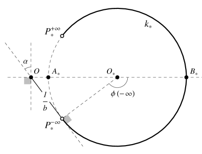
Figure 3: The polar reciprocal $k_{*}$ of the hyperbolic orbit $k$ of Fig. 4. The point $B_{*}$ is the image under polar reciprocation of point $B$ in Fig. 4; $P^{\pm\infty}_{*}$ are the images of the two points at infinity $P^{\pm\infty}=\lim_{t\rightarrow\pm\infty}P(t)$ on the in/out asymptotes. Like $k$, $k_{*}$ is symmetric about the principal axis of $k$ (the line through $O$ and $O_{*}$).

(4) Figure 3 depicts the polar reciprocal $k_{*}$ of the hyperbolic orbit $k$ in Fig. 4. Prove that $OP_{*}^{-\infty}$ is tangent to the circle in Fig. 3 of which $k_{*}$ is a part by showing that $\angle OP_{*}^{\pm\infty}O_{*}=90^{\circ}$. By appealing to the “tangent-secant theorem”,Euclid deduce that $OA_{*}=r_{B}/b^{2}$. Hence, conclude that, in Fig. 3, the circle has radius

$$\rho=\frac{1}{2r_{B}}\left(1-\frac{r_{B}^{2}}{b^{2}}\right)$$ (14)

and

$$OO_{*}=\frac{1}{2r_{B}}\left(1+\frac{r_{B}^{2}}{b^{2}}\right).$$ (15)

Use Eqs. (14) and (15) to justify the assertion that results appropriate to parabolic orbits can be obtained by taking the limit $b\rightarrow\infty$, keeping $r_{B}$ fixed.

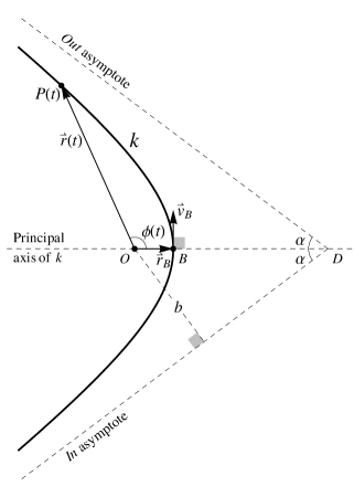
Figure 4: A hyperbolic orbit $k$ of the Kepler problem.

(5) Many spacecraft maneuvers involve short firings of high-thrust rockets, which can be modeled as resulting in instantaneous changes $\Delta\mbox{\overrightharp{$\nu$}}$ in velocity with no change in position. The important Hohmann transfer (depicted in Fig. 5) requires two such impulsive thrusts: the first (at $P_{i}$) places the vehicle on the semi-elliptical trajectory $h_{if}$, and the second (at $P_{f}$) puts the vehicle into the circular orbit $c_{f}$.Gregory

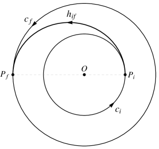
Figure 5: The Hohmann transfer trajectory $h_{if}$ between coplanar circular orbits $c_{i}$ and $c_{f}$ in the field of a spherical mass centered on $O$; $h_{if}$ is tangent to $c_{i}$ at $P_{i}$ and tangent to $c_{f}$ at $P_{f}$.

a) Show that, provided $\Delta\mbox{\overrightharp{$\nu$}}$ is tangential to the spacecraft’s orbit and the direction of motion of the spacecraft is not reversed, $\mbox{\overrightharp{$r$}}_{*}=\mbox{\overrightharp{$\nu$}}\times\mbox{\overrightharp{$C$}}/C^{2}$ is unchanged by an impulsive thrust.
b) Find the polar reciprocal representation of the Hohmann transfer in Fig. 5, i.e. draw (in one diagram) the polar reciprocals of $c_{i}$, $c_{f}$, and $h_{if}$.
c) Generalize the result of part b) to the case of two counter-clockwise non-intersecting co-planar and co-axial elliptical orbits about the force center $O$. The transfer trajectory must connect the periapse of the inner orbit to the apoapse of the outer orbit.

References

- (1) H. Abelson, A. diSessa and L. Rudolph, “Velocity space and the geometry of planetary orbits,” Am. J. Phys. 43, 579-589 (1975).
- (2) A. González-Villanueva, H. N. Núñez-Yépez, and A. L. Salas-Brito, “In veolcity space the Kepler orbits are circular,” Eur. J. Phys. 17, 168-171 (1996).
- (3) T. A. Apostolatos, “Hodograph: A useful geometrical tool for solving some difficult problems in dynamics,” Am. J. Phys. 71, 261-266 (2003).
- (4) E. I. Butikov, “Comment on ‘Eccentricity as a vector’,” Eur. J. Phys. 25, L41-L43 (2004).
- (5) C. I. Mungan, “Another comment on ‘Eccentricity as a vector’,” Eur. J. Phys. 26, L7-L9 (2005).
- (6) D. L. Goodstein and J. R. Goodstein, Feynman’s Lost Lecture: The Motion of Planets Around the Sun (W. W. Norton, New York, 1996).
- (7) G. W. Griffiths, Math. Intelligencer 20 (3), 68-70 (1998), review of Ref. FLL, .
- (8) R. Weinstock, Math. Intelligencer 21 (3), 71-73 (1999), review of Ref. FLL, .
- (9) D. Derbes, “Reinventing the wheel: Hodographic solutions to the Kepler problems,” Am. J. Phys. 69, 481-489 (2001).
- (10) E. Guillaumin-España, A. L. Salas-Brito, and H. N. Núñez-Yépez, “Tracing a planet’s orbit with a straight edge and a compass with the help of the hodograph and the Hamilton vector,” Am. J. Phys. 71, 585-589 (2003).
- (11) D. W. Tiberiis, “Comment on ‘Reinventing the wheel: Hodographic solutions to Kepler problems,’ by David Derbes [Am. J. Phys. 69(4), 481-489 (2001)],” Am. J. Phys. 70, 79 (2002).
- (12) I. Newton, Philosophiae Naturalis Principia Mathematica (University of California Press, Berkeley, CA, 1934) translation (into English) by Motte (revised by Cajori).
- (13) D. Chakerian, “Central Force Laws, Hodographs, and Polar Reciprocals,” Mathematics Magazine 74, 3-18 (2001).
- (14) Trajectories for which have to be excluded, but these are one-dimensional and easily drawn once the initial conditions are known. See D. V. Anosov, “A note on the Kepler problem,” J. Dynamical and Control Systems 8, 413-442 (2002).
- (15) Equation (4) is implicit in the existing literature on hodographs. For example, Eq. (4) can be inferred from Eq. (3) of Ref. Butikov, , which is a concise and extremely clear treatment of hodographs for the Kepler problem. Algebraic considerations specific to the Kepler problem are used to motivate the introduction of a sum vector \overrightharp, which is exactly the combination of vectors in Eq. (4), in M. D. Vivarelli, “A configuration counterpart of the Kepler problem hodograph,” Celestial Mechanics and Dynamical Astronomy 68, 305-311 (1998).
- (16) H. S. M. Coxeter, Introduction to Geometry, 2nd ed. (John Wiley & Sons, New York, 1969).
- (17) This result could also have been established directly by using the fact that to recast Eq. (4) as the relation , where is the mass of the orbiting particle and \overrightharp is the Laplace-Runge-Lenz vector as defined in H. Goldstein, Classical Mechanics, 2nd ed. (Addison-Wesley, Reading, MA, 1980).
- (18) Part d) of Problem 2 in Appendix B addresses the origin of this angular restriction on for .
- (19) The hyperlink on this web page to last of these three operations appears between hyperlinks 29 and 30 (and directs one to the web page http://www.susqu.edu/brakke/constructions/InversionTool.htm); the hyperlinks (numbered 3 and 8) to the other two operations are more obvious. A less ephemeral source for all of these constructions is E. C. Wallace and S. F. West, Roads to Geometry, 2nd ed. (Prentice-Hall, Upper Saddle River, NJ, 1998), which deals with inversion of a point in the unit circle on p. 278, and the other two constructions on pp. 191-2.
- (20) P. T. Tam, A Physicist’s Guide to Mathematica, 2nd ed. (Academic Press, Burlington, MA, 2008).
- (21) Other applications of the complex variable formalism to central force problems appear in M. M. D’Eliseo, “The first-order orbital equation,” Am. J. Phys. 75, 352-355 (2007).
- (22) Alternatively, Euclid’s proposition III.36 on secants of a circle (stated on page 8 in Ref. Coxeter, ).
- (23) A brief but usually careful introduction to the Hohmann transfer of Fig. 5 is given in section 7.6 of R. D. Gregory, Classical Mechanics (Cambridge University Press, Cambridge, 2006).