Role of diversification risk in financial bubbles

Abstract

We present an extension of the Johansen-Ledoit-Sornette (JLS) model to include an additional pricing factor called the “Zipf factor”, which describes the diversification risk of the stock market portfolio. Keeping all the dynamical characteristics of a bubble described in the JLS model, the new model provides additional information about the concentration of stock gains over time. This allows us to understand better the risk diversification and to explain the investors’ behavior during the bubble generation. We apply this new model to two famous Chinese stock bubbles, from August 2006 to October 2007 (bubble 1) and from October 2008 to August 2009 (bubble 2). The Zipf factor is found highly significant for bubble 1, corresponding to the fact that valuation gains were more concentrated on the large firms of the Shanghai index. It is likely that the widespread acknowledgement of the 80-20 rule in the Chinese media and discussion forums led many investors to discount the risk of a lack of diversification, therefore enhancing the role of the Zipf factor. For bubble 2, the Zipf factor is found marginally relevant, suggesting a larger weight of market gains on small firms. We interpret this result as the consequence of the response of the Chinese economy to the very large stimulus provided by the Chinese government in the aftermath of the 2008 financial crisis.

I Introduction

Johansen et al. js ; jsl ; jls developed a model (referred to below as the JLS model) of financial bubbles and crashes, which is an extension of the rational expectation bubble model of Blanchard and Watson Blanchardwat . In this model, a crash is seen as an event potentially terminating the run-up of a bubble. A financial bubble is modeled as a regime of accelerating (super-exponential power law) growth punctuated by short-lived corrections organized according to the symmetry of discrete scale invariance DSI-sornette98 . The super-exponential power law is argued to result from positive feedback resulting from noise trader decisions that tend to enhance deviations from fundamental valuation in an accelerating spiral.

The JLS model has been proved to be a very powerful and flexible tool to detect financial bubbles and crashes in various kinds of markets such as the 2006 - 2008 oil bubble oil , the Chinese index bubble in 2009 Jiangetal09 , the real estate market in Las Vegas vegas , the South African stock market bubble southafrica and the US repurchase agreement market repo . Recently, the JLS model has been extended to detect market rebounds rebound and to infer the fundamental market value hidden within observed prices pp1 . Also, new experiments in ex-ante bubble detection and forecast has been performed in the Financial Crisis Observatory at ETH Zurich BFEFCO09 ; BFEFCO10 .

Here, we present an extension of the JLS model, which is in the spirit of the approach developed by Zhou and Sornette zhouSornette06 to include additional pricing factors.

The literature on factor models is huge and we refer e.g. to Ref.KnightSatchell and references therein for a review of the literature. One of the most famous factor model, now considered as a standard benchmark, is the three-factor Fama-French model FamaandFrench1992 ; FamaandFrench1993 ; FamaandFrench1995 ; FamaandFrench1996 augmented by the momentum factor Carhart1997 . Recently, the concept of the Zipf factor has been introduced MalevergneSortwofactor ; MalevergneSantaSor . The key idea of the Zipf factor is that, due to the concentration of the market portfolio when the distribution of the capitalization of firms is sufficiently heavy-tailed as is the case empirically, a risk factor generically appears in addition to the simple market factor, even for very large economies. Malevergne et al. MalevergneSortwofactor ; MalevergneSantaSor proposed a simple proxy for the Zipf factor as the difference in returns between the equal-weighted and the value-weighted market portfolios. Malevergne et al. MalevergneSortwofactor ; MalevergneSantaSor have shown that the resulting two-factor model (market portfolio $+$ the new factor termed “Zipf factor”) is as successful empirically as the three-factor Fama-French model. Specifically, tests of the Zipf model with size and book-to-market double-sorted portfolios as well as industry portfolios finds that the Zipf model performs practically as well as the Fama-French model in terms of the magnitude and significance of pricing errors and explanatory power, despite that it has only two factors instead of three.

In the present paper, we would like to introduce a new model by combining the Zipf factor with the JLS model. The new model keeps all the dynamical characteristics of a bubble described in the JLS model. In addition, the new model can also provide the information about the concentration of stock gains over time from the knowledge of the Zipf factor. This new information is very helpful to understand the risk diversification and to explain the investors’ behavior during the bubble generation.

The paper is constructed as follows. Section II describes the definition of the Zipf factor as well as the new model. The derivation of the model is presented in this section and the appendix. Section III introduces the calibration method of this new model. Then we test the new model with two famous Chinese stock bubbles in the history in Section IV and discuss the role of the Zipf factor in these two bubbles. Section V concludes.

II The model

We introduce the new model in this section. Our goal is to combine the Zipf factor $z(t)dt$ with the JLS model of the bubble dynamics. To be specific, we introduce the following definition.

Definition 1: The Zipf factor $z(t)dt$ is defined as proportional to the difference between the returns of the capitalization-weighted portfolio and the equal-weighted portfolio for the last time step:

$$z(t)dt:=\frac{dp}{p(t)}-\frac{dp_{e}}{p_{e}(t)}~{},$$ (1)

where $p$ (respectively $p_{e}$) is the price of the capitalization-weighted (respectively equal-weighted) portfolio, $dp:=p(t)-p(t-dt)$ and $dp_{e}:=p_{e}(t)-p_{e}(t-dt)$. The weights of the portfolios are normalized so that their two prices are identical at the day preceding the beginning time $t_{0}$ of the time series: $p_{e}(t_{0})=p(t_{0})$.

Definition 2: The integrated Zipf factor $\zeta(t)$ is obtained by taking the integral of the Zipf factor defined by expression (1):

$$\zeta(t):=\ln p(t)-\ln p_{e}(t)~{}.$$ (2)

By definition, the Zipf factor describes the exposition to a lack of diversification due to the concentration of the stock market on a few very large firms.

The dynamics of stock markets during a bubble regime is then described as

$$\frac{dp(t)}{p(t)}=\mu(t)dt+\gamma z(t)dt+\sigma(t)dW-\kappa dj~{},$$ (3)

where $p$ is the portfolio price, $\mu$ is the drift (or trend) whose accelerated growth describes the presence of a bubble (see below), $\gamma$ is the factor loading on the Zipf’s factor and $dW$ is the increment of a Wiener process (with zero mean and unit variance). The term $dj$ represents a discontinuous jump such that $dj=0$ before the crash and $dj=1$ after the crash occurs. The loss amplitude associated with the occurrence of a crash is determined by the parameter $\kappa$. The assumption of a constant jump size is easily relaxed by considering a distribution of jump sizes, with the condition that its first moment exists. Then, the no-arbitrage condition is expressed similarly with $\kappa$ replaced by its mean. Each successive crash corresponds to a jump of $dj$ by one unit. The dynamics of the jumps is governed by a crash hazard rate $h(t)$. Since $h(t)dt$ is the probability that the crash occurs between $t$ and $t+dt$ conditional on the fact that it has not yet happened, we have $E_{t}[dj]=1\times h(t)dt+0\times(1-h(t)dt)$, where $E_{t}[.]$ denotes the expectation operator. This leads to

$${\rm E}_{t}[dj]=h(t)dt~{}.$$ (4)

Noise traders exhibit collective herding behaviors that may destabilize the market in this model. We assume that the aggregate effect of noise traders can be accounted for by the following dynamics of the crash hazard rate

$$h(t)=B^{\prime}(t_{c}-t)^{m-1}+C^{\prime}(t_{c}-t)^{m-1}\cos(\omega\ln(t_{c}-t)-\phi^{\prime})~{}.$$ (5)

The intuition behind this specification (5) has been presented at length by Johansen et al. js ; jsl ; jls , and further developed by Sornette and Johansen SorJohansenQF01 , Ide and Sornette IdeSornette and Zhou and Sornette zhouSornette06 . In a nutshell, the power law behavior $\sim(t_{c}-t)^{m-1}$ embodies the mechanism of positive feedback posited to be at the source of the bubbles. If the exponent $m<1$, the crash hazard may diverge as $t$ approaches a critical time $t_{c}$, corresponding to the end of the bubble. The cosine term in the r.h.s. of (5) takes into account the existence of a possible hierarchical cascade of panic acceleration punctuating the course of the bubble, resulting either from a preexisting hierarchy in noise trader sizes SornetteJohansen97 and/or from the interplay between market price impact inertia and nonlinear fundamental value investing IdeSornette .

We assume that all the investors of the market have already taken the diversification risk into account, so that the no-arbitrage condition reads ${\rm E}_{t}[\frac{dp(t)}{p(t)}-\gamma z(t)dt]=0$, where the expectation is performed with respect to the risk-neutral measure, and in the frame of the risk-free rate. This is the condition that the price process concerning the diversification risk should be a martingale. Taking the expectation of expression (3) under the filtration (or history) until time $t$ reads

$${\rm E}_{t}\left[\frac{dp}{p}-\gamma zdt\right]=\mu(t)dt+\sigma(t){\rm E}_{t}[dW]-\kappa{\rm E}_{t}[dj]~{}.$$ (6)

Since ${\rm E}_{t}[dW]=0$ and ${\rm E}_{t}[dj]=h(t)dt$ (equation (4)), together with the no-arbitrage condition ${\rm E}_{t}[dp(t)]=0,\forall t$, this yields

$$\mu(t)=\kappa h(t)~{}.$$ (7)

This result (7) expresses that the return $\mu(t)$ is controlled by the risk of the crash quantified by its crash hazard rate $h(t)$. The excess return $\mu(t)=\kappa h(t)$ is the remuneration that investors require to remain invested in the bubbly asset, which is exposed to a crash risk.

Now, conditioned on the fact that no crash occurs, equation (3) is simply

$$\frac{dp(t)}{p(t)}-\gamma z(t)=\mu(t)dt+\sigma(t)dW=\kappa h(t)dt+\sigma(t)dW~{},$$ (8)

where the Zipf factor $z(t)$ is given by expression (1). Its conditional expectation leads to

$${\rm E}_{t}\left[\frac{dp(t)}{p(t)}-\gamma z(t)\right]=\kappa h(t)dt$$ (9)

Substituting with the expression (5) for $h(t)$ and (1) for $z(t)$, and integrating, yields the log-periodic power law (LPPL) formula as in the JLS model, but here augmented by the presence of the Zipf factor, which adds the term proportional to the Zipf factor loading $\gamma$:

$${\rm E}_{t}[\ln p(t)-\gamma\zeta(t)]=A+B(t_{c}-t)^{m}+C(t_{c}-t)^{m}\cos(\omega\ln(t_{c}-t)-\phi)~{},$$ (10)

where $\zeta(t)$ is defined by expression (2) and the r.h.s. of (10) is the primitive of expression (5) so that $B=-\kappa B^{\prime}/m$ and $C=-\kappa C^{\prime}/\sqrt{m^{2}+\omega^{2}}$. This expression (10) describes the average price dynamics only up to the end of the bubble. The same structure as equation (10) is obtained using a stochastic discount factor following the derivation of Zhou and Sornette zhouSornette06 , as shown in the appendix.

The JLS model does not specify what happens beyond $t_{c}$. This critical $t_{c}$ is the termination of the bubble regime and the transition time to another regime. This regime could be a big crash or a change of the growth rate of the market. Merrill Lynch EMU (European Monetary Union) Corporates Non-Financial Index in 2009 BFE-FCO09 provides a vivid example of a change of regime characterized by a change of growth rate rather than by a crash or rebound. For $m<1$, the crash hazard rate accelerates up to $t_{c}$ but its integral up to $t$ which controls the total probability for a crash to occur up to $t$ remains finite and less than $1$ for all times $t\leq t_{c}$. It is this property that makes it rational for investors to remain invested knowing that a bubble is developing and that a crash is looming. Indeed, there is still a finite probability that no crash will occur during the lifetime of the bubble. The condition that the price remains finite at all time, including $t_{c}$, imposes that $m>0$.

Within the JLS framework, a bubble is qualified when the crash hazard rate accelerates. According to (5), this imposes $m<1$ and $B^{\prime}>0$, hence $B<0$ since $m>0$ by the condition that the price remains finite. We thus have a first condition for a bubble to occur

$$0<m<1~{}.$$ (11)

By definition, the crash rate should be non-negative. This imposes bm

$$b\equiv-Bm-|C|\sqrt{m^{2}+\omega^{2}}\geq 0~{}.$$ (12)

III Calibration method

There are eight parameters in this LPPL model augmented by the introduction of the Zipf’s factor, four of which are the linear parameters ($\gamma,A,B$ and $C$). The other four ($t_{c},m,\omega$ and $\phi$) are nonlinear parameters.

We first slave the linear parameters to the nonlinear ones. The method here is the same as used by Johansen et al. jls . The detailed equations and procedure is as follows. We rewrite Eq. (10) as:

$${\rm E}[\ln p(t)]=\gamma\zeta(t)+A+Bf(t)+Cg(t):=RHS(t)~{}.$$ (13)

We have also defined

$$f(t)=(t_{c}-t)^{m}~{},~{}~{}~{}~{}~{}g(t)=(t_{c}-t)^{m}\cos(\omega\ln(t_{c}-t)-\phi)~{}.$$ (14)

The minimization of the sum of the squared residuals should satisfy

$$\frac{\partial\Sigma_{t}[\ln p(t)-RHS(t)]^{2}}{\partial\theta}=0,~{}~{}~{}\forall~{}\theta\in\{\gamma,A,B,C\}.$$ (15)

The linear parameters $\gamma,A,B$ and $C$ are determined as the solutions of the linear system of four equations:

$$\Sigma_{t=t_{1}}^{t_{2}}\left(\begin{array}[]{cccc}\zeta^{2}(t)&\zeta(t)&\zeta(t)f(t)&\zeta(t)g(t)\\ \zeta(t)&1&f(t)&g(t)\\ \zeta(t)f(t)&f(t)&f^{2}(t)&f(t)g(t)\\ \zeta(t)g(t)&g(t)&f(t)g(t)&g^{2}(t)\end{array}\right)\left(\begin{array}[]{c}\gamma\\ A\\ B\\ C\end{array}\right)=\Sigma_{t=t_{1}}^{t_{2}}\left(\begin{array}[]{c}\zeta(t)\ln p(t)\\ \ln p(t)\\ f(t)\ln p(t)\\ g(t)\ln p(t)\end{array}\right)~{}.$$ (16)

This provides four analytical expressions for the four linear parameters $(\gamma,A,B,C)$ as a function of the remaining nonlinear parameters $t_{c},m,\omega,\phi$. The resulting cost function (sum of square residuals) becomes function of just the four nonlinear parameters $t_{c},m,\omega,\phi$. This achieves a very substantial gain in stability and efficiency as the search space is reduced to the 4 dimensional parameter space $(t_{c},m,\omega,\phi)$. A heuristic search implementing the taboo algorithm ck is used to find initial estimates of the parameters which are then passed to a Levenberg-Marquardt algorithm kl ; dm to minimize the residuals (the sum of the squares of the differences) between the model and the data. The calibration is performed for the time window delineated by $[t_{1},t_{2}]$, where $t_{1}$ is the starting time and $t_{2}$ is the ending time of the price time being fitted by expression (10) or equivalently (13).

The bounds of the search space are:

$$t_{c} \in [t_{2},t_{2}+0.375(t_{2}-t_{1})]$$ (17)

$$m \in [10^{-5},1-10^{-5}]$$ (18)

$$\omega \in [0.01,40]$$ (19)

$$\phi \in [0,2\pi-10^{-5}]$$ (20)

We choose these bounds because $m$ has to be between $0$ and $1$ according to the discussion before; the log-angular frequency $\omega$ should be greater than $0$. The upper bound $40$ is large enough to catch high-frequency oscillations (though we later discard fits with $\omega>20$); the phase $\phi$ should be between 0 and $2\pi$; The predicted critical time $t_{c}$ should be after the end $t_{2}$ of the fitted time series. Finally, the upper bound of the critical time $t_{c}$ should not be too far away from the end of the time series since predictive capacity degrades far beyond $t_{2}$. Jiang et al. Jiangetal09 have found empirically that a reasonable choice is to take the maximum horizon of predictability to extent to about one-third of the size of the fitted time window.

IV Application to the Shanghai Composite Index (SSEC)

IV.1 Construction of the capitalization-weighted and equally-weighted portfolios

We use the Shanghai Composite Index as the market proxy to test the JLS model augmented with the Zipf factor. The Shanghai Composite Index is a capital-weighted measure of stock market performance. On December 19, 1990, the base value of the Shanghai Composite Index $I$ was fixed to $100$. We note the base date as $t_{B}$. Denoting by $K_{B}$, the total market capitalization of the firms entering in the Shanghai Composite index on $t_{B}$ December 19, 1990, the value $p(t)$ of the Shanghai Composite Index at any later time $t$ is given by

$$p(t)=\frac{K(t)}{K_{B}}\times 100,$$ (21)

where $K(t)$ is the current total market capitalization of the constituents of the Shanghai Composite index. Here, time is counted in units of trading days. Calling $p_{j}(t)$ (respectively $s_{j}(t)$), the share price (respectively total number of shares) of firm $j$ at time $t$, we have the total capitalization of firm $j$ at time $t$

$$K_{j}(t)=p_{j}(t)s_{j}(t)~{},$$ (22)

and the total market capitalization at time $t$

$$K(t)=\sum_{j=1}^{M(t)}K_{j}(t)~{},$$ (23)

where $M(t)$ is the number of the stocks listed in the index at time $t$.

At the time when the calibrations were performed, the SSEC market included 884 active stocks. Since December 19, 1990, 36 firms were delisted and another 11 were temporarily stopped. Based on the rule of the index calculation, the terminated stocks are deleted from the total market capitalization after the termination is executed, while the last active capitalization of the temporarily stopped stocks are still included in the total market capitalization.

The equal-weighted price $p_{e}$ entering in the definition of the Zipf factor is constructed according to the formula:

$$p_{e}(t)=p(t_{0})\times\exp\left[\sum_{i=t_{1}}^{t}r_{e}(i)\right]~{},$$ (24)

where $t_{1}$ is the beginning of the fitted window and $t_{0}$ is the trading day immediately preceding $t_{1}$. We use this measure of $p_{e}$ to make sure that the equal-weighted price and the value-weighted price are identical at $t_{0}$. This implies that $\zeta(t_{0})$ is set to be $0$ (recall that $\zeta$ is defined by expression (2)). The return $r_{e}(i)$ is defined by

$$r_{e}(i)={1\over M(i)}\sum_{j=1}^{M(i)}\left[\ln K_{j}(i)-\ln K_{j}(i-1)\right]~{}.$$ (25)

In expression (25), $K_{j}(i)$ is the total capitalization value of firm $j$ at time $i$ and $M(i)$ is the number of the stocks which are listed in the index for both time $i$ and $i-1$. Formula (25) together with (24) means that the Zipf factor is a portfolio that puts an equal amount of wealth at each time step (by a corresponding dynamical reallocation depending on the relative performance of the $M(i)$ stocks as a function of time) on each of the $M(i)$ stocks entering in the definition of the Shanghai Composite Index, so that the Zipf portfolio is maximally diversified (neglecting here the impact of cross-correlations between the assets). Putting expression (25) inside (24) yields

$$p_{e}(t)=p(t_{0})\times\prod_{i=t_{1}}^{t}\left[\left(\prod_{j=1}^{M(i)}{K_{j}(i)\over K_{j}(i-1)}\right)^{1/M(i)}\right]~{}.$$ (26)

When the number of the stocks remains unchanged from $t_{0}$ to $t$, i.e.

$$M(i)=M,~{}~{}~{}~{}~{}\forall i\in[t_{0},t]~{},$$ (27)

expression (26) can be simplified as:

$$p_{e}(t)=p(t_{0})\times\left[\prod_{j=1}^{M}\left({K_{j}(t)\over K_{j}(t_{0})}\right)\right]^{1/M}~{},$$ (28)

showing that $p_{e}(t)$ is the geometrical mean of the capitalizations of the stocks constituting the Shanghai Composite Index, as compared with the index which is proportional to the arithmetic mean of the firm capitalizations.

IV.2 Empirical test of the JLS model augmented by the Zipf factor

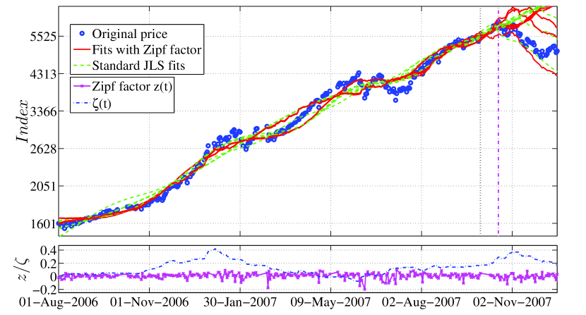
Figure 1: Calibration of the new factor model and the original JLS model to the Shanghai Composite Index (SSEC) between Aug-01-2006 and Sep-28-2007. (Upper panel) The beginning of the fit interval is the left boundary of the plot, while the end of the fit interval is indicated by the vertical thick black dotted line. The real critical time $t_{c}$ when the crash started is marked by the vertical magenta dot-dashed line. The historical close prices are shown as blue full circles. The best 10 fits of the original JLS model are shown as the green dashed lines and the best 10 fits of the new factor model are shown as the red solid lines. (Lower panel) The corresponding Zipf factor (magenta solid line with ‘x’ symbol) and $\zeta$ function (blue dot-dashed line) during this period.

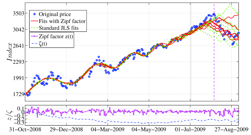
Figure 2: Calibration of the new factor model and the original JLS model to the Shanghai Composite Index (SSEC) between Oct-31-2008 and Jul-01-2009. (Upper panel) The beginning of the fit interval is the left boundary of the plot, while the end of the fit interval is indicated by the vertical thick black dotted line. The real critical time $t_{c}$ when the crash started is marked by the vertical magenta dot-dashed line. The historical close prices are shown as blue full circles. The best 10 fits of the original JLS model are shown as the green dashed lines and the best 10 fits of the new factor model are shown as the red solid lines. (Lower panel) The corresponding Zipf factor (magenta solid line with ‘x’ symbol) and $\zeta$ function (blue dot-dashed line) during this period.

The Shanghai Composite Index had two famous bubbles in recent history as described in Table 1. Both of them are tested in this paper. The time series are fitted with both the original JLS model and the new model. The 10 best initial guesses from the heuristic search algorithm are kept. The results are shown in Figs. 1 - 2.

Example	Calibration start at $t_{1}$	Prediction start at $t_{2}$	Peak date of the bubble
Bubble 1	Aug-01-2006	Sep-28-2007	16-Oct-2007
Bubble 2	Oct-31-2008	Jul-01-2009	Aug-04-2009

Table 1: Information on the tested bubbles of SSEC.

We use the standard Wilks test of nested hypotheses to check the improvement of the new factor model. This test assumes independent and normally distributed residuals. The null hypothesis is:

1. the original JLS model is sufficient and the new factor model is not necessary.

The alternative hypothesis reads:

1. The original JLS model is not sufficient and the new factor model is needed.

For sufficiently large time windows, and noting $T$ the number of trading days in the fitted time window $[t_{1},t_{2}]$, the Wilks log-likelihood ratio reads

$$W=2\log\frac{L_{Zipf,max}}{L_{JLS,max}}=2T\ln\frac{\sigma_{JLS}}{\sigma_{Zipf}}+\frac{\sum_{t=1}^{T}R_{JLS}^{2}(t)}{\sigma_{JLS}^{2}}-\frac{\sum_{t=1}^{T}R_{Zipf}^{2}(t)}{\sigma_{Zipf}^{2}}~{},$$ (29)

where $R_{JLS}$ and $\sigma_{JLS}$ (respectively $R_{Zipf}$ and $\sigma_{Zipf}$) are the residuals and their corresponding standard deviation for the original JLS model (respectively the new factor model).

In the large $T$ limit, and under the above conditions of asymptotic independence and normality, the $W$-statistics is distributed with a $\chi_{k}^{2}$ distribution with $k$ degrees of freedom, where $k$ is the difference between the number of parameters in two models. In our case, the new factor model has one more parameter, which is $\gamma$. Therefore, $W$ in Eq.(29) should follow the $\chi_{1}^{2}$ distribution.

Only considering the best fit for each of the two models, we obtain a $p$-value associated with the empirical value of the $W$-statistics equal to $2.64\times 10^{-7}$ for bubble 1 and $0.2517$ for bubble 2. Thus, the null hypothesis is rejected and the Zipf factor is necessary for the best fit of bubble 1, while the null hypothesis is not rejected and the Zipf factor is not necessary for the best fit of bubble 2. This result is also consistent with the two values found for $\gamma$, where $\gamma=0.44$ for bubble 1 and $\gamma=-0.028$ for bubble 2, showing the Zipf factor in bubble 1 plays an important role in the improvement of the fit quality.

Keeping the best 10 fits as we described before increases the statistical power of the Wilks test (simply by having more statistical data) and we want to show that the new JLS model with the Zipf factor is an significant improvement. For this, we combine all of the residuals from the best 10 fits to the data into a large residual sample and calculate the Wilks log-likelihood ratio $W$ for this large sample as defined by expression (29). The corresponding p-values are $0$ for bubble 1 and $0.0119$ for bubble 2. This means the new factor model performs better than the original JLS model for both cases when we consider the overall qualify of the best 10 fits.

A natural and interesting test is to find out if the new model with Zipf factor has a better predictability of the critical time. To achieve this goal, two examples are fitted by both models within different time windows obtained by varying their start time $t_{1}$ and the end time $t_{2}$. We consider 15 different values of $t_{1}$ and of $t_{2}$ in steps of 3 days, yielding 225 time series for each example. We keep the best 10 fits for each time series and get 2250 predicted critical time $t_{c}$ with each model and for each example. The results in Table 2 show that the mean value and the standard deviation of the critical time $t_{c}$ for both models are similar. The new model including the Zipf factor neither improves nor deteriorates the predictability of the critical time for these two examples.

Example	Peak date	Mean(std) of $t_{c}$, new model	Mean(std) of $t_{c}$, original model
Bubble 1	16-Oct-2007	07-Oct-2007(55.6)	18-Oct-2007(54.1)
Bubble 2	Aug-04-2009	04-Jul-2009(33.6)	05-Jul-2009(32.4)

Table 2: Prediction of the critical time for both models. For each example, 225 time series are generated by varying the start time $t_{1}$ and end time $t_{2}$ of the windows in which the calibration is performed. The mean value and the standard deviation of the predicted critical time $t_{c}$ among 2250 predictions are shown in the table.

However, the new model makes it possible to determine the concentration of stock gains over time from the knowledge of the Zipf factor. The two bubbles are found to differ by the sign and contribution of the Zipf factor as well as the factor load $\gamma$.

For bubble 1, the integrated Zipf factor $\zeta$ is positive as shown in Fig. 1, corresponding to the fact that valuation gains were more concentrated on the large firms of the Shanghai index, especially in two periods, Dec. 2006 - Jan. 2007 and Oct. 2007 - Dec. 2007. The factor load $\gamma$ of the best fit in the example shown in Fig. 1 is 0.44. And the statistics of $\gamma$ from all the 2250 fits of bubble 1 is shown in the second row of Tab. 3. All these results indicate that the Zipf factor load $\gamma$ in bubble 1 is statistically large and positive. This implies the existence of a lack-of-diversification premium that contributes significantly to the overall price level in addition to the bubble component.

A possible interpretation of the important of the Zipf factor is based on the importance that investors started to attribute to the role of large companies in driving the appreciation of the SSEC index during the first bubble. The so-called 80-20 rule started to be hot among investors in discussions and interpretation of the rising SSEC index. It was widely pointed out that the growth of the SSEC index was driven essentially by 20% of the stocks while the other 80% constituents of the index remains approximately flat (known as the 80-20 quotation of the Chinese stock market ). It is plausible that the widespread acknowledgement of the 80-20 rule led many investors to discount the risk of a lack of diversification, therefore enhancing the role of the Zipf factor. This is consistent with our observation that the Zipf factor load $\gamma$ is large and positive during the first bubble period.

Example	$Meanof\gamma$	Median of $\gamma$	std of $\gamma$
Bubble 1	0.35	0.56	0.43
Bubble 2	-0.14	-0.11	0.15

Table 3: Statistics of the Zipf factor load $\gamma$ from 2250 fit results. Most of the values for $\gamma$ for the period during the development of bubble 1 are positive and their average value is large. This means that the Zipf factor plays an important role during the development of bubble 1. The concentration of the stock market on a small number of large firms has a significant impact on the price change of the stock index. In contrast, for bubble 2, the average value of $\gamma$ is relatively small and the exposition to the risk associated with a lack of diversification is found to be insignificant in pricing the value of the market.

In contrast, the integrated Zipf factor $\zeta$ remained negative over the lifetime of bubble 2 as shown in Fig. 2, implying that the gains of the Shanghai index were more driven by small and medium size firms. The factor load $\gamma$ is -0.028 for the best fit shown in Fig. 2 and the mean value of $\gamma$ for bubble 2 is small and negative (see Tab. 3). The overall contribution of the Zipf factor to the stock change is therefore small and negative (due to the product of a negative integrated Zipf factor by a negative factor loading), which makes the remuneration of investors due to their exposition to the diversification risk still positive but small.

At the time when bubble 2 started, the world economy has been seriously shaken by the developing subprime crisis. The demand for Chinese product exports decreased dramatically. To compensate for the loss from collapsing exports, the Chinese government launched a 4 trillion Chinese yuan stimulus with the aim to boost the domestic demand. Small companies that are usually more vulnerable to a lack of access to capital profited proportionally more than their larger counterpart from this injection of capital in the economy. This is reflected in relative better performance of small and medium size firms in the stock market, leading to a slightly negative value of the integrated Zipf factor $\zeta$ during the development of bubble 2. Although the small companies benefit more, the stimulus was designed to boost the whole economy. The diversification risk turned out to be relatively minor at that time, explaining the small value of the Zipf factor load.

V Conclusion

We have introduced a new model that combines the Zipf factor embodying the risk due to lack of diversification with the Johansen-Ledoit-Sornette model of rational expectation bubbles with positive feedbacks. The new model keeps all the dynamical characteristics of a bubble described in the JLS model. In addition, the new model can also provide information about the concentration of stock gains over time from the knowledge of the Zipf factor. This new information is very helpful to understand the risk diversification and to explain the investors’ behavior during the bubble generation. We have applied this new model to two famous Chinese stock bubbles and found that the new model provide sensible explanation for the diversification risk observed during these two bubbles.

VI Reference

Appendix A Derivation of the model with stochastic pricing kernel theory

We present another derivation of the model using the theory of the stochastic pricing kernel. Our derivation follows and adapt that presented by Zhou and Sornette zhouSornette06 .

Under this theory, the no-arbitrage condition is presented as follows. The product of the stochastic pricing kernel (stochastic discount factor) $D(t)$ and the value process $p(t)$, of any admissible self-financing trading strategy implemented by trading on a financial asset, should be a martingale:

$$D(t)p(t)={\rm E_{t}}[D(t^{\prime})p(t^{\prime})],~{}~{}~{}~{}~{}~{}\forall t^{\prime}>t~{}.$$ (30)

Let us assume that the dynamics of the stochastic pricing kernel is formulated as:

$$\frac{dD(t)}{D(t)}=-r(t)dt-\gamma z(t)dt-\lambda(t)dW+\nu d\hat{W}~{},$$ (31)

where $r(t)$ is the interest rate and $z(t)$ is the Zipf factor defined as (1). The process $\lambda(t)$ denotes the market price of risk, as measured by the covariance of asset returns with the stochastic discount factor and $d\hat{W}$ represents all other stochastic factors acting on the stochastic pricing kernel. By definition, $dW$ is independent to $d\hat{W}$ at any time $t\geq 0$:

$${\rm E_{t}}[dW\cdot d\hat{W}]={\rm E_{t}}[dW]\cdot{\rm E_{t}}[d\hat{W}]=0~{},\forall t\geq 0.$$ (32)

We further use the standard form of the price dynamics in the JLS model jls ; jsl ; js :

$$\frac{dp}{p}=\mu dt+\sigma(t)dW-\kappa dj~{},$$ (33)

where $W$ is the same Brownian motion as in (31). The term $dj$ represents the jump process, valued 0 when there is no crash and 1 when the crash occurs. The dynamics of the jumps is governed by the crash hazard rate $h(t)$ defined in (5) with:

$${\rm E}_{t}[dj]=h(t)dt~{}.$$ (34)

According to the stochastic pricing kernel theory, $D\times p$ should be a martingale. Taking the future time $t^{\prime}$ in (30) as the increment of the current time $t$, then

$${\rm E}\left[\frac{p(t+dt)D(t+dt)-p(t)D(t)}{p(t)D(t)}\right] = {\rm E}\left[\frac{(p(t)+dp)(D(t)+dD)-p(t)D(t)}{p(t)D(t)}\right]$$

$$= {\rm E}\left[\frac{p(t)dD+D(t)dp+dDdp}{p(t)D(t)}\right]$$

$$= {\rm E}\left[\frac{dD}{D}+\frac{dp}{p}+\frac{dDdp}{Dp}\right]$$

$$= 0~{}.$$

To satisfy this equation, the coefficient of $dt$ should be zero, that is $-r(t)+\mu(t)+\gamma z(t)+\kappa h(t)+\sigma(t)\lambda(t)=0$. This yields

$$\mu(t)=r(t)+\gamma z(t)-\kappa h(t)-\sigma(t)\lambda(t)~{}.$$ (36)

When there is no crash ($dj=0$), the expectation of the price process is obtained by integrating (33):

$${\rm E_{t}}\left[\ln p(t)\right]=\int(\gamma z(t)+\kappa h(t)+r(t)+\sigma(t)\lambda(t))dt~{}.$$ (37)

For $r(t)=0$ and $\lambda(t)=0$, we obtain:

$${\rm E_{t}}\left[\ln p(t)\right] = \int(\gamma z(t)+\kappa h(t))dt$$

$$= \gamma\zeta(t)+\int\kappa h(t)dt$$

$$= \gamma\zeta(t)+A+B(t_{c}-t)^{m}+C(t_{c}-t)^{m}\cos(\omega\ln(t_{c}-t)-\phi)~{},$$

which recovers (10).

References

- (1) A. Johansen, D. Sornette, Critical crashes, Risk 12 (1) (1999) 91–94.
- (2) A. Johansen, D. Sornette, O. Ledoit, Predicting financial crashes using discrete scale invariance, Journal of Risk 1 (4) (1999) 5–32.
- (3) A. Johansen, O. Ledoit, D. Sornette, Crashes as critical points, International Journal of Theoretical and Applied Finance 3 (2) (2000) 219–255.
- (4) O. Blanchard, M. Watson, Bubbles, rational expectations and speculative markets, in: Wachtel, P. ,eds., Crisis in Economic and Financial Structure: Bubbles, Bursts, and Shocks. Lexington Books: Lexington.
- (5) D. Sornette, Discrete scale invariance and complex dimensions, Physics Reports 297 (5) (1998) 239–270.
- (6) D. Sornette, R. Woodard, W.-X. Zhou, The 2006-2008 oil bubble: evidence of speculation and prediction, Physica A 388 (2009) 1571–1576.
- (7) Z.-Q. Jiang, W.-X. Zhou, D. Sornette, R. Woodard, K. Bastiaensen, P. Cauwels, Bubble diagnosis and prediction of the 2005-2007 and 2008-2009 chinese stock market bubbles, Journal of Economic Behavior and Organization 74 (2010) 149–162.
- (8) W.-X. Zhou, D. Sornette, Analysis of the real estate market in las vegas: Bubble, seasonal patterns, and prediction of the csw indexes, Physica A 387 (2008) 243–260.
- (9) W.-X. Zhou, D. Sornette, A case study of speculative financial bubbles in the south african stock market 2003-2006, Physica A 361 (2006) 297–308.
- (10) W. Yan, R. Woodard, D. Sornette, Leverage bubble, http://arxiv.org/abs/1011.0458.
- (11) W. Yan, R. Woodard, D. Sornette, Diagnosis and prediction of market rebounds in financial markets, http://arxiv.org/abs/1001.0265.
- (12) W. Yan, R. Woodard, D. Sornette, Inferring fundamental value and crash nonlinearity from bubble calibration, http://arxiv.org/abs/1011.5343.
- (13) D. Sornette, R. Woodard, M. Fedorovsky, S. Reimann, H. Woodard, W.-X. Zhou, The financial bubble experiment: advanced diagnostics and forecasts of bubble terminations (the financial crisis observatory), http://arxiv.org/abs/0911.0454.
- (14) D. Sornette, R. Woodard, M. Fedorovsky, S. Reimann, H. Woodard, W.-X. Zhou, The financial bubble experiment: Advanced diagnostics and forecasts of bubble terminations volume ii–master document, http://arxiv.org/abs/1005.5675.
- (15) W.-X. Zhou, D. Sornette, Fundamental factors versus herding in the 2000-2005 united states stock market and prediction, Physica A 360 (2006) 459–483.
- (16) J. Knight, S. Satchell, Linear factor models in finance, Butterworth-Heinemann (2005).
- (17) E. F. Fama, R. F. Kenneth, The cross-section of expected stock returns, Journal of Finance 47 (1992) 427–465.
- (18) E. F. Fama, R. F. Kenneth, Common risk factors in the returns on stocks and bonds, Journal of Financial Economics 33 (1993) 3–56.
- (19) E. F. Fama, R. F. Kenneth, Size and book-to-market factors in earnings and returns, Journal of Finance 50 (1995) 131–155.
- (20) E. F. Fama, R. F. Kenneth, Multifactor explanations of asset pricing anomalies, Journal of Finance 51 (1996) 55–84.
- (21) M. Carhart, On persistence of mutual fund performance, Journal of Finance 52 (1997) 57–82.
- (22) Y. Malevergne, D. Sornette, A two-factor asset pricing model and the fat tail distribution of firm sizes, ETH Zurich preprint (2007) http://papers.ssrn.com/sol3/papers.cfm?abstract_id=960002.
- (23) Y. Malevergne, P. Santa-Clara, D. Sornette, Professor zipf goes to wall street, NBER Working Paper No. 15295 (2009) http://ssrn.com/abstract=1458280.
- (24) D. Sornette, A. Johansen, Significance of log-periodic precursors to financial crashes, Quantitative Finance 1 (4) (2001) 452–471.
- (25) K. Ide, D. Sornette, Oscillatory finite-time singularities in finance, population and rupture, Physica A 307 (2002) 63–106.
- (26) D. Sornette, A. Johansen, Large financial crashes, Physica A 245 N3-4 (1997) 411–422.
- (27) D. Sornette, R. Woodard, M. Fedorovsky, S. Reimann, H. Woodard, W.-X. Zhou, The financial bubble experiment: advanced diagnostics and forecasts of bubble terminations (the financial crisis observatory), (www.er.ethz.ch/fco/FBE_report_May_2010) (2010).
- (28) H.-C. G. v. Bothmer, C. Meister, Predicting critical crashes? a new restriction for the free variables, Physica A 320C (2003) 539–547.
- (29) D. Cvijovic, J. Klinowski, Taboo search: an approach to the multiple minima problem, Science 267 (5188) (1995) 664–666.
- (30) K. Levenberg, A method for the solution of certain non-linear problems in least squares, Quarterly of Applied Mathematics II 2 (1944) 164–168.
- (31) D. W. Marquardt, An algorithm for least-squares estimation of nonlinear parameters, Journal of the Society for Industrial and Applied Mathematics 11 (2) (1963) 431–441.