Landau levels in a topological insulator

Abstract

Two recent experiments successfully observed Landau levels in the tunneling spectra of the topological insulator Bi₂Se₃. To mimic the influence of a scanning tunneling microscope tip on the Landau levels we solve the two-dimensional Dirac equation in the presence of a localized electrostatic potential. We find that the STM tip not only shifts the Landau levels, but also suppresses for a realistic choice of parameters the negative branch of Landau levels.

Topological insulators have recently attracted considerable interest, especially after their experimental discovery in two- and three dimensions Moore (2009); Hasan and Kane (2010); Konig et al. (2007); Hsieh et al. (2008, 2009a, 2009b); Chen et al. (2009); Xia et al. (2009); Kuroda et al. (2010). While insulating in the bulk, such materials possess gapless edge states whose existence depends on time reversal invariance Kane and Mele (2005a, b); Bernevig et al. (2006); Moore and Balents (2007); Fu et al. (2007); Murakami (2007); Roy (2009). This makes the latter robust against time-reversal symmetric perturbations such as impurity scattering and at the same time very sensitive to time-reversal breaking ones such as magnetic fields. When the topological insulator is a three-dimensional system, the gapless excitations are confined to its surface and form a two-dimensional conductor.

The Landau quantization of the surface states of the three-dimensional topological insulator Bi₂Se₃ has been reported in two recent experiments Cheng et al. (2010); Hanaguri et al. (2010). In both cases the Landau levels were detected using a scanning tunneling microscope (STM). The differential tunneling conductance $\partial I/\partial V$ measures the local density of states of electrons at energy $eV$. In the absence of magnetic fields the measured spectra are consistent with a Dirac dispersion of the surface states. In the presence of a magnetic field Landau levels are expected at energies

$$E_{n}=E_{D}+{\rm sgn}(n)v_{F}\sqrt{2e\hbar|n|B}$$ (1)

where $E_{D}$ is the energy of the Dirac point, $n=0,\pm 1,\pm 2,\dots$ is the Landau level index, $v_{F}$ is the velocity, $e$ is the unit charge, $\hbar$ is the Planck constant, and $B$ is the magnetic field. A series of unequally spaced Landau levels has been observed in the above-mentioned experiments, including a $B$-independent level at the Dirac point. However, while the theory predicts a positive ($n>0$) and a negative ($n<0$) branch of Landau levels experimentally only the positive branch has been seen. It has been speculated Cheng et al. (2010); Hanaguri et al. (2010) that the absence of Landau levels below the Dirac point may result form an overlapping of the surface states with the bulk valence band. On the other hand, as pointed out in Ref. [Hanaguri et al., 2010], near the Fermi energy the bulk conduction band overlaps with the surface state, but still Landau levels are clearly observed.

In this paper we investigate another possible reason for the absence of the negative branch of Landau levels, namely the electrostatic effect due to the STM tip: The authors of Ref. [Cheng et al., 2010] have noticed that the Dirac point in their STM measurements is about 200 meV below the Fermi level, while the Fermi level determined by angular-resolved photoemission spectroscopy is only 120 meV above the Dirac point Zhang et al. (2010), and suggested that this discrepancy might be due to the electrostatic interaction between the STM tip and the sample. We will elaborate this idea further and will demonstrate that such a potential may indeed strongly suppress the negative branch of the Landau levels.

In the following we will present the model under investigation, sketch the numerical methods and finally we will present the results. Close to the Dirac point the surface states of a topological insulator with a single Dirac cone can be described by the Hamiltonian Zhang et al. (2009); Fu (2010); Hasan and Kane (2010)

$$H=v_{F}({\bf p}+e{\bf A})\cdot{\bm{\sigma}}+V({\bf x}),$$ (2)

where ${\bf p}$ is the two-dimensional momentum operator, ${\bf A}$ is the vector potential and ${\bm{\sigma}}$ are the Pauli matrices. Note that ${\bm{\sigma}}$ is in general not the spin operator. For example, for Bi₂Se₃, symmetry requires for the spin operator the relation ${\bf S}\propto{\bf e}_{z}\times{\bm{\sigma}}$. Fu (2010) $V({\bf x})$ is the electrostatic potential caused by the tip, which we characterize by its depth and width. The depth can be extracted from the experiment from the position of the Dirac point. The width is not directly known but can be estimated to be of the order 10 – 20 nm. Chen (2011) The results presented later are obtained with a Gaussian potential, $V({\bf x})=V_{0}\exp(-|{\bf x}|^{2}/2\sigma^{2})$.

For the numerical treatment it is convenient to introduce dimensionless units. In the following we measure distances in units of an arbitrary length scale $x_{0}$. The energy is measured in units of $E_{0}=\hbar v_{F}/x_{0}$, and the magnetic field in units of $B_{0}=\hbar/(ex_{0}^{2})$. Numerically a system of size $L\times L$ is investigatied. The results presented in Figs. 1–4 are obtained with $L=10\pi x_{0}$ using periodic boundary conditions. We expand the wave function as

$$\Psi({\bf x})=\sum_{\bf k}{\rm e}^{i{\bf k}\cdot{\bf x}}\Psi({\bf k}),\quad{\bf k}=\frac{2\pi}{L}(n_{x},n_{y})$$ (3)

and truncate the expansion, $|n_{x}|$, $|n_{y}|\leq N$; empirically we found that $N\approx 100$ is large enough for our purposes. For the vector potential we use the gauge ${\bf A}=(0,Bx,0)$ with a discontinuity at $x=\pm L/2$. The quantity to be calculated is the (spin dependent) local density of states defined as

$${\cal N}_{s}(\epsilon,{\bf x}) = \sum_{\lambda}\Psi^{*}_{\lambda}(s,{\bf x})\Psi_{\lambda}(s,{\bf x})\delta(\epsilon-\epsilon_{\lambda}),$$ (4)

$${\cal N}(\epsilon,{\bf x}) = {\cal N}_{\uparrow}(\epsilon,{\bf x})+{\cal N}_{\downarrow}(\epsilon,{\bf x}).$$ (5)

The spinors $\Psi_{\lambda}(s,{\bf x})$ are eigenfunctions and $\epsilon_{\lambda}$ are eigenvalues of the Hamiltonian (2). To evaluate the density of states at ${\bf x}=0$ we apply a method based on an expansion in Chebyshev polynomials following Ref. [Weisse et al., 2006]. Instead of a sequence of $\delta$-functions the Chebyshev expansion produces a broadened density of states, the broadening being determined by the number of polynomials kept in the expansion.

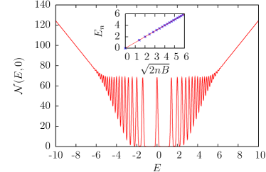
Figure 1: Local density of states (arbitrary units) as a function of energy for the Hamiltonian (2) in the absence of a potential $V({\bf x})$ but in the presence of a magnetic field $B=B_{0}$. The energy is measured in units of $E_{0}=\hbar v_{F}/x_{0}$. The inset shows the energy $E$ as a function of the Landau level index $n$ (counting starts at $E=0$).

The accuracy of the method is demonstrated in Fig. 1, where we show the local density of states in the presence of a magnetic field ($B=B_{0}$) but in the absence of the potential $V({\bf x})$. At low energies one observes a sequence of Landau levels at positions $E_{n}=\pm E_{0}\sqrt{2nB/B_{0}}$ as expected from the analytical calculations. The spectrum is reproduced with a very high accuracy as it is shown in the inset of Fig. 1. Due to the truncation of the Chebyshev expansion the Landau levels in our figure have a finite width. As a consequence only a few discrete peaks are seen in the low energy region of the density of states, whereas at larger energy the Landau levels overlap such that one observes the linear density of states of the Dirac Hamiltonian.

Figure 2: Local density of states in the presence of a Gaussian potential with $V_{0}=-2E_{0}$ and $\sigma=3x_{0}$. The curves correspond to magnetic field strengths $B/B_{0}=0,0.2\dots 2$ (from bottom to top). With the parameters given in the text the energy scale is $E_{0}\approx 33$ meV and the magnetic field scale is $B_{0}\approx 6.6$ T. The potential has a depth of 66 meV and a width of 30 nm.

Figure 2 depicts the local density of states in the presence of a Gaussian potential with $V_{0}=-2E_{0}$ and $\sigma=3x_{0}$. The magnetic field varies from $B=0$ to $B=2B_{0}$ in steps of $\Delta B=0.2B_{0}$. For clarity we use offsets for the different magnetic field strengths. With $x_{0}=10$ nm and $v_{F}=5\times 10^{5}$ m/s the energy and magnetic field scales are $E_{0}\approx 33$ meV and $B_{0}\approx 6.6$ T. With our choice of parameters we are close to the values given in Refs. [Cheng et al., 2010] and [Hanaguri et al., 2010]. For zero magnetic field (lowest curve), the potential shifts the minimum of the density of states to a lower energy, and the density of states is no longer symmetric around the minimum. In the presence of a magnetic field one observes several Landau levels. However, the negative branch of the Landau levels is suppressed. Only for large magnetic field peaks that correspond to negative Landau level index $n$ reappear.

In order to obtain a qualitative understanding of these findings we present now a semiclassical analysis of the effect. We start with the classical equations of motion for wave packets formed by the eigenstates of the Hamiltonian (2),

$${\bf v} = \pm v_{F}{\hat{\bf k}}$$ (6)

$$\hbar\dot{\bf k} = -e\,{\bf v}\times{\bf B}-\nabla V({\bf x});$$ (7)

here ${\bf v}$ is the velocity, ${\hat{\bf k}}$ is the direction of ${\bf k}$ and the plus and minus sign correspond to particles and holes respectively. In the absence of the potential $V({\bf x})$ the magnetic force constrains the trajectories to circles with cyclotron radius $r_{c}=\hbar k/eB$. Using the Bohr-Sommerfeld quantization condition

$$I=\oint{\bf p}\cdot d{\bf x}=2\pi\hbar(n+\gamma),\quad{\bf p}=\hbar{\bf k}-e{\bf A}$$ (8)

with $\gamma=0$ the correct Landau level spectrum is recovered. Generally, $\gamma$ is the sum of a Berry phase and a Maslov contribution which cancel each other in the case of massless Dirac fermions, see for example Ref. [Fuchs et al., 2010] for a recent discussion.

In the presence of the electrostatic potential $V({\bf x})$ there is a competition between magnetic and electric forces. Considering for example a circular motion around the origin we find a modified cyclotron radius,

$$r_{c}=\frac{\hbar v_{F}k}{ev_{F}B\pm V^{\prime}(r_{c})}.$$ (9)

For a Gaussian potential with negative $V_{0}$ the derivative $V^{\prime}(r_{c})$ is positive and thus the potential reduces the cyclotron radius for electrons (due to the extra force directing towards the center of the cyclotron orbit) but enlarges the cyclotron radius for holes. An analogous behavior is found for the action integral $I$: for a given $k$, the potential increases the action of closed loops for holes and decreases the action for the electrons.

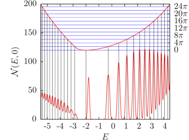
Figure 3: Semiclassical analysis of the Landau levels for $B=B_{0}$ in the presence of a potential $V({\bf x})$. The upper curve shows the action $I/\hbar$ for closed trajectories starting and ending ${\bf x}=0$ (right axis), the lower curve shows the local density of states ${\cal N}(E,{\bf x}\!=\!0)$ (left axis). The depth and width of the potential $V({\bf x})$ are the same as in Fig. 2.

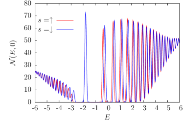
Figure 4: Spin resolved density of states ${\cal N}_{s}(E,{\bf x}\!=\!0)$ for the same parameters as in Fig. 3.

The upper part of Fig. 3 depicts numerical results for the action $I$ (divided by $\hbar$) for trajectories that start and end at ${\bf x}=0$ as a function of energy. The trajectories are closed, in general they are not periodic but form rosette-like orbits. Clearly for electrons $(E>V_{0}=-2E_{0})$ the action grows much slower as a function of energy than for the holes just as we argued before for circular trajectories. In the lower part of Fig. 3 we show again the local density of states at ${\bf x}=0$, but compared to Fig. 2 we increased the number of Chebyshev polynomials such that the peaks become sharper. Due to this improved resolution the density of states below $E\approx-2E_{0}$ is no longer smooth but also shows a pronounced peak structure. Furthermore, with exception of the two peaks at $E\approx-2E_{0}$ and $E\approx-3E_{0}$, the Bohr-Sommerfeld quantization condition accurately reproduces the peak positions.

Figure 4 shows the spin resolved density of states for the parameters of Fig. 3. The central peak is fully spin-polarized which is not a surprise since already in the absence of $V({\bf x})$ the $n=0$ Landau level is spin-polarized. More surprisingly the electrostatic potential $V({\bf x})$ splits the higher Landau levels into two spin polarized peaks, an effect for which we do not have a semiclassical explanation at the moment.

In summary we investigated the Landau levels in the surface states of a topological insulator. In order to mimic the influence of an STM tip on the local density of states we included an electrostatic potential in the description. For a realistic set of parameters the local density of states behaves very similar to what has been observed experimentally, namely the negative branch of Landau levels appears to be suppressed. The origin of the effect is the widening of the cyclotron orbits of the holes due to the electric force. We notice that similar STM studies exist also for the Landau levels in graphene, where the low energy physics is governed by Dirac cones as well. In a study of graphene on graphite, where metallic graphite can screen the electrostatic effects due to the STM tip, both branches of Landau levels have been observed Li et al. (2009). On the other hand in graphene on insulating SiO₂ substrates there is no such screening and only one branch of Landau levels is observed experimentallyLuican et al. (2011), similar to what was found for Bi₂Se₃. This suggests that in both cases the electrostatic field due to the STM tip is the origin of the asymmetric STM spectra.

We thank the Deutsche Forschungsgemeinschaft (SPP1285) for financial support.

References

- Moore (2009) J. E. Moore, Nat. Phys. 5, 378 (2009).
- Hasan and Kane (2010) M. Hasan and C. Kane, Rev. Mod. Phys. 82, 3045 (2010).
- Konig et al. (2007) M. Konig, S. Wiedmann, C. Brune, A. Roth, H. Buhmann, L. W. Molenkamp, and S.-C. Qi, X.-Land Zhang, Science 318, 766 (2007).
- Hsieh et al. (2008) D. Hsieh, D. Qian, L. Wray, Y. Xia, Y. S. Hor, R. J. Cava, and M. Z. Hasan, Nature 452, 970 (2008).
- Hsieh et al. (2009a) D. Hsieh, Y. Xia, L. Wray, D. Qian, A. Pal, J. H. Dil, F. Meier, J. Osterwalder, C. L. Kane, G. Bihlmayer, et al., Science 323, 919 (2009a).
- Hsieh et al. (2009b) D. Hsieh, Y. Xia, D. Qian, L. Wray, J. H. Dill, F. Meier, J. Osterwalder, L. Patthey, J. G. Checkelsky, N. P. Ong, et al., Nature 460, 1101 (2009b).
- Chen et al. (2009) Y. L. Chen, J. G. Analytis, J.-H. Chu, Z. K. Liu, S.-K. Mo, X. L. Qi, H. J. Zhang, D. H. Lu, X. Dai, Z. Fang, et al., Science 325, 178 (2009).
- Xia et al. (2009) Y. Xia, D. Qian, D. Hsieh, L. Wray, A. Pal, H. Lin, A. Bansil, D. Grauer, Y. S. Hor, R. J. Cava, et al., Nature Physics 5, 398 (2009).
- Kuroda et al. (2010) K. Kuroda, M. Arita, K. Miyamoto, M. Ye, J. Jang, A. Kimura, E. E. Krasovskii, E. V. Chulkov, H. Iwasawa, T. Okuda, et al., Phys. Rev. Lett. 105, 076802 (2010).
- Kane and Mele (2005a) C. L. Kane and E. J. Mele, Phys. Rev. Lett. 95, 226801 (2005a).
- Kane and Mele (2005b) C. L. Kane and E. J. Mele, Phys. Rev. Lett. 95, 146802 (2005b).
- Bernevig et al. (2006) B. A. Bernevig, T. L. Hughes, and S.-C. Zhang, Science 313, 1757 (2006).
- Moore and Balents (2007) J. E. Moore and L. Balents, Phys. Rev. B 75, 121306 (2007).
- Fu et al. (2007) L. Fu, C. L. Kane, and E. J. Mele, Phys. Rev. Lett. 98, 106803 (2007).
- Murakami (2007) S. Murakami, New Journal of Physics 9, 356 (2007).
- Roy (2009) R. Roy, Phys. Rev. B 79, 195322 (2009).
- Cheng et al. (2010) P. Cheng, C. Song, T. Zhang, Y. Zhang, Y. Wang, J.-F. Jia, J. Wang, Y. Wang, B.-Z. Zhu, X. Chen, et al., Phys. Rev. Lett. 105, 076801 (2010).
- Hanaguri et al. (2010) T. Hanaguri, K. Igarashi, M. Kawamura, H. Takagi, and T. Sasagawa, Phys. Rev. B 82, 081305 (2010).
- Zhang et al. (2010) Y. Zhang, K. He, C. Chang, C.-L. Song, L.-L. Wang, X. Chen, J.-F. Jia, Z. Fang, X. Dai, W.-Y. Shan, et al., Nature Physics 6, 584 (2010).
- Zhang et al. (2009) H. Zhang, C.-X. Liu, X.-L. Qui, X. Dai, Z. Fang, and S.-C. Zhang, Nature Physics 5, 483 (2009).
- Fu (2010) L. Fu, Phys. Rev. Lett. 103, 266801 (2010).
- Chen (2011) X. Chen (2011), private communication.
- Weisse et al. (2006) A. Weisse, G. Wellein, A. Alvermann, and H. Fehske, Rev. Mod. Phys. 78, 275 (2006).
- Fuchs et al. (2010) J. N. Fuchs, F. Piechon, M. O. Goerbig, and G. Montambaux, Eur. Phys. J. B 77, 351 (2010).
- Li et al. (2009) G. Li, A. Luican, and E. Y. Andrei, Phys. Rev. Lett. 102, 176804 (2009).
- Luican et al. (2011) A. Luican, G. Li, and E. Y. Andrei, Phys. Rev. B 83, 041405(R) (2011).